Invariant Extended Kalman Filtering Using Two Position Receivers for Extended Pose Estimation

Consider the matrix Lie group $\mathcal{G}$ composed of $n\times n$ invertible matrices with $m$ degrees of freedom that is closed under matrix multiplication [15]. The matrix Lie algebra associated with $\mathcal{G}$ is denoted $\mathfrak{g}$. An element of $\mathfrak{g}$ can be mapped to $\mathcal{G}$ using the exponential map, $\exp(\cdot):\mathfrak{g}\rightarrow\mathcal{G}$. Similarly, an element of $\mathcal{G}$ can be mapped to $\mathfrak{g}$ using the matrix natural logarithm, $\log(\cdot):\mathcal{G}\rightarrow\mathfrak{g}$. The linear operator $(\cdot)^{\wedge}$ maps $\mathbb{R}^{m}\to\mathfrak{g}$, and $(\cdot)^{\vee}$ maps $\mathfrak{g}\to\mathbb{R}^{m}$. When $\delta{\boldsymbol{\xi}}\in\mathbb{R}^{m}$ is small, $\mathrm{exp}\left(\delta{\boldsymbol{\xi}}^{\wedge}\right)$ can be approximated as $\mathrm{exp}\left(\delta{\boldsymbol{\xi}}^{\wedge}\right)\approx\mbf{1}+\delta{\boldsymbol{\xi}}^{\wedge}$.

The IEKF framework has four conditions that must be met for it to be used. First, the measurement model must be either left or right invariant. The second and third conditions are that the invariant error and invariant innovation must be consistent with the left or right invariance of the measurement model. Fourth, the process model must be group affine. In this section, each of these components will be discussed, with a focus on left invariance.

Given the left-invariant measurement model Definition II.1, error given by Definition II.2, innovation from Definition II.3, and a process model that satisfies Definition II.4, the IEKF framework can be used [9].

Consider a process model of the form

$\displaystyle{\dot{\mbf{X}}}(t)$

$\displaystyle=\mbf{F}(\mbf{X}(t),\mbf{u}(t))+\mbf{X}(t)\mbf{W}(t),$

(5)

where $\mbf{F}(\mbf{X}(t),\mbf{u}(t))$ is group affine, $\mbf{X}(t)\in\mathcal{G}$, $\mbf{u}(t)\in\mathbb{R}^{n_{u}}$ is the process input, and $\mbf{W}(t)=\mbf{w}(t)^{\wedge}\in\mathfrak{g}$ is zero-mean Gaussian white process noise. For the remainder of this work, the argument $(t)$ is dropped for conciseness, unless required for clarity. The nonlinear process model can be linearized using the definition of the left-invariant error (2) to yield

$\displaystyle\delta{\dot{\boldsymbol{\xi}}}$

$\displaystyle=\mbf{A}_{\mathrm{c}}\delta{\boldsymbol{\xi}}+\mbf{L}_{\mathrm{c}}\delta\mbf{w},$

(6)

where $\delta\mbf{w}\sim\mathcal{N}(\mbf{0},{\boldsymbol{Q}}\delta(t-\tau))$, and ${\boldsymbol{Q}}$ is the power spectral density. The discrete time prediction is then

	$\displaystyle\check{\mbf{X}}_{k}$	$\displaystyle=\mbf{F}_{k-1}\big({\hat{\mbf{X}}}_{k-1},\mbf{u}_{k-1}\big),$		(7)
	$\displaystyle\check{\mbf{P}}_{k}$	$\displaystyle=\mbf{A}_{k-1}{\hat{\mbf{P}}}_{k-1}\mbf{A}_{k-1}^{\mathsf{T}}+\mbf{L}_{k-1}\mbf{Q}_{k-1}\mbf{L}_{k-1}^{\mathsf{T}},$		(8)

where (7) comes from discretization of (5), and $\mbf{A}_{k-1}$, $\mbf{L}_{k-1}$, and $\mbf{Q}_{k-1}$ come from discretization of (6) and ${\boldsymbol{Q}}$ [16]. The left-invariant innovation can be linearized, again using the definition of the left-invariant error (2), along with the approximation $\delta\mbf{X}_{k}=\exp(\delta{\boldsymbol{\xi}}_{k}^{\wedge})\approx\mbf{1}+\delta{\boldsymbol{\xi}}_{k}^{\wedge}$. In detail,

	$\displaystyle\mbf{z}_{k}$	$\displaystyle=\check{\mbf{X}}_{k}^{-1}(\mbf{X}_{k}\mbf{b}+\mbf{n}_{k}-\check{\mbf{X}}_{k}\mbf{b})=\delta\mbf{X}_{k}^{-1}\mbf{b}-\mbf{b}+\check{\mbf{X}}_{k}^{-1}\mbf{n}_{k}$
		$\displaystyle\approx(\mbf{1}-\delta{\boldsymbol{\xi}}_{k}^{\wedge})\mbf{b}-\mbf{b}+\check{\mbf{X}}_{k}^{-1}\delta\mbf{n}_{k}=\mbf{H}_{k}\delta{\boldsymbol{\xi}}_{k}+\mbf{M}_{k}\delta\mbf{n}_{k}.$		(9)

where $\mbf{M}_{k}=\check{\mbf{X}}_{k}^{-1}$ and $\delta\mbf{n}_{k}\sim\mathcal{N}\left(\mbf{0},\mbf{R}_{k}\right)$. The state correction is then

$\displaystyle{\hat{\mbf{X}}}_{k}=\check{\mbf{X}}_{k}\exp\Big(-(\mbf{K}_{k}\mbf{z}_{k})^{\wedge}\Big),$

(10)

which is consistent with the definition of the left-invariant error in (2). The Kalman gain is

$\displaystyle\mbf{K}_{k}=\check{\mbf{P}}_{k}\mbf{H}_{k}^{\mathsf{T}}\mbf{S}_{k}^{-1},$

(11)

where

$\displaystyle\mbf{S}_{k}=\mbf{H}_{k}\check{\mbf{P}}_{k}\mbf{H}_{k}^{\mathsf{T}}+\mbf{M}_{k}\mbf{R}_{k}\mbf{M}_{k}^{\mathsf{T}}.$

(12)

The normalized innovation squared (NIS) is defined as [17, 18]

$\displaystyle\epsilon_{z,k}=\mbf{z}_{k}^{\mathsf{T}}\mbf{S}_{k}^{-1}\mbf{z}_{k},$

(13)

where $\mbf{S}_{k}$ is given in (12). The NIS is $\chi^{2}$ distributed of degree $n_{z}$. The average NIS,

$\displaystyle\bar{\epsilon}_{z,k}=\frac{1}{N}\sum_{i=1}^{N}\epsilon^{i}_{z,k},$

(14)

is also $\chi^{2}$ distributed of degree $Nn_{z}$, and can therefore be compared to the critical $\chi^{2}$ values to verify the consistency of the estimator [17]. Dividing the result of (14) by $n_{z}$ results in a values close to one for consistent systems [19]. A value greater than one indicates an optimistic estimator, where the errors to covariance ratio is too large, or the estimates include significant bias [17]. A value less than one indicates that the estimator is pessimistic.

The following notation is used throughout this work. A physical vector $\underrightarrow{p}$ resolved in $\mathcal{F}_{a}$ is denoted $\mbf{p}_{a}$, and resolved in $\mathcal{F}_{b}$ is denoted as $\mbf{p}_{b}$. The relationship between $\mbf{p}_{a}$ and $\mbf{p}_{b}$ is $\mbf{p}_{a}=\mbf{C}_{ab}\mbf{p}_{b}$, or $\mbf{p}_{b}=\mbf{C}_{ba}\mbf{p}_{a}$, where $\mbf{C}_{ab}=\mbf{C}_{ba}^{\mathsf{T}}=\mbf{C}_{ba}^{-1}\in SO(3)$ is the direction cosine matrix (DCM). The cross product of two physical vectors resolved in a frame, such as $\mathcal{F}_{b}$, is denoted $\mbf{p}_{b}^{\times}\mbf{q}_{b}=-\mbf{q}_{b}^{\times}\mbf{p}_{b}$.

Consider a rigid body, with body frame $\mathcal{F}_{b}$, an inertial frame $\mathcal{F}_{a}$, and a datum point $w$. An IMU with an accelerometer and a rate gyro is mounted at point $z_{0}$ on the rigid body. Two position receivers, which could be GPS or UWB receivers, are placed at points $z_{1}$ and $z_{2}$, respectively, on the rigid body. The physical vector describing $z_{0}$ relative to $w$ is $\underrightarrow{r}^{z_{0}w}$, and the physical vector describing $z_{1}$ relative to $z_{2}$ is denoted $\underrightarrow{r}^{z_{1}z_{2}}$. The velocity of point $z_{0}$ relative to point $w$ relative to $\mathcal{F}_{a}$ is $\underrightarrow{v}^{z_{0}w/a}$.

The two-receiver extended pose estimation problem to be solved is, given an accelerometer, a rate gyro, and two position receivers, estimate the position, velocity, and attitude as described by $\mbf{r}_{a}^{z_{0}w}$, $\mbf{v}_{a}^{z_{0}w/a}$, and $\mbf{C}_{ab}$, respectively. This problem follows a loosely-coupled GPS-INS formulation [17].

The rate gyro, $\mbf{u}^{1}_{b}$, and accelerometer, $\mbf{u}_{b}^{2}$, measurement models are

	$\displaystyle\mbf{u}^{1}_{b}$	$\displaystyle={\boldsymbol{\omega}}_{b}^{ba}-\mbf{w}^{1}_{b},$		(15)
	$\displaystyle\mbf{u}_{b}^{2}$	$\displaystyle=\mbf{C}_{ab}^{\mathsf{T}}({\dot{\mbf{v}}}_{a}^{z_{0}w/a}-\mbf{g}_{a})-\mbf{w}_{b}^{2},$		(16)

where ${\boldsymbol{\omega}}_{b}^{ba}$ is the angular velocity of $\mathcal{F}_{b}$ relative to $\mathcal{F}_{a}$ resolved in $\mathcal{F}_{b}$, ${\dot{\mbf{v}}}_{a}^{z_{0}w/a}$ is the acceleration of point $z_{0}$ relative to point $w$ with respect to $\mathcal{F}_{a}$ resolved in $\mathcal{F}_{a}$, $\mbf{g}_{a}$ is the gravity vector resolved in $\mathcal{F}_{a}$, and both $\mbf{w}_{b}^{1}\sim\mathcal{N}(0,{\boldsymbol{Q}}^{\omega}(t)\mathcal{\delta}(t-\tau))$ and $\mbf{w}_{b}^{2}\sim\mathcal{N}(0,{\boldsymbol{Q}}^{\mathrm{a}}(t)\mathcal{\delta}(t-\tau))$ are zero-mean Gaussian white measurement noise. Using (15) and (16) the continuous-time kinematic equations defining the time evolution of the rigid body are

	$\displaystyle{\dot{\mbf{C}}}_{ab}$	$\displaystyle=\mbf{C}_{ab}(\mbf{u}_{b}^{1}+\mbf{w}_{b}^{1})^{\times},$		(17)
	$\displaystyle{\dot{\mbf{v}}}_{a}^{z_{0}w/a}$	$\displaystyle=\mbf{C}_{ab}(\mbf{u}_{b}^{2}+\mbf{w}_{b}^{2})+\mbf{g}_{a},$		(18)
	$\displaystyle{\dot{\mbf{r}}}^{z_{0}w}_{a}$	$\displaystyle=\mbf{v}_{a}^{z_{0}w/a}.$		(19)

Biases are not included in (15) and (16), nor (17), (18), (19), because it is assumed that the sensor data has been calibrated such that biases are negligible, which is the case in the experiments presented in Section IV-B. Biases can be included in the “imperfect” IEKF framework [20, 21].

Position measurements from two position receivers affixed to the rigid body are available. Each position measurement is of the form

$\displaystyle\mbf{y}_{k}^{\textrm{pos},i}$

$\displaystyle=\mbf{r}^{z_{i}w}_{a_{k}}+\mbf{n}_{k}^{\textrm{pos},i},\;\;\;i=1,2,$

(20)

where $\mbf{n}_{k}^{i}\sim\mathcal{N}(\mbf{0},\mbf{R}^{z_{i}w})$. Subtracting the two position measurements yields a relative position measurement,

$\displaystyle\mbf{y}_{k}^{\textrm{rel}}$

$\displaystyle=\mbf{y}_{k}^{\textrm{pos},2}-\mbf{y}_{k}^{\textrm{pos},1}=\mbf{r}^{z_{2}w}_{a_{k}}-\mbf{r}^{z_{1}w}_{a_{k}}+\mbf{n}_{k}^{\textrm{rel}},$

(21)

where $\mbf{n}_{k}^{\textrm{rel}}=\mbf{n}_{k}^{\textrm{pos},2}-\mbf{n}_{k}^{\textrm{pos},1}$. Notice that $\mbf{y}_{k}^{\textrm{rel}}$ in (21) can be written

$\displaystyle\mbf{y}_{k}^{\textrm{rel}}$

$\displaystyle=\mbf{C}_{ab_{k}}\mbf{r}^{z_{2}z_{1}}_{b}+\mbf{n}_{k}^{\textrm{rel}},$

(22)

where $\mbf{r}^{z_{2}z_{1}}_{b}$ is the known distance, the baseline, between the two receivers in $\mathcal{F}_{b}$. Some sensor suites, such as a moving baseline real-time kinematic (RTK) GPS system, will provide both (20) and (22) directly [22].

The kinematic equations (17), (18), (19) can collectively be written using the group of double direct isometries, $SE_{2}(3)$ [9, 20], to form the IEKF process model. In particular,

$\displaystyle{\dot{\mbf{X}}}=\mbf{F}(\mbf{X},\mbf{u}_{b})+\mbf{X}\mbf{W}_{b}$

(23)

where $\mbf{u}_{b}=[\mbf{u}_{b}^{1^{\mathsf{T}}}\;\;\;\mbf{u}_{b}^{2^{\mathsf{T}}}\;\;\;\mbf{0}]^{\mathsf{T}}$, $\mbf{W}_{b}^{\vee}=\mbf{w}_{b}=[\mbf{w}_{b}^{1^{\mathsf{T}}}\;\;\;\mbf{w}_{b}^{2^{\mathsf{T}}}\;\;\;\mbf{0}]^{\mathsf{T}}$,

	$\displaystyle\mbf{X}$	$\displaystyle=\left[\begin{array}[]{ ccc}\mbf{C}_{ab}&\mbf{v}_{a}^{z_{0}w/a}&\mbf{r}_{a}^{z_{0}w}\\ \mbf{0}&1&0\\ \mbf{0}&0&1\end{array}\right]\in SE_{2}(3),$
	$\displaystyle\mbf{W}_{b}=\mbf{w}_{b}^{\wedge}$	$\displaystyle=\left[\begin{array}[]{ ccc}\mbf{w}_{b}^{1^{\times}}&\mbf{w}_{b}^{2}&\mbf{0}\\ \mbf{0}&0&0\\ \mbf{0}&0&0\end{array}\right]\in\mathfrak{se}_{2}(3),$
	$\displaystyle\mbf{F}(\mbf{X},\mbf{u}_{b})$	$\displaystyle=\left[\begin{array}[]{ ccc}\mbf{C}_{ab}\mbf{u}_{b}^{1^{\times}}&\mbf{C}_{ab}\mbf{u}_{b}^{2}+\mbf{g}_{a}&\mbf{v}_{a}^{z_{0}w/a}\\ \mbf{0}&1&0\\ \mbf{0}&0&1\end{array}\right].$

The function (III-D) is group affine [9]. The subblocks composing the left-invariant error (2) between $\mbf{X}\in SE_{2}(3)$ and ${\hat{\mbf{X}}}\in SE_{2}(3)$ are

	$\displaystyle\delta\mbf{C}_{ab}$	$\displaystyle=\mbf{C}_{ab}^{\mathsf{T}}{\hat{\mbf{C}}}_{ab},$		(33)
	$\displaystyle\delta\mbf{v}^{z_{0}w/a}_{a}$	$\displaystyle=\mbf{C}_{ab}^{\mathsf{T}}({\hat{\mbf{v}}}^{z_{0}w/a}_{a}-\mbf{v}^{z_{0}w/a}_{a}),$		(34)
	$\displaystyle\delta\mbf{r}^{z_{0}w}_{a}$	$\displaystyle=\mbf{C}_{ab}^{\mathsf{T}}({\hat{\mbf{r}}}^{z_{0}w}_{a}-\mbf{r}^{z_{0}w}_{a}).$		(35)

These error definitions are used to linearize the process model, resulting in a linearized model of the form (6) where

$\displaystyle\delta{\boldsymbol{\xi}}=\left[\begin{array}[]{ ccc}\delta{\boldsymbol{\xi}}^{\theta^{\mathsf{T}}}&\delta{\boldsymbol{\xi}}^{v^{\mathsf{T}}}&\delta{\boldsymbol{\xi}}^{r^{\mathsf{T}}}\end{array}\right]^{\mathsf{T}},$

and the Jacobians $\mbf{A}_{\mathrm{c}}$ and $\mbf{L}_{\mathrm{c}}$ are [20]

	$\displaystyle\mbf{A}_{\mathrm{c}}$	$\displaystyle=\left[\begin{array}[]{ ccc}-{\mbf{u}_{b}^{1}}^{\times}&\mbf{0}&\mbf{0}\\ -{\mbf{u}_{b}^{2}}^{\times}&-{\mbf{u}_{b}^{1}}^{\times}&\mbf{0}\\ \mbf{0}&\mbf{1}&-{\mbf{u}_{b}^{1}}^{\times}\\ \end{array}\right],$
	$\displaystyle\mbf{L}_{\mathrm{c}}$	$\displaystyle=\left[\begin{array}[]{ ccc}-\mbf{1}&\mbf{0}&\mbf{0}\\ \mbf{0}&-\mbf{1}&\mbf{0}\\ \mbf{0}&\mbf{0}&\mbf{0}\\ \end{array}\right].$

The Jacobian $\mbf{A}_{\mathrm{c}}$ in (III-D) is independent of the state estimate. This is an attribute of group affine systems, a key ingredient in the IEKF framework. Additionally, $\mbf{L}_{\mathrm{c}}$ in (III-D) happens to be constant and independent of the state estimate as well, although the IEKF framework does not guarantee this. The state-estimate independence of $\mbf{A}_{\mathrm{c}}$ and $\mbf{L}_{\mathrm{c}}$, that does not hold for the MEKF presented in Appendix-A, is an advantage of the IEKF that often results in better filter performance, in particular in the transient phase [9]. The continuous-time linearized process model is discretized using the method described in [16, 23].

The measurement model is composed of $\mbf{y}_{k}^{\textrm{pos},1}$, as defined in (20), and the relative position of two position receivers, as given in (21). Using (20) and (21), the measurement model is

$\displaystyle\mbf{y}_{k}=\left[\begin{array}[]{ c}\mbf{y}_{k}^{1}\\ \mbf{y}_{k}^{2}\end{array}\right],$

where

	$\displaystyle\mbf{y}_{k}^{1}$	$\displaystyle=\left[\begin{array}[]{ c}\mbf{y}_{k}^{\textrm{pos},1}\\ 0\\ 1\end{array}\right]=\mbf{X}_{k}\left[\begin{array}[]{ c}\mbf{r}_{b}^{z_{1}z_{0}}\\ 0\\ 1\end{array}\right]+\left[\begin{array}[]{ c}\mbf{n}_{k}^{\textrm{pos},1}\\ 0\\ 0\end{array}\right],$
	$\displaystyle\mbf{y}_{k}^{2}$	$\displaystyle=\left[\begin{array}[]{ c}\mbf{y}_{k}^{\textrm{rel}}\\ 0\\ 0\end{array}\right]=\mbf{X}_{k}\left[\begin{array}[]{ c}\mbf{r}_{b}^{z_{2}z_{1}}\\ 0\\ 0\end{array}\right]+\left[\begin{array}[]{ c}\mbf{n}_{k}^{\textrm{rel}}\\ 0\\ 0\end{array}\right].$

Both (III-D) and (III-D) composing (III-D) are left-invariant measurement models of form given in (1). The left-invariant innovation is then

$\displaystyle\mbf{z}_{k}$

$\displaystyle=\left[\begin{array}[]{ c}\mbf{z}^{1}_{k}\\ \mbf{z}^{2}_{k}\end{array}\right]=\left[\begin{array}[]{ cc}\check{\mbf{X}}_{k}^{-1}&\mbf{0}\\ \mbf{0}&\check{\mbf{X}}_{k}^{-1}\end{array}\right]\left[\begin{array}[]{ c}\mbf{y}^{1}_{k}-{\hat{\mbf{y}}}^{1}_{k}\\ \mbf{y}^{2}_{k}-{\hat{\mbf{y}}}^{2}_{k}\end{array}\right].$

The linearization of both $\mbf{z}^{i}_{k}$, $i=1,2$ in (III-D) is accomplished using the definition of the left-invariant error (2) and the approximation $\delta\mbf{X}_{k}=\exp(\delta{\boldsymbol{\xi}}_{k}^{\wedge})\approx\mbf{1}+\delta{\boldsymbol{\xi}}_{k}^{\wedge}$, as detailed in (9). The Jacobians in (9) specific to (III-D) are

$\displaystyle\mbf{H}_{k}$

$\displaystyle=\left[\begin{array}[]{ ccc}(\mbf{r}_{b}^{z_{1}z_{0}})^{\times}&\mbf{0}&-\mbf{1}\\ (\mbf{r}_{b}^{z_{2}z_{1}})^{\times}&\mbf{0}&\mbf{0}\\ \end{array}\right],\;\;\;\mbf{M}_{k}=\left[\begin{array}[]{ cc}\check{\mbf{C}}_{{ab}_{k}}^{-1}&\mbf{0}\\ \mbf{0}&\check{\mbf{C}}_{{ab}_{k}}^{-1}\end{array}\right],$

where redundant rows of zeros have been removed on both the left and right-hand sides of (9). The Jacobian $\mbf{H}_{k}$ is independent of the state-estimate, as is guaranteed by the IEKF formulation, while Jacobian $\mbf{M}_{k}$ is not state-estimate independent.

100 Monte Carlo trials were run on the same 50 second trajectory. Each Monte Carlo trial introduces sensor noise, randomly sampled with the covariances from $\mbf{Q}_{\mathrm{d}}=\mathrm{diag}\Big(\mbf{Q}_{\mathrm{d}}^{\theta},\mbf{Q}_{\mathrm{d}}^{a}\Big)$, with $\mbf{Q}_{\mathrm{d}}^{\theta}=0.0012^{2}\times\mbf{1}\;(\mathrm{rad})^{2}$ and $\mbf{Q}_{\mathrm{d}}^{a}=0.0025^{2}\times\mbf{1}\;(\mathrm{m/s^{2}})^{2}$. The initial positions and velocities are randomly sampled from ${\hat{\mbf{P}}}_{0}=\mathrm{blkdiag}\Big((\pi/3)^{2}\times\mbf{1}\;(\mathrm{rad})^{2},0.1^{2}\times\mbf{1}\;(\mathrm{m/s})^{2},0.1^{2}\times\mbf{1}\;(\mathrm{m})^{2}\Big)$. In order to highlight the advantage of the IEKF in the transient phase, a constant initial error of $\pi/3$ (rad) is introduced into each of the components of the attitude. The prediction step is performed at a frequency of 250 Hz, while the correction step is executed at 15 Hz. The RMSE in attitude, position and velocity for each Monte Carlo run was computed and reported in Fig. 1. The bars represent the average RMSE, while the upper and lower error bounds represent the 2.5 and 97.5 percentile, respectively, meaning that 95% of trials lie between these bounds.

Fig. 1 shows that the two-receiver IEKF outperforms the two-receiver MEKF and single-receiver IEKF in its estimates of all states. These results are consistent with the literature, since the advantage of state-independent Jacobians emanates when the state estimates are highly erroneous, as is the case when the initial error is large. Thus, the steady state performance of the two-receiver IEKF and two-receiver MEKF should be similar, while the transient performance of the two-receiver IEKF should show improvement over the two-receiver MEKF [11]. Fig. 1 shows that the improvement in attitude is small, while the greater advantage arises in position and velocity estimates. The advantage arising from the two-receiver IEKF framework appears in the comparison of RMSE in velocity, where the single-receiver IEKF has lower RMSE than the two-receiver MEKF.

The former results do not give any indication of the consistency of the filters. For this, the average NIS test was used. The comparison is presented in Fig. 2. All filters were found to become consistent within less than 5 seconds, with the initial inconsistency caused by the error introduced in the attitude initialization.

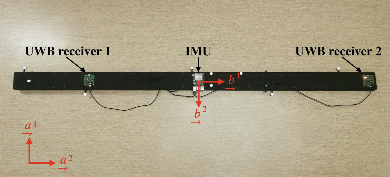
The proposed approach was further validated through an experiment. An IMU and two UWB receivers were mounted on a rigid body, shown in Fig. 3, with the two UWB receivers placed 1.80 m apart. Five UWB anchors were placed at various heights around a room where the experiments were conducted. Trials of approximately two minutes were recorded, during which the rigid body was moved around a volume measuring 5 m $\times$ 4 m $\times$ 2 m. A motion capture system was used to record ground truth measurements. The accelerometer and gyroscope measurements were collected at a frequency of 250 Hz, while the UWB position measurements arrived at a frequency of about 17 Hz.

The process noise power spectral density (PSD) matrices were computed using the Allan variance method, generated using static IMU data, according to [24]. The measurement noise covariance matrix was computed through comparison of the recorded measurements and motion capture ground truth measurements. The resulting PSD and covariance matrices are

	$\displaystyle{\boldsymbol{Q}}(t)$	$\displaystyle=\mathrm{diag}\Big({\boldsymbol{Q}}^{\omega}(t),{\boldsymbol{Q}}^{\mathrm{a}}(t)\Big),$		(73)
	$\displaystyle{\boldsymbol{Q}}^{\omega}(t)$	$\displaystyle=\mathrm{diag}\Big(2.0^{2},2.0^{2},1.8^{2}\Big)\times 10^{-4}\;(\mathrm{rad})^{2},$		(74)
	$\displaystyle{\boldsymbol{Q}}^{\mathrm{a}}(t)$	$\displaystyle=\mathrm{diag}\Big(1.7^{2},1.5^{2},2.4^{2}\Big)\times 10^{-2}\;(\mathrm{m/s^{2}})^{2},$		(75)
	$\displaystyle\mbf{R}$	$\displaystyle=\mathrm{diag}\Big(\mbf{R}^{z_{1}w},\mbf{R}^{z_{2}w}\Big),$		(76)
	$\displaystyle\mbf{R}^{z_{1}w}$	$\displaystyle=\mathrm{diag}\Big(1.3^{2},1.1^{2},1.9^{2}\Big)\times 10^{-2}\;(\mathrm{m})^{2},$		(77)
	$\displaystyle\mbf{R}^{z_{2}w}$	$\displaystyle=\mathrm{diag}\Big(1.9^{2},1.6^{2},2.6^{2}\Big)\times 10^{-2}\;(\mathrm{m})^{2}.$		(78)

As in simulation, the attitude was initialized with an error of $\pi/3$ (rad) to demonstrate the advantage of the IEKF in situations in which there is large uncertainty on the initial attitude. The RMSE for each of the filters is presented in Fig. 4. It should be noted that ground truth velocity was not measured directly, but rather computed using the ground truth positions. This process introduces some error into the ground truth velocity, which is used to compute the error in the velocity estimates.

The filter performance on experiment data emulates the simulation performance. The two-receiver IEKF attitude estimate improves greatly over the single-receiver IEKF, but show only slight improvement over the two-receiver MEKF. This improvement arises in the transient phase where the effect of having state-dependent Jacobians impacts the MEKF but not the IEKF. The two-receiver IEKF and MEKF perform equivalently at steady state, which is consistent with previous literature. It should be noted that a transient phase does not only occur during initialization, but can also occur if a sensor is unavailable (that is, “drops out”) for an extended period of time.

The distance between receivers was studied experimentally using the platform shown in Fig. 3. The receiver placement was decreased between experimental runs. For each of the experiment runs, the three filters were compared using RMSE as a performance metric. The resulting RMSEs of each filter are shown in Fig. 5. While reporting the single-receiver IEKF performance as a function of receiver spacing may seem imprecise, the receiver spacing is used to categorize the various experiment runs. While the RMSE of the single-receiver should be consistent across runs, certain inconsistencies arise from factors such as the manual trajectory generation and hardware flaws during data collection. Thus, the single-receiver RMSE are computed and reported for each run. The same data is presented in terms of percent differences between each filter and the two-receiver IEKF in Fig. 6.

The two-receiver IEKF has the greatest advantage over the single-receiver IEKF in attitude estimates, in which a maximum improvement of 110%, and a minimum improvement of 23% was observed. With greater receiver spacing, the advantage introduced by the addition of a second receiver becomes increasingly evident in the position and attitude estimates. Even with the receivers spaced 0.1 m apart, the addition of a second receiver enhances the attitude estimates by 23%, and the position estimates by 2%. Over all spacings, the two-receiver IEKF performance improved attitude estimates by 71% over the single-receiver IEKF and by 7% over the two-receiver MEKF. The position estimates were improved by 19% over the single-receiver IEKF and 4% over the two-receiver MEKF.

While the focus of this work is on the use of the IEKF, the invariant measurement, invariant error, invariant innovation, and group-affine process model can be used within an invariant UKF (IUKF) framework [25]. Simulation results comparing the performance of the two-receiver IUKF, the two-receiver multiplicative UKF (MUKF), and the single-receiver IUKF are presented in Fig. 7, without a derivation of the filter equations. The derivation of the filters equations follows that of [25].

The average RMSE in attitude of the IUKF is slightly lower than that of the UKF, but the IUKF has slightly larger upper and lower percentile bounds than the UKF. The IUKF definitively outperforms the MUKF in terms of position and velocity RMSE. Also, given the same parameters, the three UKF variants, with results presented in Fig. 7, outperform the corresponding EKF variant, with results presented in Fig. 1. Therefore, should adequate computing resources be available such that a UKF variant can be used, and performance beyond what the two-receiver versions of the MEKF, MUKF, and IEKF can provide is required, the IUKF is attractive.

References

- [1] A. Barrau and S. Bonnabel “A Mathematical Framework for IMU Error Propagation with Applications to Preintegration” In IEEE International Conference on Robotics and Automation, 2020, pp. 5732–5738
- [2] Clark. Cohen “Attitude Determination” In Global Positioning System: Theory and App. 2 Reston, VA: AIAA, 1996, pp. 519–538
- [3] Rui Hirokawa and Takuji Ebinuma “A low-cost tightly coupled GPS/INS for small UAVs augmented with multiple GPS antennas” In Navigation 56.1, 2009, pp. 35–44
- [4] Peter Buist, P. Teunissen, Gabriele Giorgi and Sandra Verhagen “Multiplatform Instantaneous GNSS Ambiguity Resolution for Triple- and Quadruple-Antenna Configurations with Constraints” In International Journal of Navigation and Observation 2009, 2009
- [5] G.I. Emel’yantsev, B.A. Blazhnov and A.P. Stepanov “Specific Features of Constructing a Dual-Mode GNSS Gyrocompass as a Tightly-Coupled Integrated System” In Gyroscopy and Navigation 9, 2018, pp. 97–105
- [6] Eun-Hwan Shin “Estimation techniques for low-cost inertial navigation”, 2005
- [7] Jong-Hwa Yoon and Huei Peng “A Cost-Effective Sideslip Estimation Method Using Velocity Measurements From Two GPS Receivers” In IEEE Transactions on Vehicular Technology 63.6, 2013, pp. 2589 –2599
- [8] Yushi Hao, Aigong Xu, Xin Sui and Yulei Wang “A Modified Extended Kalman Filter for a Two-Antenna GPS/INS Vehicular Navigation System” In Sensors 18, 2018, pp. 3809
- [9] Axel Barrau and Silvère Bonnabel “The Invariant Extended Kalman Filter as a Stable Observer” In IEEE Transactions on Automatic Control 62.4, 2017
- [10] Simo Särkkä “Bayesian Filtering and Smoothing” Cambridge University Press, 2013
- [11] Axel Barrau and Silvere Bonnabel “Three examples of the stability properties of the invariant extended Kalman filter” In IFAC-PapersOnLine 50.1, 2017, pp. 431–437
- [12] Jonathan Arsenault “Practical Considerations and Extensions of the Invariant Extended Kalman Filtering Framework”, 2019
- [13] Paul Richardson, Weidong Xiang and Dan Shan “An outdoor UWB tracking system to improve safety of semi-autonomous vehicle operations” In International Journal of Ultra Wideband Communications and Systems 1, 2010
- [14] Tobias Nageli, Benjamin Hepp and Otmar Hilliges “Omni-directional person tracking on a flying robot using occlusion-robust ultra-wideband signals” In International Conference on Intelligent Robots and Systems, 2016, pp. 189–194
- [15] Brian Hall “Lie Groups, Lie Algebras, and Representations” Springer, 2014
- [16] C Van “Computing integrals involving the matrix exponential” In IEEE Transactions on Automatic Control 23.3, 1978, pp. 424–440
- [17] Yaakov Bar-Shalom, X Li and Kirubarajan Thiagalingam “Estimation with Applications to Tracking and Navigation” Wiley, 2001
- [18] Zhaozhong Chen, Christoffer Heckman, Simon Julier and Ahmed Nisar “Weak in the NEES?: Auto-tuning Kalman Filters with Bayesian Optimization” In Fusion, 2018
- [19] Axel Barrau and Silvère Bonnabel “An EKF-SLAM algorithm with consistency properties”, 2015 arXiv:1510.06263
- [20] Axel Barrau “Non-linear state error based extended Kalman filters with applications to navigation”, 2015
- [21] S. Heo and C.. Park “Consistent EKF-Based Visual-Inertial Odometry on Matrix Lie Group” In IEEE Sensors Journal 18.9, 2018, pp. 3780–3788
- [22] Rachel Schmalzried “The Role of RTK in the Autonomous System Sensor Suite” Swift Navigation, 2017
- [23] Jay Farrell “Aided Navigation” McGraw-Hill, 2008
- [24] Oliver Woodman “An Introduction to Inertial Navigation” University of Cambridge, Tech. Report 696, 2007
- [25] Martin Brossard, Silvère Bonnabel and Jean-Philippe Condomines “Unscented Kalman filtering on Lie groups” In International Conference on Intelligent Robots and Systems, 2017, pp. 2485–2491