ALMA Observations of NGC 604 in M33: Physical Properties of Molecular Clouds2020ALMA Observations of NGC 604 in M33: Physical Properties of Molecular Clouds–7
Abstract
We present Atacama Large Millimeter/submillimeter Array (ALMA) observations of line and 104 GHz continuum emission from NGC 604, a giant H II region (GHR) in the nearby spiral galaxy M33. Our high spatial resolution images (, corresponding to pc physical scale) allow us to detect fifteen molecular clouds. We find spatial offsets between the and 104 GHz continuum emission and also detect continuum emission near the centre of the GHR. The identified molecular clouds have sizes ranging from 5-21 pc, linewidths of 0.3-3.0 and luminosity-derived masses of . These molecular clouds are in near virial equilibrium, with a spearman correlation coefficient of 0.98. The linewidth-size relationship for these clouds is offset from the corresponding relations for the Milky Way and for NGC 300, although this may be an artefact of the dendrogram process.
Keywords:
galaxies: individual (M33) –ISM: clouds – ISM: individual objects (NGC 604)–radio lines:ISM1 Introduction
Star formation occurs within cold, dense Giant Molecular Clouds (GMCs) embedded within the interstellar medium (ISM). GMCs show turbulent internal motions and are predominantly comprised of molecular hydrogen. Observations of GMCs within our own Galaxy have shown they have spatial scales of up to a hundred parsec, large scale velocity dispersions which are supersonic, and masses up to solar masses (Heyer & Dame 2015). Three key empirical GMC scaling relations, which have become officially accepted diagnostics for the physical conditions and structure, were first identified by Larson 1981. Later studies by other authors (e.g., (Solomon et al. 1987; Rice et al. 2016, and references therein)) have demonstrated the ubiquity of these scaling relations, commonly called Larson’s relations, for Milky Way clouds. The first scaling relation is the size - linewidth relation, where the velocity line width of giant molecular clouds is proportional to the 0.5 power of the size, . The second relation deals with GMC’s virial equilibrium, where gravitational potential energy and kinetic energy are in approximate equilibrium (Larson 1981; Solomon et al. 1987; Heyer et al. 2009; Heyer & Dame 2015). This equilibrium manifests as a direct correlation between the masses estimated from related methods, e.g. the virial mass () and the luminous mass (e.g, from in our case). A final implication of the Larson scaling relationships is that the surface density of molecular is approximately constant (e.g.,). This proceeds from the Third Law which showed that where R is an estimate of its physical size of the cloud and is its mass volume density (Larson 1981). This clear universality in cloud structure was verified in other Galactic studies (Solomon et al. 1987; Heyer et al. 2009). Some extragalactic studies have also found correlations between GMC size and mass (Bolatto et al. 2008; Hughes et al. 2010). However, Faesi et al. 2018 notes that these extragalactic observations have low sensitivities, with the majority of pixels in GMCs near the sensitivity threshold, so the correlations may or may not be physically meaningful.
In as much as Milky Way GMCs have been the foundation of GMC studies, observations of these sources are affected by a number of challenging phenomena, mainly the blending of emission from multiple clouds along the line of sight. External galaxies offer an opportunity to study GMCs and star formation in different environments, including different metallicities and different galaxy types, and to make comparisons with our own Galaxy. With the emergence of modern (sub)millimeter interferometers and large single-dish telescopes, it has become possible to resolve individual GMCs in nearby galaxies (Schruba et al. 2017).
GMCs are traced by emission from the low rotational (J) states of the CO molecules, which are excited via collisions at temperatures ranging from (van Dishoeck & Black 1988). A number of high resolution CO observations have been done in external galaxies, including M33 (Engargiola et al. 2003; Rosolowsky et al. 2003; Rosolowsky et al. 2007; Gratier et al. 2012) and NGC 300 (Faesi et al. 2018). More recently, the Physics at High Angular resolution in Nearby GalaxieS project has mapped CO(2-1) emission from multiple galaxies, resolving the molecular gas reservoir into individual GMCs across the full disc (Schinnerer et al. 2019).
M33 is a flocculent spiral galaxy in the Local Group. It is metal poor but gas rich and has a metallicity of (Rosolowsky & Simon 2008). It is at a distance of (Freedman et al. 1991; Kam et al. 2015) and an inclination of (Kam et al. 2015), which allows us to resolve gas components with minimum contamination along the line of sight and to map their inner structure of GMCs. Earlier studies of GMCs in this galaxy include those by Wilson et al. 1997; Rosolowsky et al. 2007; Tosaki et al. 2007; Miura et al. 2010; Gratier et al. 2010; Gratier et al. 2012; Tabatabaei et al. 2014.
The giant H II region (GHR) NGC 604 is located in the northern arm of M33. This region has attracted interest because it has the highest star formation rate in the entire galaxy (Miura et al. 2012). The GHR has been observed in radio emission (Viallefond et al. 1992; Wilson & Scoville 1992; Churchwell & Goss 1999; Tosaki et al. 2007; Miura et al. 2010), optical emission (Drissen et al. 1993) and X-ray emission (Tüllmann et al. 2008). Based on these previous studies, the H nebula has a core-halo structure extending out to . It contains more than 200 O-type stars that are surrounded by photoionized filaments and shells (Relaño & Kennicutt 2009).
Faesi et al. 2018 notes that determining true physical signatures in extragalactic studies is made difficult due to the wide range of source finding techniques and deferring observational characteristics (angular, spectral, and sensitivity) used. Hence, new analysis techniques are needed to overcome these problems and to understand the universality of Larson’s relations.
In this work, we present a dendrogram analysis of ALMA observations of 13CO(J=1-0) and 104 GHz continuum emission from NGC 604. These observations have better resolutions and sensitivities compared to prior observations, which helps to overcome many of the issues highlighted by Faesi et al. 2018. We look at whether the 13CO emission from NGC 604 obey Larson’s relations in the same way as the 12CO emission from the same region as presented by Wilson & Scoville 1992. Using these new data, we measure the properties of the clouds and examine the state of the star formation in the region, and we compare to results presented earlier by Miura et al. 2010. We present the observations and data reduction process in Section 2, the structure decomposition analysis and measurements of the cloud properties in Section 3, and the results in Section 4. We discuss our results in Section 5 and summarize our results in Section 6.
2 Observations and Data Reduction
We use archival ALMA Band 3 observations of the 13CO(J=1-0) (110.27 GHz) line emission from NGC 604 obtained during Cycle 2 (project code 2013.1.00639.S; PI: T. Tosaki). The target was observed with the ALMA 12m array on 18 January 2015 for a total of 60 minutes on-source. ALMA was in configuration C34-2/1 with 34 antennas (although two are flagged as unusable) arranged with baselines ranging from 15 m to 349 m, which yields a minimum beam angular resolution of 2.2 arcsec and a maximum recoverable scale of 29 arcsec (at 110.27 GHz). This corresponds to physical scales of 9 to 116 pc at the distance of to M33. The observed field of view is 43 arcsec. J2258-2758 was used as a bandpass calibrator, Mars as a flux calibrator and J0237+2848 as a phase calibrator.
Four spectral windows were used in the observations. Three of the spectral windows cover the 13CO (J=1-0) at 110.2 GHz, C18CO(J=1-0) at 109.8 GHz and CH3OH at 96.7 GHz lines; each of these spectral windows contained 180 channels with widths of 244.14 kHz, covering a bandwidth of 117.2 MHz. The fourth spectral window covered continuum emission from 98.56 - 99.50 GHz using 3840 channels with widths of 244.14 kHz (). Only the 13CO (J=1-0) and continuum emission are detected in this data.
The Common Astronomy Software Application package (McMullin et al. 2007, CASA; ) version 5.6.1 was used to process the data. We first performed the standard pipeline calibration on the visibility data and then produced line cubes and continuum images using tclean. We set the pixel scale for both the continuum and line images to 0.36 arcsec. The channel width for the 13CO image was set to 0.664 km s-1. We used Briggs weighting with the robust parameter set to 0.5 to improve the angular resolution of the final images without severely compromising the image sensitivity. The synthesized beam sizes are 3.2 2.4 arcsec for the line data and 3.9 2.8 arcsec for the continuum data. The achieved rms sensitivity in the line data is 2.6 mJy beam-1 and continuum is 0.04 mJy beam-1. The calibration uncertainty is expected to be 5% (Braatz et al. 2020).
The 13CO(J=1-0) integrated intensity map and the 104 GHz continuum map are shown in Figure 1. As an additional visualization aid, the 13CO(J=1-0) emission is overlaid as contours on the continuum image in Figure 2.


The 104 GHz continuum emission detected in NGC 604 (as shown in the bottom right panel of Figure 1) is believed to be dominated by free-free emission (as indicated by the spectral energy distribution analyses of other galaxies by Peel et al. 2011, Bendo et al. 2015, and Bendo et al. 2016) that originates from OB stars within NGC 604. We find spatial offsets between 13CO line and 104 GHz continuum emission as shown in Figure 2. See Section 5 for more details on their distribution.
3 Structure Decomposition and Cloud Properties
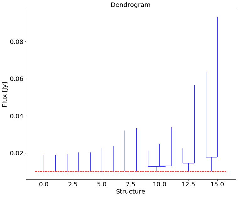

To identify structures within the 13CO(J=1-0) image cube, we used the astrodendro package, which decomposes emission into a hierarchy of nested structures (Rosolowsky et al. 2008; Colombo et al. 2015). This dendrogram technique, provide a precise representation of the topology of star forming complexes. Parameters were chosen so that the algorithm could identify local maxima in the cube above the 4 level that were also 3 above the merge level with adjacent structures. Isorsurfaces surrounding the local maxima were categorized as trunks, branches or leaves based on whether they were the largest contiguous structures (trunks), intermediate in scale (branches) or had no resolved substructure (leaves). The resulting dendrogram for 13CO(J=1-0) in NGC 604 is shown in Figure 3. We identified 20 structures in the entire dendrogram, consisting of 15 leaves and 4 branches, using the above parameters. Spectra for the peak brightness pixels, for each leaf, are presented in Appendix 7. We use letter L to represent the leaf number in our labels for the structures. From now onwards, we shall refer to these leaves as molecular clouds.
We compared our results with the results from Miura et al. 2010, who show observations of 12CO(J=1-0) line emission from NGC 604 as observed by the Nobeyama Millimeter Array. We detected and resolved the clouds that they labelled NMA 4, 7, 8, 9, 10. We, however, are not able to detect NMA 1, 3, 6, 11 and 12 above our 4 noise level. This is because Miura et al. 2012 used a lower detection threshold of 3. If we lower our detection threshold to 3, we can detect these sources, but we also detect additional spurious noise in the maps. Given this situation, we chose to use only sources detected at the higher threshold. NMA 2 and 5 are outside of our field of view. We proceed to determine the basic properties of the identified structures at this point.
The basic properties of the identified structures are also determined by astrodendro using the bijection approach (Rosolowsky et al. 2008). We extracted the molecular cloud properties using the approach described by Wong et al. 2017. These properties include spatial and velocity centroids (), the integrated flux F, the rms line-width (defined as the intensity-weighted second moment of the structure along the velocity axis), the position angle of the major axis , and the scaling terms along the major and minor axes, and . From these basic quantities, we calculated additional cloud properties; these are listed in Table 1. The rms spatial size is given by the geometric mean of and . The spherical radius is set to 1.91 following Solomon et al. 1987 and Rosolowsky & Leroy 2006. The luminosity-based mass for 13CO(J=1-0) is computed using
| (1) |
from Rosolowsky et al. 2008, where is the assumed conversion factor. This calculation includes a factor of 1.36 to account for the mass of helium. Changes to the first term or conversion factor are represented with the parameter . We have adopted based on the average conversion factor of for nearby disc spiral galaxies found by Cormier et al. 2018. This average is equivalent to what would be expected for the conversion factor for a galaxy with . This is close to the abundance of measured for NGC 604 (Esteban et al. 2009). The scatter in value is 0.3 dex (Cormier et al. 2018). This uncertainty means that masses will have a systematic error of about a factor of 2.
The virial mass of molecular clouds derived assuming virial equilibrium is
| (2) |
where is the linewidth in and R is the spherical radius in pc. This formulation assumes a truncated power-law density distribution of with and with the assumption that magnetic fields and external pressure are negligible (Solomon et al. 1987). In this equation, is only defined for finite clouds with resolved radii.
The average molecular gas surface density is defined as
| (3) |
where is the luminosity-based mass.
The dynamic state of a cloud is described by the the virial parameter which is given by
| (4) |
Allowing for uncertainties in measured parameters, a virtual ratio of is generally taken to mean that a cloud is gravitational bound. However, a cloud with an ratio significantly lower than this would need additional internal support (e.g. magnetic fields) to survive for longer than the usual dynamical timescale (Faesi et al. 2018).
The uncertainties in the molecular clouds properties R, , and are computed using a bootstrap method with 50 iterations. The bootstrapping determines errors by generating several trial clouds from the original cloud data. The properties are measured for each trial cloud, and the uncertainties are estimated from the variance of properties derived from these resampled and remeasured datasets. The final uncertainty in each property is the standard deviation of the bootstrapped values scaled by the square root of the oversampling rate. The bootsrap method is described in detail by Rosolowsky & Leroy 2006 and Rosolowsky et al. 2008. Other uncertainties in derived properties presented in this work are calculated using the standard propagation of errors.
4 Results
| MC ID | RA | DEC | ||||||||
|---|---|---|---|---|---|---|---|---|---|---|
| J2000 | J2000 | (pc) | ||||||||
| L1 | +30:46:57.07 | -245.7 | ||||||||
| L2 | +30:46:59.84 | -249.1 | ||||||||
| L3 | +30:47:01.85 | -243.8 | ||||||||
| L4 | +30:46:57.98 | -244.4 | ||||||||
| L5 | +30:46:48.88 | -243.1 | ||||||||
| L6 | +30:46:41.92 | -241.1 | ||||||||
| L7 | +30:46:37.09 | -252.0 | ||||||||
| L8 | +30:46:31.80 | -247.1 | ||||||||
| L9 | +30:46:30.44 | -252.4 | ||||||||
| L10 | +30:46:25.48 | -219.2 | ||||||||
| L11 | +30:46:21.91 | -220.5 | ||||||||
| L12 | +30:46:14.66 | -217.9 | ||||||||
| L13 | +30:46:46.12 | -223.2 | ||||||||
| L14 | +30:46:57.35 | -229.8 | ||||||||
| L15 | +30:46:58.45 | -226.5 |
The properties of the the fifteen molecular clouds (leaves) identified by our dendrogram analysis are presented in Table 1, and the left panel of Figure 4 shows the the locations of these clouds. The two right panels in Figure 4 show magnified versions of the NMA-8 region. Miura et al. 2010 only detected a single object in this region, but we detected four separate sources and resolved the structure in the brightest source. We discuss this more in Section 5.
4.1 Scaling Relations
Figure 5 shows the size-linewidth relation for our sources. The clouds in blue are the fifteen clouds identified as unresolved substructure (leaves) by our analysis technique, and those in red are the branches which harbor resolved substructures. To investigate whether our molecular clouds are in virial equilibrium, we plotted molecular mass versus virial mass in Figure 6. In the absence of other forces, the virial parameter, which is the ratio of kinetic to gravitational potential energies, indicates the level of boundedness. The unbound ones are those with , while the bound are those with between 1-2, and the ones with are in a state of forming stars.

4.1.1 Size - Line width Relation
The size-linewidth relation is commonly known as Larson’s first law. The relates the line-width in to the radius in parsecs (Wong et al. 2017). Large CO linewidths seen at parsec scales are evidence that these clouds are turbulent. It then follows from the size-linewidth relationship that there is a turbulent cascade of energy through the ISM (Faesi et al. 2018) and that the form of this turbulence is described by its power law slope (1/2 for compressible, 1/3 for incompressible, (McKee & Ostriker 2007)).
Figure 5 shows the size-linewidth relation for our GMCs. We see that there is a clear trend, with larger clouds having larger linewidths, as is found in Milky Way clouds. The Spearman correlation coefficient for these data has the value of , which indicates that there is a correlation between size and linewidths of GMCs in NGC 604. We also show in Figure 5 the Milky Way power-law slope (green solid line) from Solomon et al. 1987 and the extragalactic slope (green dashed line) from Faesi et al. 2018 for NGC 300. The relation for the NGC 604 clouds does not match the Milky Way and NGC 300 slopes; the linewidths at small radii for the NGC 604 data fall below the Milky Way and NGC 300 relations. In the figure, we plot results done by Wilson & Scoville 1992 (black points). Despite their results having considerable poor resolution, () compared to our ALMA ). There is consistency between the two results on large sizes having large linewidths (WS92 results) and smaller sizes having smaller linewidths (our clouds). The features are a typical characteristics of a turbulent spectrum which has a range of scales with increasing kinetic energy at large scales. We find their results to be in agreement with both the Milky Way and NGC 300 relations. Wong et al. 2017 and Wong et al. 2019 found a similar offset in the size-linewidth relationship between Milky Way and Large Magellanic Cloud data. They ascribed the discrepancy to two factors. The first was the limitations in resolution of the Large Magellanic Cloud observations. The second was the bijection approach in dendrogram analysis. The rms linewidths in the dendrogram analysis tend to be underestimated for structures which are defined by high isocontour levels such as leaves because the full width of the spectral line is truncated by the isosurface boundary (Rosolowsky 2005; Rosolowsky et al. 2008). NGC 604 and 30 Dor, one of the region Wong et al. 2017 studied, are both sites of massive star formation surrounding giant H II regions and would both be places with high isocontour levels, so both of these locations could plausibly be affected by this truncation bias. It is worth noting that other extragalactic studies have found no strong correlation between size and linewidth (Colombo et al. 2014; Maeda et al. 2020).
4.1.2 Molecular Mass - Virial Mass Relations
The Milky Way observations have shown that the majority of GMCs are in self-gravitational equilibrium (Larson 1981; Solomon et al. 1987; Heyer et al. 2009; Heyer & Dame 2015, e.g.,). This leads to a direct correlation between and the mass measured through other independent method (in our case the 13CO luminosity). Recent extragalactic studies of NGC 300 by Faesi et al. 2018 and NGC 1300 by Maeda et al. 2020 have found a strong correlation between and and a low scatter in near unity. We show in Figure 6 that the clouds in NGC 604 are in near virial equilibrium and that the data are strongly correlated, with a Spearman coefficient of . Most of the clouds are lying below a one-to-one relation, illustrating that the masses estimated from the luminosities are slightly higher than the virial masses, which is a direct consequence of underestimating linewidths as discussed in the previous section. These clouds have virial parameters ranging from 0.2-1.1, indicating that some clouds are in virial equilibrium while others could be in a state of forming stars. The Wilson & Scoville 1992 data, which are also shown in Figure 6, largely seem consistent with the results from NGC 604.

5 Discussion
As seen in Figure 2, both continuum and 13CO(J=1-0) emission are detected near the centre of the H II region, although at locations further from the centre of the H II region, we found a few locations with only 13CO(J=1-0) emission. The regions which are associated with continuum emission are actively forming stars. We have labelled the three continuum sources with the abbreviation MMS (millimetre source), with MMS1 corresponding to L5, MMS2 corresponding to L4, and MMS4 corresponding to L1 as seen in the bottom right panel of Figure 1. Muraoka et al. 2020 also identified three sources in this region. Our MMS2 corresponds to their MMS2, but they were able to resolve the brighter source, which we labelled as MMS1, into two sources labelled MMS1 and MMS3 (which is why we labelled our third source as MMS4).
Regions only detected in 13CO(J=1-0) emission are dense molecular clouds with no active star formation. In these regions, atomic hydrogen (HI) could be forming H2, and these clouds may form stars as the H II expands. Previous studies in this region have found similar results and suggested that GMCs in NGC 604 are at different evolutionary stages, which would lead to sequential star formation induced by the expansion of GHR (Tosaki et al. 2007; Miura et al. 2010). To make comparison to the work done previously by Miura et al. 2010, we use the nomenclature for their clouds and identify how many clouds we have resolved in each major GMC.
5.1 NMA-8
We have resolved NMA-8, the largest GMC in NGC 604 found by (Miura et al. 2010), into four individual molecular clouds that we labelled L3, L4, L5 and L6. It is possible that L5 contains two or more smaller clouds, but we could not separate them into smaller clouds when applying astrodendro to the 13CO data. Based on the 12CO(J=1-0) observations, NMA-8 is known to be the most massive () GMC in the GHR (Miura et al. 2010, and references therein). Using 13CO(J=1-0), we estimate a virial mass of and a molecular mass of in NMA-8, which is a factor of 5 less than the 12CO(J=1-0) molecular mass presented by Miura et al. 2010. This is attributed to 13CO(J=1-0) only tracing the dense gas, hence, resolving away diffuse gas which make up large scale structure and also to the underestimation of linewidths. Our computed 13CO molecular mass for NMA-8 is comparable to the Orion A GMC, which has an estimated 12CO molecular mass of (Wilson et al. 2005). The NMA-8 molecular mass estimate from 13CO is higher than the virial mass estimated from the linewidths and the spherical radius but agree within the errors. The estimated molecular mass of in L5 is comparable to Orion B in the Milky Way, which has a mass of (Wilson et al. 2005).
The association of L4 and L5 with 104 GHz continuum sources, which is expected to be dominated by free-free emission (Peel et al. 2011; Bendo et al. 2015; Bendo et al. 2016, e.g. ), clearly indicates that they are undergoing star formation. However, the peaks in the 13CO emission from these sources do no coincide exactly with the continuum peaks, as seen in the right zoomed panel of Figure 4. The continuum peaks lie closer to the centre of the H II region than the 13CO peaks. This misalignment in this region has been reported previously by Miura et al. 2010. The spatial offset between these peaks is an indication that these two tracers do trace different regions. The center has photoionizing stars which photoionize the gas surrounding which we trace by continuum in turn. The 13CO(1-0) line, being the lowest J-transition with a very low excitation temperature, preferentially traces cold dense molecular gas away from the centre. It is thus insensitive to the warm gas traced by the continuum emission. Earlier studies in NGC 604 by Muraoka et al. 2012 also found a temperature gradient in the NGC 604 clouds.
5.2 Other GMCs in NGC 604
We have for the first time resolved NMA-7 into three sources (L10, L11, and L12) and NMA-9 into three sources (L7, L8, and L9). Other than L1, these other GMCs are not associated with continuum sources and are not associated with ongoing star formation. NMA-9 is the second massive and second largest complex in the imaged area, with a molecular mass of about . As we indicated before, the clouds without continuum emission could be places where the atomic gas is currently forming molecular gas, but when the GHR expands, these clouds may form stars.
Generally, NGC 604 molecular clouds indicates that they are at different evolutionary stages within the H II region, with some being associated with both continuum and line emission while others only line emission. Additional dendrogram analyses with higher resolution data will be necessary to explore these phenomena in more detail.
6 Conclusions
We have presented ALMA 13CO(1-0) and 104 GHz continuum observations of NGC 604. Using the astrodendro algorithm, we identified 15 molecular clouds. The main results are given as follows:
- 1.
The identified molecular clouds have sizes ranging from 5-21 pc, linewidths , of 0.3-3.0 and luminosity-derived masses , of . These sizes, linewidths and masses are comparable to typical Milky Way molecular clouds.
- 2.
For the first time, this work has resolved NMA-8, the most massive GMC, into four molecular clouds named L3, L4, L5 and L6, with L5 showing two clear peaks. We detect 104 GHz continuum emission from L5, although it is offset from the 13CO emission.
- 3.
We only detect 104 GHz continuum emission near the centre of GHR. Further out of the centre, only 13CO line emission is detected. This indicates that the GMCs in NGC 604 are in different evolutionary stages as previously suggested by Tosaki et al. 2007 and Miura et al. 2010. Additionally, we find a spatial misalignment between 13CO and 104 GHz continuum in NGC 604. The center has photoionizing stars which photoionize the gas surrounding which we trace by continuum in turn while the 13CO(1-0) line, being the lowest J-transition with a very low excitation temperature, preferentially traces cold dense molecular gas away from the centre. It is thus insensitive to the warm gas traced by the continuum emission. This is a confirmation of what previous studies found in the same region.
- 4.
We have found that the sizes and linewidths are correlated for the NGC 604 GMCs but that the relationship is offset from the Milky Way scaling relation. This may be a consequence of the limited resolution of our data or artefact of the dendrogram analysis as applied to bright sources. The relation for the clouds in NGC 604 is consistent with the idea of compressible hierarchical turbulence in the ISM within this region.
- 5.
We find a clear one-to-one relationship between virial mass and luminous mass indicating that the clouds in NGC 604 are in virial equilibrium. This relation is consistent with the earlier relation published by WS92.
- 6.
The virial parameter ranges from 0.2-1.1. This result entails that some of the molecular clouds are below which means that not only are they in a state of forming stars but photoionizing stars have been formed. Other clouds have values near unity, which means that they are in virial equilibrium.
Acknowledgements
We thank the anonymous referee for the helpful comments in improving this manuscript. Research reported in this publication was supported by a Newton Fund project, DARA (Development in Africa with Radio Astronomy), and awarded by the UK’s Science and Technology Facilities Council (STFC) - grant reference ST/R001103/1. This work makes use of the following ALMA data: ADS/JAO.ALMA2013.1.00639.S. ALMA is a partnership of ESO (representing its member states), NSF (USA) and NINS (Japan), together with NRC (Canada), MOST and ASIAA (Taiwan), and KASI (Republic of Korea), in cooperation with the Republic of Chile. The Joint ALMA Observatory is operated by ESO, AUI/NRAO and NAOJ. This research made use of astrodendro, a Python package to compute dendrograms of Astronomical data 11
1
http://www.dendrograms.org/. This research made use of astropy,22
2
http://www.astropy.org a community-developed core Python package for Astronomy (Astropy
Collaboration et al. 2013; Astropy
Collaboration et al. 2018).
DATA AVAILABILITY: The raw data underlying this article is available on the ALMA archive: ADS/JAO.ALMA2013.1.00639.S. The calibrated image data generated for this research will be shared on reasonable request to the corresponding author.
References
- Astropy Collaboration et al. (2013) Astropy Collaboration et al., 2013, A&A, 558, A33
- Astropy Collaboration et al. (2018) Astropy Collaboration et al., 2018, AJ, 156, 123
- Bendo et al. (2015) Bendo G. J., Beswick R. J., D’Cruze M. J., Dickinson C., Fuller G. A., Muxlow T. W. B., 2015, MNRAS, 450, L80
- Bendo et al. (2016) Bendo G. J., Henkel C., D’Cruze M. J., Dickinson C., Fuller G. A., Karim A., 2016, MNRAS, 463, 252
- Bolatto et al. (2008) Bolatto A. D., Leroy A. K., Rosolowsky E., Walter F., Blitz L., 2008, ApJ, 686, 948
- Braatz et al. (2020) Braatz J., Impellizzeri V., Biggs A., P. S., 2020, ALMA Cycle 8 Proposer’s Guide, version 1.0. Joint ALMA Observatory, Santiago
- Churchwell & Goss (1999) Churchwell E., Goss W. M., 1999, ApJ, 514, 188
- Colombo et al. (2014) Colombo D., et al., 2014, ApJ, 784, 3
- Colombo et al. (2015) Colombo D., Rosolowsky E., Ginsburg A., Duarte-Cabral A., Hughes A., 2015, MNRAS, 454, 2067
- Cormier et al. (2018) Cormier D., et al., 2018, MNRAS, 475, 3909
- Drissen et al. (1993) Drissen L., Moffat A. F. J., Shara M. M., 1993, in Cassinelli J. P., Churchwell E. B., eds, Astronomical Society of the Pacific Conference Series Vol. 35, Massive Stars: Their Lives in the Interstellar Medium. p. 528
- Engargiola et al. (2003) Engargiola G., Plambeck R. L., Rosolowsky E., Blitz L., 2003, ApJS, 149, 343
- Esteban et al. (2009) Esteban C., Bresolin F., Peimbert M., García-Rojas J., Peimbert A., Mesa-Delgado A., 2009, ApJ, 700, 654
- Faesi et al. (2018) Faesi C. M., Lada C. J., Forbrich J., 2018, ApJ, 857, 19
- Freedman et al. (1991) Freedman W. L., Wilson C. D., Madore B. F., 1991, ApJ, 372, 455
- Gratier et al. (2010) Gratier P., et al., 2010, A&A, 522, A3
- Gratier et al. (2012) Gratier P., et al., 2012, A&A, 542, A108
- Heyer & Dame (2015) Heyer M., Dame T. M., 2015, ARA&A, 53, 583
- Heyer et al. (2009) Heyer M., Krawczyk C., Duval J., Jackson J. M., 2009, ApJ, 699, 1092
- Hughes et al. (2010) Hughes A., et al., 2010, MNRAS, 406, 2065
- Kam et al. (2015) Kam Z. S., Carignan C., Chemin L., Amram P., Epinat B., 2015, MNRAS, 449, 4048
- Larson (1981) Larson R. B., 1981, MNRAS, 194, 809
- Maeda et al. (2020) Maeda F., Ohta K., Fujimoto Y., Habe A., 2020, MNRAS,
- McKee & Ostriker (2007) McKee C. F., Ostriker E. C., 2007, ARA&A, 45, 565
- McMullin et al. (2007) McMullin J. P., Waters B., Schiebel D., Young W., Golap K., 2007, in Shaw R. A., Hill F., Bell D. J., eds, Astronomical Society of the Pacific Conference Series Vol. 376, Astronomical Data Analysis Software and Systems XVI. p. 127
- Miura et al. (2010) Miura R., et al., 2010, ApJ, 724, 1120
- Miura et al. (2012) Miura R. E., et al., 2012, ApJ, 761, 37
- Muraoka et al. (2012) Muraoka K., Tosaki T., Miura R., Onodera S., Kuno N., Nakanishi K., Kaneko H., Komugi S., 2012, PASJ, 64, 3
- Muraoka et al. (2020) Muraoka K., et al., 2020, ApJ, 903, 94
- Peel et al. (2011) Peel M. W., Dickinson C., Davies R. D., Clements D. L., Beswick R. J., 2011, MNRAS, 416, L99
- Relaño & Kennicutt (2009) Relaño M., Kennicutt Robert C. J., 2009, ApJ, 699, 1125
- Rice et al. (2016) Rice T. S., Goodman A. A., Bergin E. A., Beaumont C., Dame T. M., 2016, ApJ, 822, 52
- Rosolowsky (2005) Rosolowsky E., 2005, PASP, 117, 1403
- Rosolowsky & Leroy (2006) Rosolowsky E., Leroy A., 2006, PASP, 118, 590
- Rosolowsky & Simon (2008) Rosolowsky E., Simon J. D., 2008, ApJ, 675, 1213
- Rosolowsky et al. (2003) Rosolowsky E., Engargiola G., Plambeck R., Blitz L., 2003, ApJ, 599, 258
- Rosolowsky et al. (2007) Rosolowsky E., Keto E., Matsushita S., Willner S. P., 2007, ApJ, 661, 830
- Rosolowsky et al. (2008) Rosolowsky E. W., Pineda J. E., Kauffmann J., Goodman A. A., 2008, ApJ, 679, 1338
- Schinnerer et al. (2019) Schinnerer E., et al., 2019, ApJ, 887, 49
- Schruba et al. (2017) Schruba A., et al., 2017, ApJ, 835, 278
- Solomon et al. (1987) Solomon P. M., Rivolo A. R., Barrett J., Yahil A., 1987, ApJ, 319, 730
- Tabatabaei et al. (2014) Tabatabaei F. S., et al., 2014, A&A, 561, A95
- Tosaki et al. (2007) Tosaki T., Miura R., Sawada T., Kuno N., Nakanishi K., Kohno K., Okumura S. K., Kawabe R., 2007, ApJ, 664, L27
- Tüllmann et al. (2008) Tüllmann R., et al., 2008, ApJ, 685, 919
- Viallefond et al. (1992) Viallefond F., Boulanger F., Cox P., Lequeux J., Perault M., Vogel S. N., 1992, A&A, 265, 437
- Wilson & Scoville (1992) Wilson C. D., Scoville N., 1992, ApJ, 385, 512
- Wilson et al. (1997) Wilson C. D., Walker C. E., Thornley M. D., 1997, ApJ, 483, 210
- Wilson et al. (2005) Wilson B. A., Dame T. M., Masheder M. R. W., Thaddeus P., 2005, A&A, 430, 523
- Wong et al. (2017) Wong T., et al., 2017, ApJ, 850, 139
- Wong et al. (2019) Wong T., et al., 2019, ApJ, 885, 50
- van Dishoeck & Black (1988) van Dishoeck E. F., Black J. H., 1988, The Photodissociation of Interstellar Co/. p. 168, doi:10.1007/3-540-50438-9_255
Appendix A Peak Spectra for the sources
Presented here in Figure 7 are the spectra (as measured at the peak of the emission) for each of the molecular clouds identified in our dendrogram analysis.


