Integral representation for three-loop banana graph
M.A. Bezuglov1,2,3
1Bogoliubov Laboratory of Theoretical Physics, Joint
Institute for Nuclear Research, Dubna, Russia,
2Moscow Institute of Physics and Technology (State University), Dolgoprudny, Russia,
3Budker Institute of Nuclear Physics, Novosibirsk, Russia,
Abstract
It has recently been shown that two-loop kite-type diagrams can be computed analytically in terms of iterated integrals with algebraic kernels. This result was obtained using a new integral representation for two-loop sunset subgraphs. In this paper, we have developed a similar representation for a three-loop banana integral in dimensions. This answer can be generalized up to any given order in the -expansion and can be calculated numerically both below and above the threshold. We also demonstrate how this result can be used to compute more complex three-loop integrals containing the three-loop banana as a subgraph.
1 Introduction
Computing Feynman diagrams, in particular those with masses is one of the most important problems in modern quantum field theory. There are various methods for calculating these integrals11 1 For a detailed overview of basic methods for computing loop Feynman integrals see [1]., the most effective of which is the differential equations (DE) method[2, 3, 4, 5, 6, 7, 8]. The latter is essentially based on the existence of the so-called integration by parts (IBP) relations [9, 10, 11], due to which any integral from a given family can be represented as a linear combination of a finite number of master integrals. The number of master integrals is fixed and determined by critical points of the integrand in Feynman or Baykov representation[12].
Feynman integrals are usually expressed in terms of special functions. The multiple polylogarithms (MPLs)[13, 14] are proved to be the most successful here. For MPLs there are many functional dependencies and, which is important, they can be calculated numerically with high precision, see [15, 16] and references therein. The system of differential equations for the system of master integral can be solved in terms of MPLs if it can be reduced to the so-called -form[17, 18], which exists only in certain cases. However, it is known that not every system of differential equations can be reduced to the -form. In these cases, MPLs are no longer sufficient. To solve such equations, it is necessary to involve more complex functions, the simplest functions beyond multiple polylogarithms are the so-called elliptic polylogarithms (eMPLs)[19, 20, 21, 22, 23, 24, 25, 26, 27, 28, 29, 30, 31, 32, 33, 34, 35, 36, 37, 38, 39, 40, 41], but wider extensions are also possible[42, 43, 27, 44, 45, 46, 47, 48].
The purpose of this work is to generalize the functions and methods used to calculate the two-loop sunset graph from the work [48] to the case of the three-loop banana graph with equal masses22 2 For other methods of calculating banana integrals, see [39, 44, 27, 49] and references therein, a similar elliptic integral also occurs when calculating the parameter at three loops, see [50, 51, 52] and references therein.. We restrict ourselves to the case in dimensions using the analogy with work [48] where in this case the results were more compact. We also demonstrate with a simple example that the obtained results can be used to compute three-loop diagrams which contain three-loop banana as a subgraph. The remainder of the paper is organized as follows. In section 2, we derive a new representation for three non-trivial master integrals from the three-loop banana family. Next, in section 3, we use this representation to compute a simple three-loop integral containing the three-loop banana as a subgraph. In the last section, we will draw our conclusions. Finally, in the Appendix, we will explain our notations for iterated integrals.
2 Banana graph
First let us define the following notation for the master integrals in the elliptic banana family, see Fig. 1.
| (2.1) |
with and . The vector of four IBP master integrals obtained as a result of IBP reduction[9, 10, 11] can be chosen in the following form:
| (2.2) |
a graphical representation of these master integrals can be found in Fig. 2.
The first master integral is a simple constant and can be expressed analytically in the following form:
| (2.3) |
In order to find the other three master integrals we use Feynman parameter trick for pairing two pairs of propagators 33 3 For an example of using such a trick for non-elliptic cases see [53, 54, 55, 56, 57] and references therein. [58, 59, 60, 48], and we introduce a new family of integrals defined as()
| (2.4) |
where and are Feynman parameters which run through the unit segment(), for the convenience of the reader, we will suppress the dependence on parameters and in the following and we write instead . Then the three nontrivial master integrals from (2.2) can be expressed by integrating the integrals of the family (2.4) over these parameters, we have
| (2.5) |
Now we will use the DE method in order to evaluate the necessary integrals from the family (2.4). The vector of three IBP master integrals can be chosen in such a way that they can be immediately substituted into expression (2.5) without any IBP reduction
| (2.6) |
To evaluate these master integrals we consider their system of differential equations with respect to the variable which is associated with the old variable in the following way
| (2.7) |
where we have introduced new notations
| (2.8) |
With the help of IBP identities the system of differential equations with respect to the variable can be reduced to the -form44 4 The subsequent reduction of system of differential equations to -form was performed with the use of Libra [61] package and the IBP reduction was performed with the help of LiteRed [62, 63] pacadge [17, 18] and we have:
| (2.9) |
where():
| (2.10) |
The particular expressions for coefficient matrices together with transformation matrix to canonical basis () can be found in the accompanying Mathematica notebook. The boundary conditions for (2.9) at () can be found by direct integration, in the Feynman parametrization we have
| (2.11) |
for our values of and , this integral is convergent and can be easily calculated in the form of a Laurent series, the results are as follows:
| (2.12) |
| (2.13) |
| (2.14) |
With the boundary conditions available the solution for all master integrals (2.6) can be found recursively in the regularization parameter , after substituting these results into the formula (2.5) and changing variables from to the results for nontrivial banana master integrals will be as follows:
| (2.15) |
| (2.16) |
and
| (2.17) |
where
| (2.18) |
| (2.19) |
Results for master integrals (2.2) up to corrections can be found in accompanying Mathematica file.
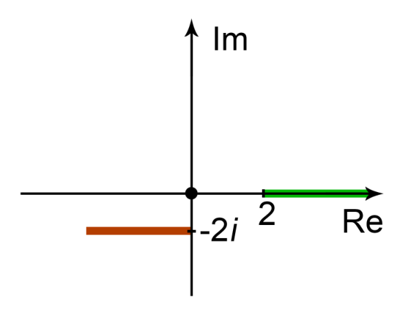
Integrals in equations (2.15),(2.16) and (2.17) as well as higher corrections can be taken numerically, for this it is convenient to change the integration variables and change the contour of integration to , see Fig. 3. The example of numerical integration and their comparison with the sector decomposition method[65, 66, 67, 68, 69, 70, 71] for the corrections and correction for integral can be found in Fig. 7, 7, 7, and 7.
3 Triangle with two massive loops
In the previous section, we obtained an integral representation for the three-loop banana family; in this section, we will show how this representation can be used to compute more complex Feynman integrals. For this purpose, we will use the family associated with the triangle with two massive loops defined as (see Figure 8):
| (3.23) |
with and . The vector of seven IBP master integrals obtained as a result of IBP reduction[9, 10, 11] together with dimension recurrence relations[72] can be chosen in the following form:
| (3.24) |
a graphical representation of these master integrals can be found in Fig. 9.
The first and third master integrals are simple constants and can be written as
| (3.25) |
and
| (3.26) |
where . And the integrals , and were found in the previous section.
To evaluate the remaining master integrals we consider their system of differential equations with respect to . Using balance transformations of [18] via the package [61] the latter can be reduced to the following form:
| (3.27) |
with
| (3.28) |
and
| (3.29) |
| (3.30) |
| (3.31) |
| (3.32) |
And the elements of the canonical basis are related to the elements of the IBP basis (9) as
| (3.33) | ||||
| (3.34) | ||||
| (3.35) | ||||
| (3.36) | ||||
| (3.37) | ||||
| (3.38) | ||||
| (3.39) |
Having obtained the differential system in this form it is easy to see, that the solution for required master integrals and can be obtained recursively in the regularization parameter similarly to what one typically does for differential systems reduced to -form. Of course, of greatest interest is the solution for the integral which can be written through the J-functions from the Appendix
| (3.41) |
For reference, we also present the result for the second master integral, which can be expressed in terms of usual MPLs:
| (3.42) |
Note, that with the use of the presented procedure we can have as many terms in expansion of considered master integrals as required.
4 Conclusion
In this paper, we have obtained a new representation for the three-loop equal-mass banana graph in dimensions. These results are written in terms of new functions defined as iterated integrals with algebraic kernels. These functions have already been used earlier in [48] to compute the two-loop sunset diagram as well as the massive kite diagram. Our work can be seen as a straightforward generalization of techniques from [48] to the three-loop case. The obtained representation for the three-loop banana graph can be used to calculate some more complex three-loop graphs, we have illustrated the last statement by using the example of the triangle with two massive loops. The analytical results for the three-loop banana can be numerically calculated with good accuracy both above and below the threshold and are in agreement with the sector decomposition method [65, 66, 67, 68, 69, 70, 71] as implemented in [64]. The result for a triangle with two massive loops was verified numerically only below the threshold and its analytical continuation above it will be the subject of our future research.
Acknowledgements
I would like to thank A.I. Onishchenko for interesting and stimulating discussions as well as for general guidance in writing this work. The work was supported by the Foundation for the Advancement of Theoretical Physics and Mathematics ”BASIS”.
Appendix A Notation for iterated integrals
The obtained in the paper results for banana and triangle with two massive loops diagrams can be conveniently expressed in terms of iterated integrals with algebraic kernels of the form:
| (A.43) |
where is some 2-form in and integrated in the limits and ,,, and , are some 1-form in , , , and respectively and J-function form iterated integrals in these 1-forms. For example, we have
| (A.44) |
In general, iterated integrals in our results contain the following and 2-forms ():
| (A.45) |
and , and 1-forms:
| (A.46) |
| (A.47) |
Where we tried to choose notations so that they, if possible, coincide with notations from [48].
References
- [1] V. Smirnov, Feynman Integral Calculus. Springer Berlin Heidelberg, 2006.
- [2] A. Kotikov, “Differential equations method. new technique for massive feynman diagram calculation,” Physics Letters B, vol. 254, no. 1, pp. 158 – 164, 1991.
- [3] A. Kotikov, “Differential equation method. the calculation of n-point feynman diagrams,” Physics Letters B, vol. 267, no. 1, pp. 123–127, 1991.
- [4] A. Kotikov, “Differential equations method: the calculation of vertex-type feynman diagrams,” Physics Letters B, vol. 259, no. 3, pp. 314–322, 1991.
- [5] E. Remiddi, “Differential equations for feynman graph amplitudes,” Il Nuovo Cimento A (1971-1996), vol. 110, no. 12, pp. 1435–1452, 1997.
- [6] T. Gehrmann and E. Remiddi, “Differential equations for two-loop four-point functions,” Nuclear Physics B, vol. 580, no. 1-2, pp. 485–518, 2000.
- [7] M. Argeri and P. Mastrolia, “Feynman diagrams and differential equations,” International Journal of Modern Physics A, vol. 22, no. 24, pp. 4375–4436, 2007.
- [8] J. M. Henn, “Lectures on differential equations for feynman integrals,” Journal of Physics A: Mathematical and Theoretical, vol. 48, no. 15, p. 153001, 2015.
- [9] F. V. Tkachov, “A theorem on analytical calculability of 4-loop renormalization group functions,” Physics Letters B, vol. 100, no. 1, pp. 65–68, 1981.
- [10] K. G. Chetyrkin and F. V. Tkachov, “Integration by parts: the algorithm to calculate -functions in 4 loops,” Nuclear Physics B, vol. 192, no. 1, pp. 159–204, 1981.
- [11] S. Laporta, “High-precision calculation of multiloop feynman integrals by difference equations,” International Journal of Modern Physics A, vol. 15, no. 32, pp. 5087–5159, 2000.
- [12] R. N. Lee and A. A. Pomeransky, “Critical points and number of master integrals,” JHEP, vol. 11, p. 165, 2013.
- [13] A. B. Goncharov, “Multiple polylogarithms, cyclotomy and modular complexes,” Mathematical Research Letters, vol. 5, pp. 497–516, 1998.
- [14] A. B. Goncharov, “Multiple polylogarithms and mixed tate motives,” arXiv preprint math/0103059, 2001.
- [15] J. Vollinga and S. Weinzierl, “Numerical evaluation of multiple polylogarithms,” Comput. Phys. Commun., vol. 167, p. 177, 2005.
- [16] L. Naterop, A. Signer, and Y. Ulrich, “handyG —Rapid numerical evaluation of generalised polylogarithms in Fortran,” Comput. Phys. Commun., vol. 253, p. 107165, 2020.
- [17] J. M. Henn, “Multiloop integrals in dimensional regularization made simple,” Physical review letters, vol. 110, no. 25, p. 251601, 2013.
- [18] R. N. Lee, “Reducing differential equations for multiloop master integrals,” JHEP, vol. 04, p. 108, 2015.
- [19] A. Beilinson and A. Levin, “Elliptic polylogarithms,” Proc. of Symp. in Pure Mathematics, vol. 55, pp. 126–196, 1994.
- [20] J. Wildeshaus Lect. Notes Math., vol. 1650, 1997.
- [21] A. Levin, “Elliptic polylogarithms: An analytic theory,” Compositio Mathematica, vol. 106, no. 3, p. 267–282, 1997.
- [22] A. Levin and G. Racinet, “Towards multiple elliptic polylogarithms,” 2007.
- [23] B. Enriquez, “Elliptic associators,” 2012.
- [24] F. C. S. Brown and A. Levin, “Multiple elliptic polylogarithms,” 2013.
- [25] S. Bloch and P. Vanhove, “The elliptic dilogarithm for the sunset graph,” J. Number Theor., vol. 148, pp. 328–364, 2015.
- [26] L. Adams, C. Bogner, and S. Weinzierl, “The two-loop sunrise graph in two space-time dimensions with arbitrary masses in terms of elliptic dilogarithms,” J. Math. Phys., vol. 55, no. 10, p. 102301, 2014.
- [27] S. Bloch, M. Kerr, and P. Vanhove, “A Feynman integral via higher normal functions,” Compos. Math., vol. 151, no. 12, pp. 2329–2375, 2015.
- [28] L. Adams, C. Bogner, and S. Weinzierl, “The two-loop sunrise integral around four space-time dimensions and generalisations of the Clausen and Glaisher functions towards the elliptic case,” J. Math. Phys., vol. 56, no. 7, p. 072303, 2015.
- [29] L. Adams, C. Bogner, and S. Weinzierl, “The iterated structure of the all-order result for the two-loop sunrise integral,” J. Math. Phys., vol. 57, no. 3, p. 032304, 2016.
- [30] L. Adams, C. Bogner, A. Schweitzer, and S. Weinzierl, “The kite integral to all orders in terms of elliptic polylogarithms,” J. Math. Phys., vol. 57, no. 12, p. 122302, 2016.
- [31] E. Remiddi and L. Tancredi, “An Elliptic Generalization of Multiple Polylogarithms,” Nucl. Phys., vol. B925, pp. 212–251, 2017.
- [32] J. Broedel, C. Duhr, F. Dulat, and L. Tancredi, “Elliptic polylogarithms and iterated integrals on elliptic curves. Part I: general formalism,” JHEP, vol. 05, p. 093, 2018.
- [33] J. Broedel, C. Duhr, F. Dulat, and L. Tancredi, “Elliptic polylogarithms and iterated integrals on elliptic curves II: an application to the sunrise integral,” Phys. Rev., vol. D97, no. 11, p. 116009, 2018.
- [34] J. Broedel, C. Duhr, F. Dulat, B. Penante, and L. Tancredi, “Elliptic symbol calculus: from elliptic polylogarithms to iterated integrals of Eisenstein series,” JHEP, vol. 08, p. 014, 2018.
- [35] J. Broedel, C. Duhr, F. Dulat, B. Penante, and L. Tancredi, “Elliptic Feynman integrals and pure functions,” JHEP, vol. 01, p. 023, 2019.
- [36] J. Broedel, C. Duhr, F. Dulat, B. Penante, and L. Tancredi, “Elliptic polylogarithms and Feynman parameter integrals,” JHEP, vol. 05, p. 120, 2019.
- [37] J. Broedel and A. Kaderli, “Functional relations for elliptic polylogarithms,” J. Phys., vol. A53, no. 24, p. 245201, 2020.
- [38] C. Bogner, S. Müller-Stach, and S. Weinzierl, “The unequal mass sunrise integral expressed through iterated integrals on ,” Nucl. Phys., vol. B954, p. 114991, 2020.
- [39] J. Broedel, C. Duhr, F. Dulat, R. Marzucca, B. Penante, and L. Tancredi, “An analytic solution for the equal-mass banana graph,” JHEP, vol. 09, p. 112, 2019.
- [40] M. Walden and S. Weinzierl, “Numerical evaluation of iterated integrals related to elliptic Feynman integrals,” 2020.
- [41] S. Weinzierl, “Modular transformations of elliptic Feynman integrals,” 2020.
- [42] L. Adams, E. Chaubey, and S. Weinzierl, “Planar Double Box Integral for Top Pair Production with a Closed Top Loop to all orders in the Dimensional Regularization Parameter,” Phys. Rev. Lett., vol. 121, no. 14, p. 142001, 2018.
- [43] L. Adams, E. Chaubey, and S. Weinzierl, “Analytic results for the planar double box integral relevant to top-pair production with a closed top loop,” JHEP, vol. 10, p. 206, 2018.
- [44] A. Primo and L. Tancredi, “Maximal cuts and differential equations for Feynman integrals. An application to the three-loop massive banana graph,” Nucl. Phys., vol. B921, pp. 316–356, 2017.
- [45] J. L. Bourjaily, A. J. McLeod, M. Spradlin, M. von Hippel, and M. Wilhelm, “Elliptic Double-Box Integrals: Massless Scattering Amplitudes beyond Polylogarithms,” Phys. Rev. Lett., vol. 120, no. 12, p. 121603, 2018.
- [46] J. L. Bourjaily, Y.-H. He, A. J. Mcleod, M. Von Hippel, and M. Wilhelm, “Traintracks through Calabi-Yau Manifolds: Scattering Amplitudes beyond Elliptic Polylogarithms,” Phys. Rev. Lett., vol. 121, no. 7, p. 071603, 2018.
- [47] J. L. Bourjaily, A. J. McLeod, M. von Hippel, and M. Wilhelm, “Bounded Collection of Feynman Integral Calabi-Yau Geometries,” Phys. Rev. Lett., vol. 122, no. 3, p. 031601, 2019.
- [48] M. A. Bezuglov, A. I. Onishchenko, and O. L. Veretin, “Massive kite diagrams with elliptics,” Nucl. Phys. B, vol. 963, p. 115302, 2021.
- [49] A. Klemm, C. Nega, and R. Safari, “The -loop Banana Amplitude from GKZ Systems and relative Calabi-Yau Periods,” JHEP, vol. 04, p. 088, 2020.
- [50] J. Ablinger, J. Blümlein, A. De Freitas, M. van Hoeij, E. Imamoglu, C. G. Raab, C. S. Radu, and C. Schneider, “Iterated Elliptic and Hypergeometric Integrals for Feynman Diagrams,” J. Math. Phys., vol. 59, no. 6, p. 062305, 2018.
- [51] J. Blümlein, A. De Freitas, M. Van Hoeij, E. Imamoglu, P. Marquard, and C. Schneider, “The parameter at three loops and elliptic integrals,” PoS, vol. LL2018, p. 017, 2018.
- [52] S. Abreu, M. Becchetti, C. Duhr, and R. Marzucca, “Three-loop contributions to the parameter and iterated integrals of modular forms,” JHEP, vol. 02, p. 050, 2020.
- [53] J. Fleischer, A. V. Kotikov, and O. L. Veretin, “The Differential equation method: Calculation of vertex type diagrams with one nonzero mass,” Phys. Lett., vol. B417, pp. 163–172, 1998.
- [54] J. Fleischer, A. V. Kotikov, and O. L. Veretin, “Analytic two loop results for selfenergy type and vertex type diagrams with one nonzero mass,” Nucl. Phys., vol. B547, pp. 343–374, 1999.
- [55] J. Fleischer, M. Yu. Kalmykov, and A. V. Kotikov, “Two loop selfenergy master integrals on-shell,” Phys. Lett., vol. B462, pp. 169–177, 1999. [Erratum: Phys. Lett.B467,310(1999)].
- [56] B. A. Kniehl and A. V. Kotikov, “Calculating four-loop tadpoles with one non-zero mass,” Phys. Lett., vol. B638, pp. 531–537, 2006.
- [57] B. A. Kniehl and A. V. Kotikov, “Counting master integrals: integration-by-parts procedure with effective mass,” Phys. Lett., vol. B712, pp. 233–234, 2012.
- [58] B. A. Kniehl, A. V. Kotikov, A. Onishchenko, and O. Veretin, “Two-loop sunset diagrams with three massive lines,” Nucl. Phys., vol. B738, pp. 306–316, 2006.
- [59] B. A. Kniehl, A. V. Kotikov, A. I. Onishchenko, and O. L. Veretin, “Two-loop diagrams in non-relativistic QCD with elliptics,” Nucl. Phys., vol. B948, p. 114780, 2019.
- [60] M. Hidding and F. Moriello, “All orders structure and efficient computation of linearly reducible elliptic Feynman integrals,” JHEP, vol. 01, p. 169, 2019.
- [61] R. N. Lee, “Libra: a package for transformation of differential systems for multiloop integrals,” 12 2020.
- [62] R. N. Lee, “Presenting LiteRed: a tool for the Loop InTEgrals REDuction,” 2012.
- [63] R. N. Lee, “LiteRed 1.4: a powerful tool for reduction of multiloop integrals,” J. Phys. Conf. Ser., vol. 523, p. 012059, 2014.
- [64] A. V. Smirnov, “FIESTA4: Optimized Feynman integral calculations with GPU support,” Comput. Phys. Commun., vol. 204, pp. 189–199, 2016.
- [65] T. Binoth and G. Heinrich, “An automatized algorithm to compute infrared divergent multiloop integrals,” Nucl. Phys., vol. B585, pp. 741–759, 2000.
- [66] T. Binoth and G. Heinrich, “Numerical evaluation of multiloop integrals by sector decomposition,” Nucl. Phys., vol. B680, pp. 375–388, 2004.
- [67] T. Binoth and G. Heinrich, “Numerical evaluation of phase space integrals by sector decomposition,” Nucl. Phys., vol. B693, pp. 134–148, 2004.
- [68] G. Heinrich, “Sector Decomposition,” Int. J. Mod. Phys., vol. A23, pp. 1457–1486, 2008.
- [69] C. Bogner and S. Weinzierl, “Resolution of singularities for multi-loop integrals,” Comput. Phys. Commun., vol. 178, pp. 596–610, 2008.
- [70] C. Bogner and S. Weinzierl, “Blowing up Feynman integrals,” Nucl. Phys. Proc. Suppl., vol. 183, pp. 256–261, 2008.
- [71] T. Kaneko and T. Ueda, “A Geometric method of sector decomposition,” Comput. Phys. Commun., vol. 181, pp. 1352–1361, 2010.
- [72] O. V. Tarasov, “Connection between Feynman integrals having different values of the space-time dimension,” Phys. Rev., vol. D54, pp. 6479–6490, 1996.