Scalable Semi-supervised Landmark Localization for X-ray Images using Few-shot Deep Adaptive Graph
Abstract
Landmark localization plays an important role in medical image analysis. Learning based methods, including convolutional neural network and graph convolutional network, have demonstrated the state-of-the-art performance. However, most of these methods are fully-supervised and heavily rely on manual labeling of a large training dataset. In this paper, based on a fully-supervised graph-based method, deep adaptive graph, we proposed a semi-supervised extension of it, termed few-shot deep adaptive graph, i.e., five-shot deep adaptive graph. It first trains a deep adaptive graph model on the labeled data and then fine-tunes the pre-trained model on the unlabeled data with a teacher-student semi-supervised learning mechanism. In addition to the semi-supervised loss, we propose another loss using Jensen–Shannon divergence to regulate the consistency of the intermediate feature maps. We extensively evaluated our method on pelvis, hand and chest landmark detection tasks. Our experiment results demonstrate consistent and significant improvements over previous methods.
Keywords:
Few-shot Learning GCN Landmark Localization X-ray Images Deep Adaptive Graph Few-shot DAG.1 Introduction
Landmark localization is a fundamental tool for a wide spectrum of medical image analysis applications, including image registration [4], developmental dysplasia diagnosis [10], and scoliosis assessment [25]. Although many recent improvements have been proposed [6, 24], most of them are still based on fully-supervised learning and rely heavily on the manual labeling of a large amount of training data. Human labeling is prohibitively expensive and requires medical expertise. Thus, it is challenging to obtain large-scale labeled training data in practical applications and decreased scales of training data can impede achieving strong performance. Yet, large-scale unlabeled X-ray images can be efficiently collected from picture archiving and communication systems. Hence, a promising strategy is to adopt semi-supervised learning scheme, which enables efficient learning from both labeled and unlabeled data.
State-of-the-art landmark detection methods are typically learning-based, i.e., graph convolutional network [12, 11, 9], heatmap regression [23, 28, 17, 21], and coordinate regression [13, 26, 27, 20]. Among these, deep adaptive graph [9] employs graph convolutional networks to exploit both the visual and structural information to localize landmarks. By incorporating a shape prior, deep adaptive graph reaches a higher robustness compared to heatmap-based and coordinate regression-based methods [9]. While there are efforts towards semi-supervised learning for landmark localization [5, 18], they are based off of convolutional neural network-only approaches, rather than the state-of-the-art graph convolutional network-based deep adaptive graph. Some other prominent semi-supervised learning successes in medical imaging have also been reported, such as for segmentation [2, 15] and abnormality detection [22], but these are also convolutional neural network-based. Most other semi-supervised learning methods are mainly developed for natural image classification tasks [7, 8, 1, 19], which likewise do not address graph convolutional network-based landmark localization.
In this work, we propose few-shot deep adaptive graph, an effective semi-supervised learning approch for landmark detection. Few-shot deep adaptive graph can achieve strong landmark localization performance with only a few training images (e.g., five). The framework of few-shot deep adaptive graph is illustrated in Fig. 1. We first train a fully-supervised deep adaptive graph model on the labeled data and then fine-tune the pre-trained deep adaptive graph model using semi-supervised learning on the unlabeled data. Inspired by [19], for semi-supervised learning, dual models are used, i.e., a teacher and a student model. The output of the teacher model is used as the pseudo ground truth to supervise the training and back-propagation of the student model. The parameters of the teacher model are updated by the exponential moving average of the parameters of the student model. In addition to the semi-supervised loss inspired by [19], we further add a Jensen–Shannon divergence loss on the intermediate feature map, to encourage similar feature distributions between the teacher and student models. The proposed few-shot deep adaptive graph is validated on pelvis, hand and chest X-ray images with 10, 10, and 20 labeled samples and 5000, 3000, and 5000 unlabeled samples, showing consistent, notable and stable improvements compared with state-of-the-art fully-supervised methods [14] and other semi-supervised methods [16, 7].
2 Method
Our work enhances prior efforts at using deep adaptive graph for landmark detection [9]. We first briefly describe the network structure and training mechanism of DAG in Sec. 2.1 and then introduce the proposed SSL extension of DAG with the Jensen–Shannon divergence loss in Sec. 2.2.

2.1 Deep Adaptive Graph
deep adaptive graph [9] formulates landmark localization as a graph evolution task, where the vertices of the graph represent the landmarks to be localized. The evolution starts from the mean shape generated from the training data, and the evolution policy is modeled by a convolutional neural network feature extractor followed by two graph convolutional networks. The convolutional neural network encodes the input image as a feature map, from which graph features are extracted via bi-linear interpolation at the vertex locations. The graph with features is further processed by cascading a global graph convolutional network and local graph convolutional networks to respectively estimate the affine transformation and vertex displacements toward the targets.
The DAG is trained via fully-supervised learning using a global graph convolutional network and local graph convolutional network loss. Specifically, the global graph convolutional network outputs an affine transformation that globally transforms the initial graph vertices (i.e., the mean shape). The average L1 distances between the affine transformed vertices and the ground truth locations are calculated as the global loss:
| (1) |
where , and denote the affine transformed and ground truth vertices, respectively. is a hyper-parameter specifying the margin of allowable error. The local graph convolutional network iteratively displaces to refine their locations. The average L1 distances between the displaced vertices and the ground truth are calculated as the local loss:
| (2) |
where denotes the vertices after displacement by the local graph convolutional network. The final loss for deep adaptive graph is , where is a weight used to adjust the ratio between the global and local loss.
2.2 Few-shot deep adaptive graph
Inspired by [19], we adopt a mean teacher mechanism to exploit both the labeled and unlabeled data. In particular, we first train a deep adaptive graph model using only the labeled dataset, referred to as the pre-trained model. In the mean teacher training, the teacher and student models share the same architecture and are both initialized using the pre-trained model. The same input images are fed into the teacher and student models. Gaussian noises are added to the input images of the student model as an additional augmentation. For unlabeled images, a consistency loss is enforced between the teacher and student models. In the proposed few-shot deep adaptive graph, we apply two forms of unlabeled loss.
First, the landmarks detected by the teacher model are used as the pseudo ground truth to supervise the training of the student model. In particular, the output of the teacher model is used as the pseudo GT for the student model to calculate the global and local losses of Equ. (1) and (2), respectively. While this is helpful, it only applies a sparse consistency constraint on the graph convolutional network outputs. As a result, we apply a second loss in the form of Jensen–Shannon divergence between the convolutional neural network feature maps of the teacher and student model, encouraging a similar distribution between the two. Specifically, the output feature maps of convolutional neural network are converted to pseudo-probabilities via a Softmax along the channel dimension. The Jensen–Shannon divergence loss is then formulated as:
| (3) |
where is the Kullback–Leibler divergence, and are the student and teacher activation maps, respectively, is their batch, spatial and channel domain, and is the mean of and .
For the labeled data, we use the fully-supervised loss: . For the unlabeled data, we calculate , where use the pseudo GT produced by the teacher model and balances the contribution of the Jensen–Shannon divergence loss. The labeled and unlabeled batches are fed with a ratio (R is 100 in our experiments) to form the semi-supervised training iterations. Finally, the weights of the student model are updated through back-propagation of the loss. The weights of the teacher model are updated iteratively via the exponential moving average of the student model’s weights [19]:
| (4) |
where and are the weights of the teacher and student models, respectively, is the training step, and is a smoothing coefficient to control the pace of knowledge updates.
3 Results
| Data | Method | Mean error | Std error | Failure rate |
| Pelvis | Payer et al. [14] | 46.29 | 106.63 | 12.62% |
| Pseudo label [16] | 20.50 | 34.27 | 2.21% | |
| -Model [7] | 58.31 | 98.41 | 14.66% | |
| Temporal ensemble [7] | 21.12 | 42.90 | 2.07% | |
| DAG [9] | 25.89 | 44.60 | 4.29% | |
| Few-shot DAG | 19.63 | 34.29 | 1.27% | |
| Few-shot DAG + JS | 18.45 | 30.69 | 1.31% | |
| Hand | Payer et al. [14] | 12.29 | 37.81 | 1.24% |
| Pseudo label [16] | 9.27 | 24.82 | 0.77% | |
| -Model [7] | 17.96 | 45.07 | 3.56% | |
| Temporal ensemble [7] | 10.20 | 22.35 | 0.81% | |
| DAG [9] | 10.97 | 27.60 | 1.51% | |
| Few-shot DAG | 9.07 | 21.76 | 0.50% | |
| Few-shot DAG + JS | 9.07 | 19.67 | 0.47% | |
| Chest | Payer et al. [14] | 61.41 | 131.27 | 5.75% |
| Pseudo label [16] | 55.33 | 57.84 | 8.32% | |
| -Model [7] | 208.38 | 138.45 | 64.80% | |
| Temporal ensemble [7] | 52.41 | 47.54 | 5.92% | |
| DAG [9] | 58.99 | 73.55 | 12.35% | |
| Few-shot DAG | 54.94 | 55.00 | 9.37% | |
| Few-shot DAG + JS | 43.46 | 47.22 | 5.28% |
Experimental setup
The proposed few-shot DAG is validated on three X-ray data sets: pelvis (60 labeled images, 5000 unlabeled images, 6029 test images), hand (36 labeled images, 3000 unlabeled images, 93 test images), and chest (60 labeled images, 5000 unlabeled images, 1092 test images). All datasets were collected from anonymous hospital after de-identification of the patient information. All experiments, except the ablation study, were conducted with 10/10, 10/6, and 20/10 training/validation examples for the pelvis, hand, and chest data respectively. For the ablation study, additional experiments with 1/5/50, 1/5/30, 1/5/10/50 training examples for the pelvis, hand and chest data are conducted to validate the scalability of the proposed few-shot deep adaptive graph on different numbers of training examples. The Euclidean distance between the ground truth and the predicted landmarks is used as the main evaluation metric. In addition, the failure rate (defined as error larger than of the image width) is supplied as a supplementary evaluation metric. As the failure rate may change along the chosen threshold, we view the Euclidean error as more important and objective.
| Data | Training samples | Method | Mean error | Std error | Failure rate |
| Pelvis | 1 | DAG [9] | - | - | - |
| 5 | DAG [9] | 55.53 | 80.05 | 14.72% | |
| Few-shot DAG | 34.48 | 44.17 | 3.22% | ||
| Few-shot DAG + JS | 27.31 | 39.14 | 3.19% | ||
| 10 | DAG [9] | 25.89 | 44.60 | 4.29% | |
| Few-shot DAG | 19.63 | 34.29 | 1.27% | ||
| Few-shot DAG + JS | 18.45 | 30.69 | 1.31% | ||
| 50 | DAG [9] | 15.62 | 34.40 | 1.29% | |
| Few-shot DAG | 13.44 | 30.03 | 0.55% | ||
| Few-shot DAG + JS | 13.37 | 28.26 | 0.58% | ||
| Hand | 1 | DAG [9] | - | - | - |
| 5 | DAG [9] | 24.17 | 47.05 | 5.07% | |
| Few-shot DAG | 23.30 | 36.13 | 2.52% | ||
| Few-shot DAG + JS | 15.41 | 31.99 | 1.78% | ||
| 10 | DAG [9] | 10.97 | 27.60 | 1.51% | |
| Few-shot DAG | 9.07 | 21.76 | 0.50% | ||
| Few-shot DAG + JS | 9.07 | 19.67 | 0.47% | ||
| 50 | DAG [9] | 8.44 | 22.00 | 0.67% | |
| Few-shot DAG | 8.09 | 17.51 | 0.40% | ||
| Few-shot DAG + JS | 7.74 | 17.55 | 0.43% | ||
| Chest | 1 & 5 | DAG [9] | - | - | - |
| 10 | DAG [9] | 133.09 | 121.57 | 38.49% | |
| Few-shot DAG | 128.74 | 102.61 | 39.73% | ||
| Few-shot DAG + JS | 76.11 | 78.01 | 14.80% | ||
| 20 | DAG [9] | 58.99 | 73.55 | 12.35% | |
| Few-shot DAG | 54.94 | 55.00 | 9.37% | ||
| Few-shot DAG + JS | 43.46 | 47.22 | 5.28% | ||
| 50 | DAG [9] | 27.31 | 42.33 | 2.69% | |
| Few-shot DAG | 23.32 | 28.64 | 1.07% | ||
| Few-shot DAG + JS | 22.49 | 27.29 | 0.85% |
To manage the GPU memory consummation, the batch size is set as 1, 4, and 8 for experiments with 1, 5, and training examples. Adam is used as the optimizer [3], with learning rate set to , and is decayed by after every 10 epochs. The weight decay is . and are both set as 1. The backbone used is HRNET [17]. for updating the teacher model is set as:
| (5) |
where is the global step of the training.
All input images are resized to and normalized into an intensity range of . A rotation within the angle range of , a scale within the range of , and a translation within the range of the landmark bounding box are applied as the data augmentation in the training. The noise added between the teacher and student model’s input follows a distribution and the image intensity is clipped into after adding the Gaussian noise.
Comparison with other baselines
We compare against the fully-supervised deep adaptive graph [9] and also Payer et al. [14], who introduced a heatmap based method focusing on leveraging the spatial information. Three semi-supervised methods are used for the comparison: (1) pseudo label [16], which trains the semi-supervised learning model with the pseudo ground truth generated by the pre-trained model in Sec. 2.1; (2) -Model [7], which maintains only a student model with the semi-supervised loss between the two input batches (one is with Gaussian noise and one is not); (3) temporal ensemble [7], which updates the pseudo ground truth after each epoch via the exponential moving average of historically and currently generated pseudo ground truth. For the proposed method, performance in stages is offered, including few-shot deep adaptive graph and few-shot deep adaptive graph + Jensen–Shannon. It is worth mentioning that temporal ensemble consumes much longer training time than other methods.
Detailed results of validating the seven methods on the pelvis, hand and chest data set are presented in Tab. 1. We can see that for the main evaluation metric, i.e., mean and std Euclidean error, out of the fully-supervised methods, deep adaptive graph noticeably outperforms Payer et al.. For the semi-supervised methods, few-shot deep adaptive graph + JS outperforms -Model with large margins while also outperforms pseudo label and temporal ensemble with notable margins. Furthermore, the proposed method shows consistent performance gains from deep adaptive graph to few-shot deep adaptive graph, and to few-shot deep adaptive graph + Jensen–Shannon, demonstrating the value of the proposed semi-supervised learning scheme and Jensen–Shannon divergence loss. For the supplementary evaluation metric - failure rate, similar trends can be observed. Even though few-shot deep adaptive graph + Jensen–Shannon does not achieve the lowest failure rate in one experiment, its failure rate is very close to the lowest value, i.e., 1.31% vs. 1.27% on the pelvis.
Ablation study on the scalability of few-shot deep adaptive graph
We show that the proposed few-shot deep adaptive graph can work well for different scales of training data. To illustrate this, we conduct experiments on varied numbers of labeled data. The corresponding results are shown in Tab. 2. We can see that the fully-supervised deep adaptive graph cannot converge on extremely few training examples, i.e., 1 for pelvis, 1 for hand, 1 and 5 for chest, resulting in non-converged few-shot deep adaptive graph as well. On converged experiments with few training examples, for the main evaluation metric, the proposed semi-supervised learning scheme (deep adaptive graph vs. few-shot deep adaptive graph) achieves notable performance improvements on all experiments. The proposed Jensen–Shannon divergence loss (few-shot deep adaptive graph vs. few-shot deep adaptive graph + Jensen–Shannon) performs best on most experiments, except one (hand-50) where the std error is comparable (17.55 vs. 17.51). For the supplementary evaluation metric, the proposed semi-supervised methods, including few-shot deep adaptive graph and few-shot deep adaptive graph + Jensen–Shannon fail much less than the fully-supervised method. While in most experiments, few-shot deep adaptive graph + Jensen–Shannon fails less than few-shot deep adaptive graph; only in three experiments (pelvis-10, pelvis -50, hand-50), comparable failure rates are achieved for semi-supervised deep adaptive graph with or without the Jensen–Shannon divergence loss.
Visual results
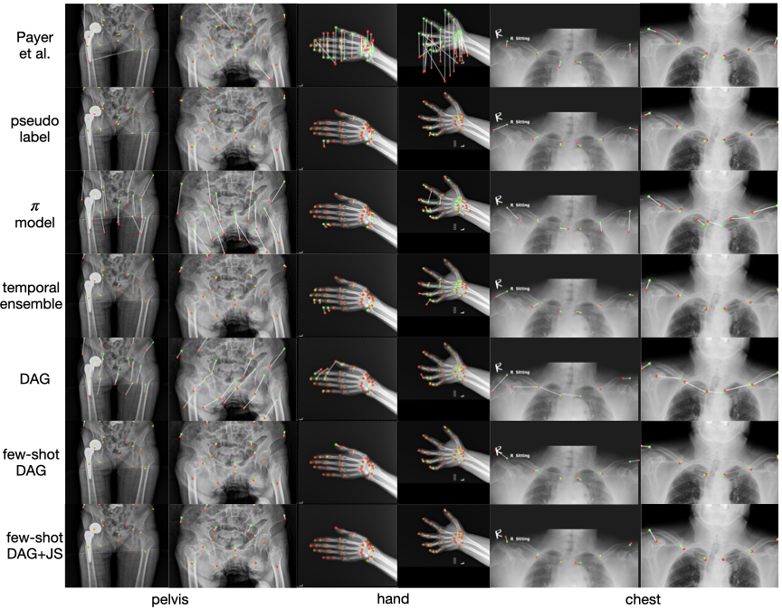
We select two examples for each data set and show the landmark localization results in Fig. 2. We can see that, Payer et al. and -Model generally performs unstably while pseudo label and temporal ensemble can achieve reasonable landmark localization except for a few hard cases, i.e., the second hand image. The fully-supervised deep adaptive graph can out-perform Payer et al., however, it under-performs strong semi-supervised methods, i.e., pseudo label and temporal ensemble. But, the proposed semi-supervised learning scheme (few-shot deep adaptive graph) and the Jensen–Shannon divergence loss (few-shot deep adaptive graph + Jensen–Shannon) can correct the less-optimal localization generated in fully-supervised deep adaptive graph and achieves the visually reasonable localization on all images including the hard cases.
4 Conclusion
In this paper, we introduced few-shot deep adaptive graph, an semi-supervised learning enhancement of deep adaptive graph that significantly improves landmark localization. It first trains a deep adaptive graph model on a few labeled training examples (e.g., five), and then fine-tunes the trained model on a large number of unlabeled training examples using consistency losses tailored for convolutional neural network and graph convolutional network outputs. Overall, our approach achieves strong landmark localization performances with only a few training examples. As shown in the validation on three datasets, the proposed few-shot DAG consistently out-performs both previous fully-supervised and semi-supervised methods with notable margins, indicating its good performance, robustness and potentially wide application in the future.
References
- [1] Berthelot, D., Carlini, N., Goodfellow, I., Papernot, N., Oliver, A., Raffel, C.A.: Mixmatch: A holistic approach to semi-supervised learning. In: Advances in Neural Information Processing Systems. pp. 5049–5059 (2019)
- [2] Cui, W., Liu, Y., Li, Y., Guo, M., Li, Y., Li, X., Wang, T., Zeng, X., Ye, C.: Semi-supervised brain lesion segmentation with an adapted mean teacher model. In: International Conference on Information Processing in Medical Imaging. pp. 554–565. Springer (2019)
- [3] Duchi, J., Hazan, E., Singer, Y.: Adaptive subgradient methods for online learning and stochastic optimization. Journal of machine learning research 12(7) (2011)
- [4] Han, D., Gao, Y., Wu, G., Yap, P.T., Shen, D.: Robust anatomical landmark detection with application to mr brain image registration. Computerized Medical Imaging and Graphics 46, 277–290 (2015)
- [5] Honari, S., Molchanov, P., Tyree, S., Vincent, P., Pal, C., Kautz, J.: Improving landmark localization with semi-supervised learning. In: Proceedings of the IEEE Conference on Computer Vision and Pattern Recognition. pp. 1546–1555 (2018)
- [6] Juneja, M., Garg, P., Kaur, R., Manocha, P., Batra, S., Singh, P., Singh, S., Jindal, P., et al.: A review on cephalometric landmark detection techniques. Biomedical Signal Processing and Control 66, 102486 (2021)
- [7] Laine, S., Aila, T.: Temporal ensembling for semi-supervised learning. arXiv preprint arXiv:1610.02242 (2016)
- [8] Lee, D.H.: Pseudo-label: The simple and efficient semi-supervised learning method for deep neural networks. In: Workshop on challenges in representation learning, ICML. vol. 3 (2013)
- [9] Li, W., Lu, Y., Zheng, K., Liao, H., Lin, C., Luo, J., Cheng, C.T., Xiao, J., Lu, L., Kuo, C.F., et al.: Structured landmark detection via topology-adapting deep graph learning. arXiv preprint arXiv:2004.08190 (2020)
- [10] Liu, C., Xie, H., Zhang, S., Mao, Z., Sun, J., Zhang, Y.: Misshapen pelvis landmark detection with local-global feature learning for diagnosing developmental dysplasia of the hip. IEEE Transactions on Medical Imaging 39(12), 3944–3954 (2020)
- [11] Lu, Y., Li, W., Zheng, K., Wang, Y., Harrison, A.P., Lin, C., Wang, S., Xiao, J., Lu, L., Kuo, C.F., et al.: Learning to segment anatomical structures accurately from one exemplar. In: International Conference on Medical Image Computing and Computer-Assisted Intervention. pp. 678–688. Springer (2020)
- [12] Lu, Y., Zheng, K., Li, W., Wang, Y., Harrison, A.P., Lin, C., Wang, S., Xiao, J., Lu, L., Kuo, C.F., et al.: Contour transformer network for one-shot segmentation of anatomical structures. IEEE Transactions on Medical Imaging (2020)
- [13] Lv, J., Shao, X., Xing, J., Cheng, C., Zhou, X.: A deep regression architecture with two-stage re-initialization for high performance facial landmark detection. In: Proceedings of the IEEE conference on computer vision and pattern recognition. pp. 3317–3326 (2017)
- [14] Payer, C., Štern, D., Bischof, H., Urschler, M.: Integrating spatial configuration into heatmap regression based cnns for landmark localization. Medical image analysis 54, 207–219 (2019)
- [15] Raju, A., Cheng, C.T., Huo, Y., Cai, J., Huang, J., Xiao, J., Lu, L., Liao, C., Harrison, A.P.: Co-heterogeneous and adaptive segmentation from multi-source and multi-phase ct imaging data: a study on pathological liver and lesion segmentation. In: European Conference on Computer Vision. pp. 448–465. Springer (2020)
- [16] Sohn, K., Zhang, Z., Li, C.L., Zhang, H., Lee, C.Y., Pfister, T.: A simple semi-supervised learning framework for object detection. arXiv preprint arXiv:2005.04757 (2020)
- [17] Sun, K., Xiao, B., Liu, D., Wang, J.: Deep high-resolution representation learning for human pose estimation. In: Proceedings of the IEEE/CVF Conference on Computer Vision and Pattern Recognition. pp. 5693–5703 (2019)
- [18] Tang, X., Guo, F., Shen, J., Du, T.: Facial landmark detection by semi-supervised deep learning. Neurocomputing 297, 22–32 (2018)
- [19] Tarvainen, A., Valpola, H.: Mean teachers are better role models: Weight-averaged consistency targets improve semi-supervised deep learning results. In: NeurIPS. pp. 1195–1204 (2017)
- [20] Trigeorgis, G., Snape, P., Nicolaou, M.A., Antonakos, E., Zafeiriou, S.: Mnemonic descent method: A recurrent process applied for end-to-end face alignment. In: Proceedings of the IEEE Conference on Computer Vision and Pattern Recognition. pp. 4177–4187 (2016)
- [21] Valle, R., Buenaposada, J.M., Valdes, A., Baumela, L.: A deeply-initialized coarse-to-fine ensemble of regression trees for face alignment. In: Proceedings of the European Conference on Computer Vision (ECCV). pp. 585–601 (2018)
- [22] Wang, Y., Zheng, K., Chang, C.T., Zhou, X.Y., Zheng, Z., Huang, L., Xiao, J., Lu, L., Liao, C.H., Miao, S.: Knowledge distillation with adaptive asymmetric label sharpening for semi-supervised fracture detection in chest x-rays. arXiv preprint arXiv:2012.15359 (2020)
- [23] Wu, W., Qian, C., Yang, S., Wang, Q., Cai, Y., Zhou, Q.: Look at boundary: A boundary-aware face alignment algorithm. In: Proceedings of the IEEE conference on computer vision and pattern recognition. pp. 2129–2138 (2018)
- [24] Wu, Y., Ji, Q.: Facial landmark detection: A literature survey. International Journal of Computer Vision 127(2), 115–142 (2019)
- [25] Yi, J., Wu, P., Huang, Q., Qu, H., Metaxas, D.N.: Vertebra-focused landmark detection for scoliosis assessment. In: 2020 IEEE 17th International Symposium on Biomedical Imaging (ISBI). pp. 736–740. IEEE (2020)
- [26] Yu, X., Zhou, F., Chandraker, M.: Deep deformation network for object landmark localization. In: European Conference on Computer Vision. pp. 52–70. Springer (2016)
- [27] Zhang, Z., Luo, P., Loy, C.C., Tang, X.: Learning deep representation for face alignment with auxiliary attributes. IEEE transactions on pattern analysis and machine intelligence 38(5), 918–930 (2015)
- [28] Zhu, M., Shi, D., Zheng, M., Sadiq, M.: Robust facial landmark detection via occlusion-adaptive deep networks. In: Proceedings of the IEEE/CVF Conference on Computer Vision and Pattern Recognition. pp. 3486–3496 (2019)