A Numerical Method to Find the Optimal Thermodynamic Cycle in Microscopic Heat Engine

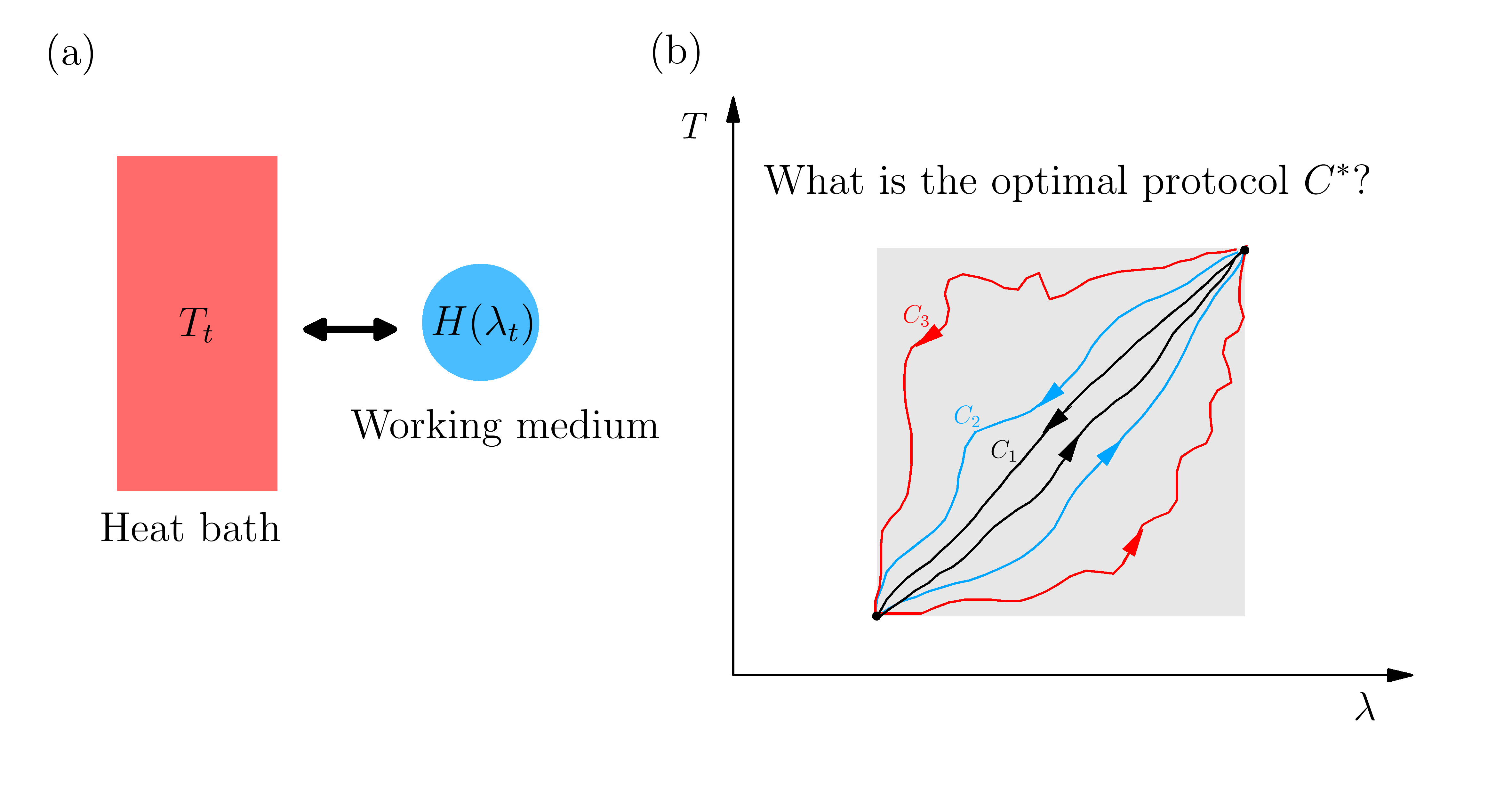
To apply the numerical method to the engine cycle, we need to fix the target function to optimize. In this paper, we consider the heat engine with slow driving parameters near quasi-static motion, where the adiabatic expansion from the instantaneous equilibrium state can formulate the thermodynamic quantities. We here introduce the theory in Ref.brandner2020thermodynamic which addresses the relation between the power and thermodynamic efficiency in heat engines with slowly varying parameters. As shown in Fig. 1 (a), we consider a microscopic heat engine which consists of a working medium with the Hamiltonian $H(\lambda)$ and a heat bath with the temperature $T$. Here, $\lambda$ is a time-dependent control parameter for the working medium, and the temperature also changes continuously in time. Both $\lambda$ and $T$ vary continuously and return to the original values after the period $\tau$ as shown in Fig. 1 (b). The heat engine cycle forms a closed path $C$ in the ($\lambda,T$)-plane. Note that in Fig. 1 (b) we especially fix the two points in the ($\lambda,T$)-plane, which will be discussed later in our numerical scheme.

We consider the time-dependent Markovian master equation for the density matrix $\rho_{t}$:

For instance, in the classical Brownian heat engine, one can employ the Fokker-Planck operator fokker1914mittlere for the operator $\mathbb{L}_{t}$. When we consider the quantum discrete system for the working medium, we can employ the Lindblad equation kossakowski1972quantum; lindblad1976generators; gorini1976completely. Following the standard framework of stochastic thermodynamics, the average work done by the working medium to the outer environment is written as follows

where $\tau$ is the period of the cycle. Throughout this paper, the Boltzmann constant is set to be unity. In addition, the effective heat uptake over the cycle is defined as

The functions $f_{t}^{\lambda}$ and $f_{t}^{T}$ are thermodynamic forces, which respectively play roles of the instantaneous generalized pressure and entropy of the working system.

When the heat engine cycle contains continuously varying temperatures, the conventional thermodynamic efficiency is not very convenient. Hence, instead, Ref.brandner2020thermodynamic introduced a more general definition on efficiency. Using the non-negativity of the entropy production rate and cyclic property, one can show the inequality $U-W\geq 0$. From this property, new efficiency $\eta$ is defined as

One can notice that $\eta$ is $1$ for reversible heat engines. The standard Carnot efficiency can be reproduced once suitably normalized for the engines with two temperatures such as the Carnot cycle brandner2020thermodynamic.

Near the quasi-static regime where the controllable parameters change very slowly, the periodic state $\rho_{t}$ can be expanded from the quasi-static limit $1/\tau\rightarrow 0$ as $\rho_{t}\approx\rho_{eq,t}+\delta\rho_{t}+\delta(1/\tau^{2})$, where $\rho_{eq,t}$ is the instantaneous equilibrium distribution, i.e, $\mathbb{L}_{t}\rho_{eq,t}=0$. The first order $\delta\rho_{t}$ is solved through the equation,

Substituting the expressions into the thermodynamic forces, one obtains the following linear response form,

where $f_{eq,t}^{T}$ and $f_{eq,t}^{\lambda}$ are thermodynamic forces of instantaneous equilibrium state. The matrix $\mathcal{R}$ is the adiabatic response matrix, which stands for the response against the perturbation from the instantaneous equilibrium state. The expression of the matrix elements in $\mathcal{R}$ depends on the choice of dynamics $\mathbb{L}_{t}$. Using this adiabatic expansion, it is shown in Ref.brandner2020thermodynamic, the power $P$ and efficiency $\eta$ has the following trade-off relation

where $\mathcal{W}$ is the quasi-static work for given cycle $C$, and the quantity $\mathcal{L}$ is the thermodynamic length defined as

The metric $g^{\mu\nu}$ is originally defined in the expansion of the function $U-W=\int_{0}^{\tau}dtg^{\mu\nu}\dot{\mu}\dot{\nu}$. The thermodynamic length is thought to be a measure of the minimal dissipation along the fixed contour $C$. The upper bound of power is linearly decreasing as the efficiency increases and its decreasing speed is determined by the combination of $\mathcal{W}/\mathcal{L}$. The quantity $\mathcal{W}/\mathcal{L}$ is purely geometrical quantity dependent solely on the given contour $C$.

It is known that the relation (9) is a tight bound for the power brandner2020thermodynamic. Once the cycle is determined, the upper bound can be obtained by changing the speed of protocol along the given contour $C$. It means that when $\mathcal{W}/\mathcal{L}$ is extremely large for a certain cycle, high efficiency and large power output of the heat engine can be obtained simultaneously using such cycle. Hence, in this paper, we consider the numerical method to find the optimal cyclic protocol $C^{*}$ in the ($\lambda,T$)-plane to maximize $\mathcal{W}/\mathcal{L}$ with several conditions, i.e.,

within the available parameter regime in the $\lambda-T$ plane. Concerning the available parameter regime, for simplicity, we fix the two points as shown in Fig. 1 (b), and the available parameter regime is assumed to be inside the square given determined by the two points (grey shaded regime). Although this setup is simple, there are infinite numbers of candidates as contours even in this limited regime, and hence the optimization is highly nontrivial. We propose a numerical method to solve this problem based on two models described in the subsequent sections.

As the first example, we consider the overdamped Brownian particle heat engine. The working system here is an one-dimensional classical overdamped Brownian particle in the time-dependent potential $V(x,\lambda_{t})$, where the quadratic potential $V(x,\lambda_{t})=\lambda_{t}x^{2}/2$ is applied. The temperature of the system is also continuously controlled in time. Then the dynamics of the distribution is described by the Fokker-Planck equation:

where $\rho_{t}(x)$ is the distribution of the particle at the position $x$ and time $t$. The instantaneous equilibrium state of the distribution is given by

where $\omega=\lambda/2T$. To solve Eq. (13) in the slow driving case near quasi-static motion, the distribution $\rho_{t}(x)$ is expanded up to the first order. The first order of the distribution is explicitly given as

The derivation of this expression is explained in the Appendix A. Inserting the expression (16) to the thermodynamic forces (4) and (5), the quasi-static generalized pressure $f_{eq,t}^{\lambda}$ and the adiabatic response matrix $\mathcal{R}$ in (8) are given as follows

From these expressions, one can arrive at the expression of the quasi-static work and thermodynamic length for the given cycle $C$

Another example we consider is the single-qubit heat engine. This model is also employed in Ref. brandner2020thermodynamic in a different context. The engine consists of a qubit surrounded by a thermal environment with controllable temperature $T$. The Hamiltonian of the qubit is

Here, $\sigma_{x}$ and $\sigma_{z}$ are Pauli matrices, $\hbar\Omega$ denotes overall energy scale, setting to be unity. The term $\varepsilon$ causes the quantum coherence and hence, the dynamics become classical once we set $\varepsilon=0$. The parameter $\lambda$ is time-dependent. We assume $\varepsilon\geq 0$ and $\lambda\geq\varepsilon$.

The equation of motion with respect to the density matrix $\rho_{t}$ of the qubit is described by the Lindblad equation

where $V^{\sigma}$ is the jump operator satisfying the quantum detailed balance condition, $[H_{\lambda},V^{\pm}]=\pm\hbar\Omega\lambda V^{\pm}$, and ${\rm Tr}\left[V^{\pm}V^{\pm{\dagger}}\right]=\pm\Gamma\Omega\lambda/\left[1-\exp{\left[\mp\hbar\Omega\lambda/T\right]}\right]$. From the adiabatic approximation, the quasi-static work $\mathcal{W}$ is given as brandner2020thermodynamic

We can calculate the thermodynamic length by Eq. (10). Especially for $\varepsilon=0$, the thermodynamic length is given by $\mathcal{L}_{d}$ brandner2020thermodynamic:

When $\varepsilon\neq 0$, we obtain different expressions containing the quantum effect. See brandner2020thermodynamic and Appendix B for the details.

It is interesting that $\mathcal{L}_{d}$ shows the similar expression to $\mathcal{L}$ of the classical Brownian heat engine (Eq. (20)). When thermodynamic length takes its minimum value 0, the absolute terms in both Eq. (20) and Eq. (24) are zero and give the differential equation,

One can solve this equation directly and find that $\lambda$ is linearly proportional to $T$, i.e., $\lambda=\kappa T$, where $\kappa$ is a time-independent constant. In this situation, the corresponding quasi-static work is also zero. This extreme situation is avoided by imposing a constraint on the adiabatic work ${\cal W}\geq{\cal W}_{0}>0$ as in (12).

The optimization problem (12) illustrated in section 2.2 is actually a two-dimensional variational optimization problem that is difficult to solve analytically. Instead, we deal with it numerically.

We impose the following constraints for the cycle. (i) The cycle should be a simple closed curve, which means that the curve has no intersections. Otherwise, the protocol can be regarded as several sub-cycles. (ii) As explained in the section 2.2, we impose the constraint that the cycle must pass through the point $A$ and $B$, and we limit an available region to a square region made by the two points (see Fig. 1 (b) or the grey region in Fig. 2). (iii) We also impose the condition that the quasi-static work along the cycle must be larger than a given constant, i.e., $\mathcal{W}\geq{\mathcal{W}}_{0}$.

Concerning the constraint (ii), the available regime $D$ is mathematically described as

Because controllable parameters, such as the temperature $T$ and strength of potential or shifting energy $\lambda$, are usually finite. Note that even we limit the available regime as above, finding an optimized cycle is highly nontrivial.

Based on the above constraints on the cycle, we employ the following parametrizing method. See the schematic graph in Fig. 2. Assume that the optimal cycle $C^{*}$ must path through two corners of the available square regime $D$: $A(1,1)$ and $B(2,2)$ which divide the path into two parts, $C_{1}:A\rightarrow B$ and $C_{2}:B\rightarrow A$. We then map the closed curve $C^{*}$ into an unclosed curve $C^{\prime}$ by the following coordinate transformations (See Fig. 2, again). We first translate coordinates so that $A$ can overlap with the origin, and rotate them $\pi/4$ counterclockwise to ensure that $B$ lies in the horizontal axis. Next, we fold the part $C_{2}$ into $C_{2}^{\prime}$ centered on $B$. Thus, $A$ is folded to the other side of $B$ along the horizontal axis. After zooming, the intersects between the new curve $C^{\prime}$ and the horizontal axis are $A^{\prime}(0,0)$, $B^{\prime}(1,0)$ and $A^{\prime\prime}(2,0)$. Then, $\lambda$ and $T$ can be expressed by the new coordinates $x$ and $y$, i.e.,

and

where $C_{1}^{\prime}$ and $C_{2}^{\prime}$ respectively corresponds $C_{1}$ and $C_{2}$ in original curve. We can express them respectively by functions of $x$, $g_{1}(x)$ and $g_{2}(x)$. The total quasi-static work and thermodynamic length can then be expressed as the summations of the quasi-static works and thermodynamic lengths for $C_{1}$ and $C_{2}$ respectively. Thus, our optimization problem becomes finding the optimal $g_{1}(x)$ and $g_{2}(x)$ to maximize $\mathcal{W}/\mathcal{L}$, i.e.,

where $\mathcal{W}_{m}$ and $\mathcal{L}_{m}$ ($m=1,2$) are the quasi-static works and the thermodynamic lengths for the contour $C_{m}$, respectively.

In addition, we use the Fourier representation for the functions $g_{m}(x)~(m=1,2)$:

Finding optimal path now reduces to finding the Fourier components, and hence the corresponding $\mathcal{W}_{m}$ and $\mathcal{L}_{m}$ is respectively parametrized by $\bm{b}^{(m)}$ as $\mathcal{W}_{m}(\bm{b}^{(m)})$ and $\mathcal{L}_{m}(\bm{b}^{(m)})$.

Finally, we write the constraints (i), (ii) and (iii) in terms of the functions $g_{m}(x;\bm{b}^{(m)})$. Note that without loss of generality, we choose the condition that $g_{1}(x)\leq 0$ and $g_{2}\geq 0$ to satisfy the Constraint (i). Then, the expressions for the constraints can be written as follows

Consequently, our optimization problem (12) is reduced to finding the optimal parameters $\bm{b}^{(m)}$ under constraints (31) to maximize $\mathcal{W}/\mathcal{L}$, i.e.,

Studies of computer sciences provided many optimization algorithms to solve the problem above. In this paper, we use the Genetic Algorithm (GA) with penalty functions. GA is an optimization method via simulating the natural selection whitley1994genetic, which is originally inspired by the process of natural selection and biological evolution based on genetic mechanism. Focusing on all individuals in a population, GA randomly searches the optimal solution in coded parameter space. This gives its well global searching ability. To establish GA on our problem, the following five parts are needed to be carefully considered, including parameter-coding, initialization, design of fitness function and genetic operations (selection, crossover, and mutation), and settings of control parameters.

First, we consider the parameter-coding process. For our problem, the parameter vector to be optimized is $\bm{b}^{(m)}$. Thus, one can uniquely specify some imaginary creature by the values of $\bm{b}^{(m)}$. Similar to the gene sequence in the real world, if one regards $\bm{b}^{(m)}$ as the unique character of the imaginary creature, its binary notation vector $\hat{\bm{b}}^{(m)}$ then can be regarded as the corresponding unique gene sequence. The length of the binary notation can be adjusted by a factitiously determined precision $\Delta$.

Second, in order to simulate the natural selection process, a population which consists of $N$ arbitrary imaginary creature is needed. Initially, it is a set of randomly-selected parameter vectors, i.e., $G=\{\hat{\bm{b}}_{1}^{(m)},\hat{\bm{b}}_{2}^{(m)},...,\hat{\bm{b}}_{N}^{(m)}\}$.

Third, natural selection process obsoletes the creature according to its fitness, which is described by the fitness function in GA. Basically, the fitness function is often set to be the target function. For our problem, considering the constraints (31), we transform the problem (32) into the following one without constraints with the help of penalty function method,

Here, $P(\bm{b}^{(m)})$ is the penalty function,

by equally dividing the range $[0,2]$ of $x$ with $n_{c}$ points. $\sigma$ is a large penal constant. Hence, the fitness function in our problem is set to be $F(\bm{b}^{(m)})$. In the selection step, we calculate $F(\bm{b}^{(m)})$ for every creature in the population $G$. If some creature has a low value of fitness, it may die out with a larger probability than others. We select $N_{s}$ creatures in $G$ to survive. Please see Appendix D for details.

Moreover, in order to adapt to the environment, these $N_{s}$ surviving creatures must reproduce their children. Parents are equally randomly selected in the surviving creatures and a pair of parents can only reproduce one child. By gene mutation and gene crossover process, genes in children can be optimized. In situations considered in this paper, two random sites of each dimension of the binary notation vector $\hat{\bm{b}}^{(m)}$ are selected to be the crossover points on both parents’ gene sequences, and each fragment divided by the selected sites has a probability to be inherited by their child. In the gene mutation process, random sites of each dimension of the binary notation vector $\hat{\bm{b}}_{1}^{(m)}$ has a probability to change to its opposite value ($0$ or $1$) only. Please see Appendix E for details.

Thus, the remaining $N_{s}$ parents and the new $N-N_{s}$ child make up the new population. After enough such iterations, the process of natural selection ensures that the fitness of each individual in the population can be optimized.

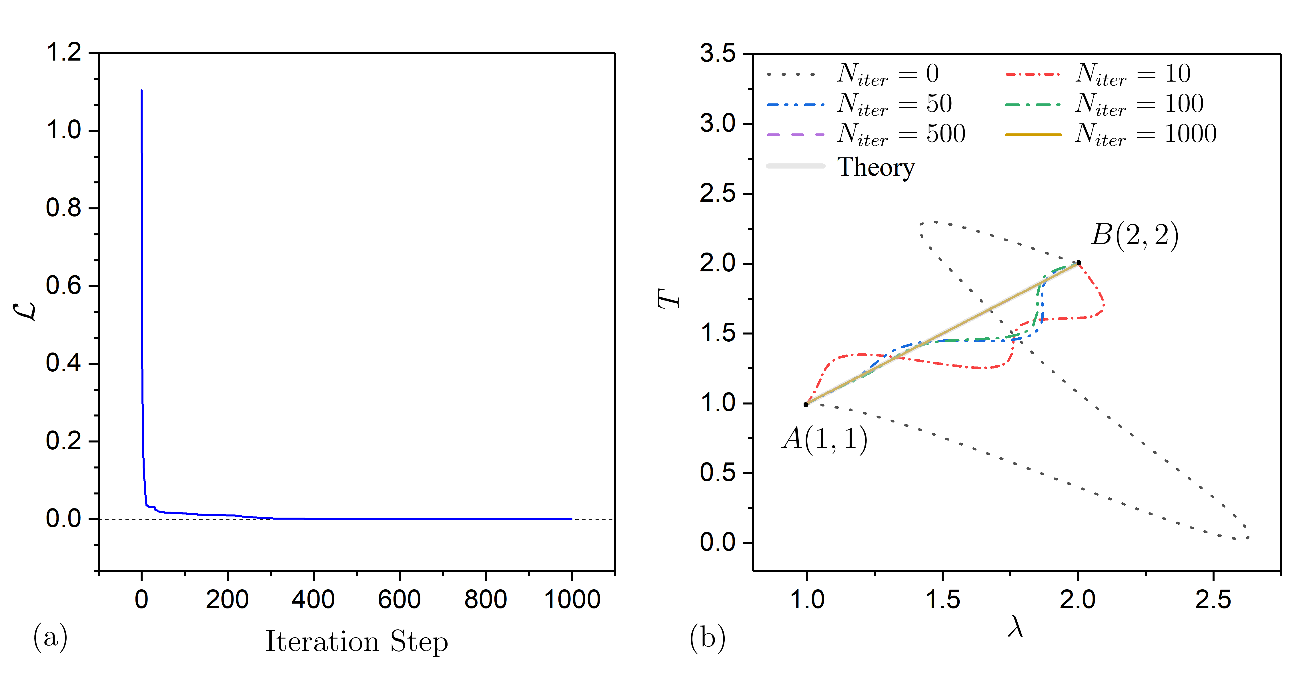
To demonstrate that the GA can correctly find the optimal solution for our problem, we present an analytically solvable problem in this section. The problem is to find the optimal protocol $\gamma^{*}$ in the parameter plane $\lambda-T$ from $A(1,1)$ to $B(2,2)$ that minimizes the minimum thermodynamic length $\mathcal{L}$. We consider this problem for the classical overdamped Brownian particle, i.e.,

As discussed in Section 2.2, we can theoretically find the optimal path $\gamma^{*}$. The solution is a simple line $T=\lambda$, where the corresponding minimum thermodynamic length $\mathcal{L}^{*}=0$. Numerically, we deal with this problem by employing the parametrization method and the GA above. Instead of considering the whole cycle, we only need to parametrize half of it (i.e., $C_{1}$) like the form of Eq. (31). Besides, we do not have any constraints on $\gamma$ here. Results are shown in Fig. 3. One can notice that as the iteration steps increases, the protocol gradually converges to the theoretical solution (Fig. 3 (a)) and the target function $\mathcal{L}$ converges to the theoretical prediction $0$ (Fig.3 (b)). It indicates that our method with the GA is reliable.

We first show the results for the Brownian heat engine. In this case, we set a finite constraint on the quasi-static work, i.e., ${\cal W}\geq{\cal W}_{0}~(>0)$. Fig. 4 (a) shows a numerical saturation as a function of iteration steps. One can notice that the target function $F$ converges to some constant after sufficient large iteration steps for each situation. Here, we use the same random seed in the numerical calculation as an initial state, and hence, different curves overlap for different $\mathcal{W}_{0}$ at small iteration steps in Fig. 4 (a). In Figs.4 (a), (c) and (d), we use the Fourier modes $n=10$, which is enough for accuracy, as indicated in Fig. 4 (b).

Once target functions converge, optimal thermodynamic cycles can be obtained, which are shown in Fig. 4 (c). We also show the saturated values of ${\cal W}/{\cal L}$, ${\cal L}$, and ${\cal W}$ as a function of constraint ${\cal W}_{0}$ in Fig. 4 (d). We discuss these results. As shown in Fig. 4 (c), by imposing the constraint on the quasi-static work $\mathcal{W}$, one can see that as increasing the constraint ${\cal W}_{0}$, the optimal cycle approaches to the boundary of $D$ which is the allowable maximum cycle in the domain. This supports the intuition that a large work ${\cal W}$ requires a large area.

The work $\mathcal{W}$ reaches its maximum value ($\sim 0.32$) shown in Fig. 4 (d). The available domain $D$ plays the role of an upper bound on the quasi-static work. To produce the maximum work and maximum $\mathcal{W}/\mathcal{L}$ simultaneously, the heat engine is required to be operated inside the boundary of $D$. Particularly, if $\mathcal{W}_{0}$ exceeds the upper limit ($\sim 0.32$), i.e., the constraint $\mathcal{W}\geq\mathcal{W}_{0}$ is no longer applicable. In this case, the term $\sigma\left|\max(0,\mathcal{W}(\bm{b}^{(m)})\right|$ in the penalty function (34) can never be avoided. Our algorithm can still minimize the target function $F$ and reduce the penal term above as much as possible. The consequence of this trend is that the quasi-static work can still be maximized to the upper limit, but the corresponding optimal cycle will no longer change. This is why the cycles overlap with each other when $\mathcal{W}_{0}>0.32$ in Fig. 4 (c).

By imposing a large constraint ${\cal W}_{0}$ as above, one can see that a large area in the cycle is generally necessary for large adiabatic work ${\cal W}$. On the other hand, we also need to note that a small area in the cycle is required for a small thermodynamic length ${\cal L}$. Hence, in general, there is a sort of trade-off between obtaining large ${\cal W}$ and reducing ${\cal L}$. As decreasing the constraint ${\cal W}_{0}$, the effects arising from this trade-off become significant. Let us discuss the regime of ${\cal W}_{0}<0.32$ in the bottom figure of Fig. 4 (d). The figure shows that in this regime, the quasi-static work along the optimal cycle tends to equal $\mathcal{W}_{0}$. It is also equivalent to that our algorithm tries to obtain a small area of the engine cycle, which leads to small values of ${\cal L}$. Hence, the numerical results non-trivially show that to obtain the maximizing the rate ${\cal W}/{\cal L}$, obtaining small adiabatic work $\mathcal{W}$ is a good strategy. This also implies that the constraint on $\mathcal{W}$ limits the maximum value of $\mathcal{W}/\mathcal{L}$ in this regime. We also notice that the corresponding optimal cycle also gradually shrinks from the boundary (the cases ${\cal W}_{0}=0.18,0.24$ and $0.30$) in Fig. 4 (c). We believe that this behavior appears as a result of nontrivial trade-off properties to ${\cal W}/{\cal L}$.

Until $\mathcal{W}_{0}\leq 0.17$, flat behavior appear again in the graph of $\mathcal{W}$, $\mathcal{L}$ and $\mathcal{W}/\mathcal{L}$. These platforms indicate that there will be no optimal cycle better than that of $\mathcal{W}=0.17$, i.e., the cycle we obtain here is the global optimal cycle that can maximize $\mathcal{W}/\mathcal{L}$ in domain $D$.

We now recall that the value $\mathcal{W}/\mathcal{L}$ determines whether the large power and large efficiency can be obtained simultaneously, as shown in the general theory (9). As shown in Fig. 4 (d), the maximum value of $\mathcal{W}/\mathcal{L}$ is about $0.40$, which is finite, and hence large power and large efficiency cannot be obtained simultaneously in this system. However, we stress that based on our approach, one can systematically find the optimum cycle for the Brownian heat engine.

We next show that our numerical scheme also works well in the single-qubit heat engines. In this case, we can consider the effect of the quantum coherence $\varepsilon$ in the dynamics. Hence, we consider two cases, i.e., the classical case and the quantum case. In the classical case, we set the quantum coherence $\varepsilon$ to zero in the Hamiltonian (21), and we set a finite constraint on the adiabatic work. In the quantum case, we set a finite value for the quantum coherence $\varepsilon$, and we do not impose a constraint on the adiabatic work, i.e., ${\cal W}_{0}=0$.

We first discuss the classical case $\varepsilon=0$. The results are shown in Fig. 5. We use the Fourier mode $n=10$, which does not cause significant errors, as can be seen in Fig. 5 (b). This indicates that our numerical scheme works well even in discrete level heat engines. Regarding the behavior of cycles, a similar conclusion to the Brownian heat engine can be given. Our numerical calculation shows that the value of $\mathcal{W}/\mathcal{L}$ is always finite, which implies that the large power and large efficiency cannot be obtained simultaneously, similarly to the Brownian heat engine case.

We next look at the quantum case, i.e., $\varepsilon\neq 0$. We can see that our method works well as shown in Figs. 6(a) and (b). As indicated in Fig. 6, the quantum coherence factor $\varepsilon$ automatically provides a constraint on $\mathcal{W}$ when maximizing $\mathcal{W}/\mathcal{L}$, which reduces the performance of the heat engine. This is consistent with Brander and Saito’s conclusion for the example cycle they introduced brandner2020thermodynamic. For the available $\lambda$-$T$ plane, our numerical algorithm clarifies the best heat engine cycle even in the quantum case.