On the Design and Analysis of Multivariable Extremum Seeking Control using Fast Fourier Transform
Abstract
This paper proposes a multivariable extremum seeking scheme using Fast Fourier Transform (FFT) for a network of subsystems working towards optimizing the sum of their local objectives, where the overall objective is the only available measurement. Here, the different inputs are perturbed with different dither frequencies, and the power spectrum of the overall output signal obtained using FFT is used to estimate the steady-state cost gradient w.r.t. each input. The inputs for the subsystems are then updated using integral control in order to drive the respective gradients to zero. This paper provides analytical rules for designing the FFT-based gradient estimation algorithm and analyzes the stability properties of the resulting extremum seeking scheme for the static map setting. The effectiveness of the proposed FFT-based multivariable extremum seeking scheme is demonstrated using two examples, namely, wind farm power optimization problem, and a heat exchanger network for industrial waste-to-heat recovery.
1 Introduction
Extremum seeking control (ESC) has emerged as a popular real-time optimization (RTO) and adaptive control tool to optimize the steady-state output of a plant, despite lack of a mathematical model. The most popular approach to estimating the gradient is the classical sinusoidal perturbation-based extremum seeking control that dates back to the work of Draper and Li [1], and later gained popularity with the work of Krstic and Wang [2]. The classical extremum seeking control is based on perturbing the input with a slow sinusoidal dither signal, such that the plant appears as a static map. A high-pass filter is used to remove the DC-component of the cost measurement, and the resulting detrended sinusoidal response of the output signal (with zero mean) is correlated with the perturbation signal. The product of the two sinusoids will have a DC component, which is extracted using a low-pass filter. This is approximately the steady-state cost gradient as explained in [2, 3]. The classical extremum seeking control thus involves the use of a high-pass and low-pass filter such that the dither signal is in the pass band of the filters [3].
Although extremum seeking control was historically developed for single-input single-output (SISO) systems, there has been several developments in extremum seeking control for large-scale networks with many subsystems, with applications ranging from wind farm power optimization[4, 5, 6, 7], maximum power point tracking for photovoltaic grids [8, 6], oil production network [9, 10], heat exchanger networks [11, 12], formation flight control [13] etc. to name a few. Development of extremum seeking control for such multi-input systems can be broadly categorized into multivariable ESC and distributed ESC.
Multivariable extremum seeking control considers a multi-input single-output (MISO) case, where the objective is to estimate the steady-state gradient of the overall cost w.r.t. each input [8, 14]. Distributed extremum seeking on the other hand assumes that each subsystem in the network has access to its local cost measurement. Each subsystem then locally employs single-input single-output (SISO) extremum seeking loop, and a consensus estimation algorithm is used for coordination among the different subsystems as explained in [15, 16, 4]. This paper deals with the former class, where we assume that the different subsystems in a network work towards optimizing the sum of their local objectives, however the local cost of each subsystem is not available. Maximizing total power generation from a wind farm or photovoltaic grid, maximizing oil and gas production from a network of wells, maximizing heat recovery in a heat exchanger network, minimizing total energy consumption in a processing plant or in a commercial building are a few examples of such systems.
As noted in [2, 3], the choice of the filter cut-off frequencies in the classical extremum seeking approach depends on the input perturbation frequency. With multiple inputs and a single output, tuning and designing the filter cut-off frequencies to retrieve the gradient w.r.t each input channel from the single cost measurement may not be trivial in practice. This is due to the fact that the output signal now contains the frequency components of the different input perturbations. Moreover, using the same low-pass filter on each channel may also lead to additional harmonics in the gradient estimation as noted in [8]. In short, good performance of the multivariable extremum seeking control using this approach requires good tuning of the filter cut-off frequencies, which can be challenging and time consuming, especially in large-scale networks with several inputs.
A natural and systematic approach to analyze the effect of different frequency components in a signal is to use the Fourier transform for spectral analysis, which maps the time series data into a series of frequencies. The underlying idea behind the proposed multivariable FFT-based extremum seeking scheme is as follows: For a static map as shown in Fig. 1, at a sinusoidal perturbation in the input , generates a sinusoidal variation in the output at the same frequency . The power spectrum of the output signal would then have an amplitude of at frequency . Similarly, for , a sinusoidal perturbation in the input , generates a sinusoidal variation in the output at the same frequency shifted by 180∘ resulting in . Also in this case, the power spectrum of the output signal would have an amplitude of at . For , a sinusoidal perturbation in the input , generates a periodic signal with twice the frequency. Consequently, the power spectrum would indicate an amplitude of zero at , since the power of the signal at this frequency is zero. Instead the power spectrum would have a non-zero amplitude at . For example, if we have a quadratic static map , adding at would result in an output variation of , which clearly only has a frequency component at . The amplitude spectrum, which shows the strength of the variations of a signal at different frequencies is thus a very good indicator of the gradients at the different perturbation frequencies. Another advantage of using FFT-based extremum seeking is that it is robust to slowly varying unmeasured disturbances as long as they are not in the same frequency as any of the input perturbations.

In the context of extremum seeking control, Fourier transform has been predominantly used to extract the phase information in order to compensate for the phase shift introduced by the plant dynamics, such that the static map assumption can be relaxed [17, 18, 19]. For example, the authors in [18] estimate the different harmonics using a Kalman filter, and drive the high frequency harmonics to zero when the perturbation and the plant dynamics are in the same timescale. On the other hand, in this paper we use FFT to directly extract the gradient information w.r.t multiple input channels from the amplitude spectrum using the two-timescale separation principle (just as in the case with classical extremum seeking control). The phase spectrum may be used only to estimate the sign of the gradient. The intuitive nature of FFT and the amplitude spectrum has previously led to the use of gradient estimation using FFT in a few engineering applications such as [20, 21]. However, these works provide little information into designing the FFT-based extremum seeking scheme and analyze its properties, which this paper aims to address.
To this end, this paper formalizes the multivariable extremum seeking scheme using fast Fourier transform (FFT) and studies its stability properties. In particular, the main contribution of this paper is to provide analytical rules on the choice of the tuning parameters, namely, the window frame length , and the integral gain that ensures closed-loop stability of the proposed FFT-based extremum seeking scheme. The effectiveness of the FFT-based extremum seeking scheme is demonstrated using a wind farm optimization example, as well as on a industrial waste-to-heat recovery network.
2 Extremum seeking control using Fast Fourier Transform (FFT)
Consider a network of subsystems working towards optimizing the sum of their local objectives The inputs are denoted by , and the overall cost function is denoted by the static map where denotes the unknown functions representing the local cost for each subsystem . The objective is to minimize the overall cost of the network
| (1) |
Assumption 1.
The overall cost measurement is additively separable, but the local cost measurements are not available.
The above assumption implies that we consider a multi-input single-output (MISO) plant. Without loss of generality, we state the following assumption for a minimization problem.
Assumption 2.
The nonlinear map is sufficiently smooth and continuously differentiable with a unique minimum at , such that
| (2a) | ||||
| (2b) | ||||
| Furthermore such that | ||||
| (2c) | ||||
where
In this paper, we study the multivariable extremum seeking control of such a process, without the need for a mathematical model of the plant. The objective is to steer the system to the equilibrium using only the overall cost measurement .

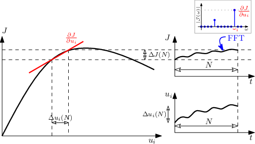
Each input channel is superimposed with a unique sinusoidal dither signal , with amplitude and frequency . The overall output cost measurement is then composed of the frequency components , for all . Using spectral analysis we can decompose the output signal into different frequency components. To do this, we use a sliding window of fixed length with past data points to get the point DFT using the finite set of cost measurement , and input signals for all . To perform FFT, the signals need to be detrended such that they have zero mean. Hence, the DC-component from the time domain data is removed, for example by using a moving average filter. The detrended signals with zero-mean are denoted by the superscript .
Remark 1.
The detrending step is analogous to the high pass filter in the classical extremum seeking control, where the purpose of the high pass filter is also to remove the DC component from the cost measurement [2].
Let the past discrete samples of the detrended output cost measurement , be denoted by . The discrete-time Fourier transform (DTFT) reads as and the -point DFT samples at frequency components given by,
| (3) |
is a complex valued function, which has a corresponding magnitude spectrum denoted by , and a phase spectrum denoted by . The magnitude of the cost function for the input dither frequencies for all can then be obtained from the single-sided amplitude spectrum for all , where we extract the frequency components of interest from the -point DFT. That is, the magnitude of the cost gradient w.r.t. the input channel is given by
| (4) |
Hereafter, we denote simply as for the sake of notational simplicity. Since the amplitude spectrum , the phase information with respect to the phase of the input signal is used to determine the sign of the gradient. The phase is obtained from the FFT, and similarly, the phase of the input perturbations can be obtained using FFT of the dither signals.
Together, the gradient of the cost w.r.t to the input is then estimated as follows:
| (5) |
This is schematically shown in Fig. 2(a) for the input, where spectral analysis of the cost measurement from the past samples is used to estimate the local gradient . Alternatively, the estimated gradient can equivalently be computed directly as
| (6) |
where denotes the real part of a complex number, and is the DFT of the input signal.
Remark 2.
The Euler’s formula establishes the fundamental relationship between the complex exponential function and the trigonometric functions in (3). Thus, the product of the detrended cost and exponential terms in (3) can be seen as analogous to the product of the detrended output signal and the sinusoidal dither in classical extremum seeking control, which provides the demodulation effect at the perturbation frequency.
Once the gradient is estimated, the inputs can be updated using a gradient descent step, which is simply an integral controller to drive the estimated gradients to zero,
| (7) |
where is the integral gain for the input. The perturbation signals are added to the nominal input computed by the integral controller, and the resulting input is applied on the plant. The sketch of the proposed FFT-based extremum seeking control is shown in Algorithm 1.
3 Stability Analysis
Assumption 3 (Choice of dither signal).
- (i)
The output signal is persistently exciting of at least order .
- (ii)
is chosen such that the plant can be assumed to be a static map.
Assumption 3(i) can be satisfied if the perturbation frequencies of the different input channels are mutually independent, i.e. , , for any distinct , , and . This means that the frequency of one input perturbation must not be the same or lie in the harmonics of perturbation of the other input channels. This is to ensure that unique persistence of excitation condition is satisfied [14]. With Assumption 3(ii) we restrict our analysis in this section to the static map setting, where the dynamics of the extremum seeking scheme are governed by (7).
When we use an -point DFT to obtain the amplitude spectrum, it is based on spectral analysis on a finite set of data with length . The choice of the window length is an important factor which affects the accuracy of the gradient estimation. If is not carefully chosen, then it is possible that the -point DFT may not sample the DTFT precisely at one or more of the perturbation frequencies. That is, the discrete frequency array may not contain one or more of the perturbation frequencies exactly (cf. (4)). This leads to spectral leakage resulting in bias in the spectral values, and consequently bias in the estimated gradient. The choice of the window length and its effect on the gradient estimation is formalized in the following theorem.
Theorem 1 (Minimum window length ).
Given assumption 3, the length of the moving window frame that ensures no spectral leakage in the N-point DFT of the output signal is given by
| (8) |
for some and where denotes the least common multiple.
Proof.
We can consider the finite segment of a signal as a product of an infinite time series and a rectangular data window
The Fourier transform of is then given by
where denotes convolution. For a rectangular window, we have
where the periodic sinc function has mainlobes and sidelobes in the DTFT. Sampling this at for one can see that
which implies that the sidelobes are sampled at their zero values. Convolution with the sinusoidal signal gives a frequency-shifted periodic sinc centered around scaled by the amplitude . By choosing as (8) we ensure , and the integer number of cycles for all the frequency components within the samples ensures that there is no spectral leakage to nearby DFT bins [22, 23]. ∎
An alternative proof of Theorem 1 can be given by looking at the -point DFT in (3), where it can be seen that this is periodic with period . The inverse DFT of (3) expressed as
| (9) |
tells us that the reconstructed time series is also periodic with period . This is because sampling in the time domain results in periodicity in the frequency domain, and vice versa as given by the DFT sampling theorem. This implies that the two end points of the time series samples, and , are interpreted as though they were connected together [23, Ch. 5]. Therefore, by choosing as the least common multiple of the perturbation time periods (8), we can reconstruct that contains integer number of full time periods of all the perturbation frequencies . If is not chosen according to (8), then the reconstructed contains discontinuities, which results in higher order harmonics in the power spectrum. In this case, the DFT samples the sidelobes of the DTFT at non-zero values leading to spectral leakage. Furthermore, spectral leakage due to signals with non-integer number of cycles can also spread to other frequencies and can mask other signals, especially if their amplitude is relatively small, causing gradient estimation errors w.r.t other inputs as well. Therefore to avoid such issues, the minimum window length is given by (8) with in the FFT-based gradient estimation scheme.
Remark 3 (Minimum resolution).
In the multivariable setting, when we have several frequency components, the difference between any two perturbation frequencies and must satisfy
| (10) |
in order for it to be distinguishable in the amplitude spectrum. This is due to the windowing effect, where the DTFT has mainlobes which has a width of approximately [23].
Remark 4.
Due to the local linear approximation within the window, using the past data samples obtained at time , may lead to some deviations in the estimated gradient from the true gradient as the nominal input changes. See the simple illustrative example in Appendix A that clearly demonstrates this. The gradient estimation error due to the moving window is formalized in the following Lemma.
Lemma 1 (Boundedness of the gradient estimation error [27]).
Consider the FFT-based gradient estimation scheme given by (3)-(5), where the gradient estimated using the past data samples is denoted as . Let the true steady-state cost gradient w.r.t the inputs be denoted as . Given Assumptions 1, 2, and 3, and chosen according to Theorem 1, the gradient estimation error
| (11) |
is bounded by,
| (12) |
where is the Hessian of the static map.
Proof.
It is also intuitively understood that the error bound is higher for large as shown in (13). From (11) and (12) it can be seen that the gradient estimation error depends on the true gradient occurring somewhere in the last samples. This can be seen as a time delay, and in order to study the stability properties with time delay, we apply the Razumikhin condition to the Lyapunov stability analysis [28]. Given a positive definite function , the Razumikhin condition states that a time delay system with maximum time delay is asymptotically stable if there exists a continuous non-decreasing function , such that
| (15) |
Theorem 2 (Stability).
Proof.
To analyze the stability of the optimum , consider the candidate Lyapunov function,
| (16) |
with , and the derivative is written as,
Upper bounding the Hessian by and using Lemma 1, we can write this as
| (17) |
where the last inequality comes from (2c) in Assumption 2, which implies . Let for some , then using the Razumikhin condition (cf. (15)), for asymptotic stability we require if
Using this in (17), we get
For , we need , and since this is a minimization problem, we need in (7). Therefore, , if for all
∎
To summarize, Theorem 1 provides a lower bound on the length of the window frame as a function of the different input perturbation frequencies such that the gradient w.r.t all the inputs can be retrieved exactly from the amplitude spectrum of the output signal, and Theorem 2 provides bounds on the controller gains for each input channel such that the closed-loop system is stable under the static map condition.
4 Case Example: Wind farm optimization
In this section, we present a wind farm optimization example that demonstrate the performance of the proposed FFT-based gradient estimation scheme. The simulation results were performed in MATLAB v2020b, and the code can be found in the GitHub repository [29]. In this example, we consider a wind farm with identical wind turbines as shown in Fig. 3. We assume the wind direction is along the co-ordinate and orthogonal to the co-ordinate, as shown in Fig. 3. The wind turbines are uniform with diameter and blade roughness coefficient . The wind is in the direction of the positive -axis with a steady wind velocity of . The reader is referred to [30] for the wind farm model used in the simulation.
The wake interaction within a wind farm can significantly affect the overall power generation. The objective is thus to compute the optimal axial induction factor for the wind turbines , such that the total power generation from the wind farm is maximized. We assume that the total power produced by the wind farm is the only measurement available.


We set the initial axial induction factors to for all the wind turbines. The six inputs channels are superimposed with sinusoidal signals with frequencies and amplitude 0.003. The window length was chosen to be of 128 samples, according to Theorem 1.
The simulation results with the proposed FFT-based multivariable extremum seeking control is show in Fig. 4(a), where it can be seen that the proposed approach is able to drive the different inputs to the optimum such that the total power generated by the wind farm is maximized. Fig. 4(b) shows the spectrogram, where it can be seen that the amplitude of the power spectrum at the perturbation frequencies become zero as the system converges to the optimum. The same simulation results are repeated when the total power measurement is corrupted with a measurement noise of MW. The time series as wells as the spectrogram for this case is shown in Fig. 5.
4.1 Example 2: Maximizing heat recovery from a heat exchanger network
Consider an industrial cluster with different processing plants, the details of which are not important. The different processes in the industrial cluster generates some amount of surplus heat, which is to be recovered using a heat exchanger network, and transferred to a local district heating system, as shown in Fig. 6.

The cold stream inlet is split into eight different streams, one for each company in the industrial cluster. The objective here is to adjust the split ratio for each stream in order to maximize the total heat recovery, which can be equivalently stated as maximizing the end temperature of the cold stream [31]. The optimization problem can then be stated as,
| (18) |
where and .
As the temperature and flow rate of the hot stream from the industrial cluster varies, or if the overall heat transfer coefficient in the heat exchanger changes (e.g. due to heat exchanger fouling), this requires adjusting the split ratios in order to maximize the temperature. This process is inspired by the batch reactor heat recovery challenge problem from [32], where the authors considered a similar problem, and later proposed the concept of controlling the so-called Jäschke Temperature [31] in order to achieve optimal operation. The Jäschke Temperature is essentially the model gradient based on a simplified countercurrent heat exchanger model with arithmetic mean temperature difference.
In this industrial symbiosis network, we assume that no information regarding the heat exchanger network such as temperatures, flow rate, heat transfer coefficient etc. are available, and the model of the system is also not available. The end temperature is the only measurement that is available for online process optimization. Note that one does not even need to know if the heat exchangers are of countercurrent or concurrent type. The details of the simulator model used in this section can be found in Appendix C. Note that this model is only used to simulate the process and no knowledge of this model is used by the extremum seeking controller.
We set the initial split ratios to for . The temperature of the hot streams are initially C. After 2000 time steps, the temperature of the first hot stream increases to C. The seven inputs channels are superimposed with sinusoidal signals with frequencies and amplitude 0.003 for and for . The window length was chosen to be of 128 samples according to Theorem 1. The integral gain was chosen to be for all . The simulation results with the proposed FFT-based multivariable extremum seeking control is show in Fig. 7, where it can be seen that the proposed approach is able to drive the different inputs to the optimum such that the end temperature supplied to the district heating is maximized.

5 Conclusion
This paper presented a multivariable extremum seeking scheme, where the gradient is estimated using spectral analysis obtained using fast Fourier transform (FFT) as shown in Algorithm 1. The proposed approach requires relatively less tuning parameters compared to the classical extremum seeking control. The choice of the window length is formalized in Theorem 1. Lemma 1 showed that the gradient estimation error due to a moving window length is bounded and Theorem 2 provides bounds on the gain such that the algorithm asymptotically converges to the optimum in the static map setting.
Acknowledgments
Useful discussions with Prof. Sigurd Skogestad at the Norwegian University of Science and Technology, as well as with Dr. Pål Kittilsen at Equinor Research Center are gratefully acknowledged.
References
- [1] C. S. Draper and Y. T. Li, Principles of optimalizing control systems and an application to the internal combustion engine. American Society of Mechanical Engineers, 1951.
- [2] M. Krstić and H.-H. Wang, “Stability of extremum seeking feedback for general nonlinear dynamic systems,” Automatica, vol. 36, no. 4, pp. 595–601, 2000.
- [3] Y. Tan, W. Moase, C. Manzie, D. Nešić, and I. Mareels, “Extremum seeking from 1922 to 2010,” in Control Conference (CCC), 2010 29th Chinese. IEEE, 2010, pp. 14–26.
- [4] A. Menon and J. S. Baras, “Collaborative extremum seeking for welfare optimization,” in 53rd IEEE Conference on Decision and Control. IEEE, 2014, pp. 346–351.
- [5] J. Ebegbulem and M. Guay, “Power maximization of wind farms using discrete-time distributed extremum seeking control,” IFAC-PapersOnLine, vol. 51, no. 18, pp. 339–344, 2018.
- [6] A. Ghaffari, M. Krstić, and S. Seshagiri, “Power optimization for photovoltaic microconverters using multivariable newton-based extremum seeking,” IEEE Transactions on Control Systems Technology, vol. 22, no. 6, pp. 2141–2149, 2014.
- [7] J. Creaby, Y. Li, and J. E. Seem, “Maximizing wind turbine energy capture using multivariable extremum seeking control,” Wind Engineering, vol. 33, no. 4, pp. 361–387, 2009.
- [8] A. Ghaffari, S. Seshagiri, and M. Krstić, “Multivariable maximum power point tracking for photovoltaic micro-converters using extremum seeking,” Control Engineering Practice, vol. 35, pp. 83–91, 2015.
- [9] D. Krishnamoorthy, J. Ryu, and S. Skogestad, “Dynamic extremum seeking scheme applied to gas lift optimization,” IFAC-PapersOnLine (DYCOPS), 2019.
- [10] A. Pavlov, M. Haring, and K. Fjalestad, “Practical extremum-seeking control for gas-lifted oil production,” in Decision and Control (CDC), 2017 IEEE 56th Annual Conference on. IEEE, 2017, pp. 2102–2107.
- [11] B. Mu, Y. Li, J. M. House, and T. I. Salsbury, “Real-time optimization of a chilled water plant with parallel chillers based on extremum seeking control,” Applied Energy, vol. 208, pp. 766–781, 2017.
- [12] B. Zitte, B. Hamroun, F. Couenne, and I. Pitault, “Extremum-seeking based distributed optimization of heat exchangers network,” IFAC-PapersOnLine, vol. 51, no. 23, pp. 331–336, 2018.
- [13] P. Binetti, K. B. Ariyur, M. Krstic, and F. Bernelli, “Formation flight optimization using extremum seeking feedback,” Journal of Guidance, Control, and Dynamics, vol. 26, no. 1, pp. 132–142, 2003.
- [14] A. Ghaffari, M. Krstić, and D. Nešić, “Multivariable newton-based extremum seeking,” Automatica, vol. 48, no. 8, pp. 1759–1767, 2012.
- [15] S. Dougherty and M. Guay, “Extremum-seeking control of distributed systems using consensus estimation,” in 53rd IEEE Conference on Decision and Control. IEEE, 2014, pp. 3450–3455.
- [16] M. Guay, I. Vandermeulen, S. Dougherty, and P. J. McLellan, “Distributed extremum-seeking control over networks of dynamically coupled unstable dynamic agents,” Automatica, vol. 93, pp. 498–509, 2018.
- [17] I. Munteanu, A. I. Bratcu, and E. Ceangǎ, “Wind turbulence used as searching signal for mppt in variable-speed wind energy conversion systems,” Renewable Energy, vol. 34, no. 1, pp. 322–327, 2009.
- [18] K. T. Atta, A. Johansson, and T. Gustafsson, “Extremum seeking control based on phasor estimation,” Systems & Control Letters, vol. 85, pp. 37–45, 2015.
- [19] N. Bizon, “Global extremum seeking control of the power generated by a photovoltaic array under partially shaded conditions,” Energy Conversion and Management, vol. 109, pp. 71–85, 2016.
- [20] E. Corti, C. Forte, G. Mancini, and D. Moro, “Automatic combustion phase calibration with extremum seeking approach,” Journal of Engineering for Gas Turbines and Power, vol. 136, no. 9, 2014.
- [21] J.-F. Beaudoin, O. Cadot, J.-L. Aider, and J. E. Wesfreid, “Bluff-body drag reduction by extremum-seeking control,” Journal of fluids and structures, vol. 22, no. 6-7, pp. 973–978, 2006.
- [22] B. Mulgrew, P. Grant, and J. Thompson, Digital signal processing: concepts and applications. Macmillan International Higher Education, 1999.
- [23] D. G. Manolakis, V. K. Ingle, and S. M. Kogon, Statistical and adaptive signal processing: spectral estimation, signal modeling, adaptive filtering, and array processing, 2000.
- [24] D. Gabor, “Theory of communication. part 1: The analysis of information,” Journal of the Institution of Electrical Engineers-Part III: Radio and Communication Engineering, vol. 93, no. 26, pp. 429–441, 1946.
- [25] E. Sejdić, I. Djurović, and J. Jiang, “Time–frequency feature representation using energy concentration: An overview of recent advances,” Digital signal processing, vol. 19, no. 1, pp. 153–183, 2009.
- [26] H. Rotstein and S. Raz, “Gabor transform of time-varying systems: Exact representation and approximation,” IEEE transactions on automatic control, vol. 44, no. 4, pp. 729–741, 1999.
- [27] B. Hunnekens, M. Haring, N. van de Wouw, and H. Nijmeijer, “A dither-free extremum-seeking control approach using 1st-order least-squares fits for gradient estimation,” in 53rd IEEE Conference on Decision and Control. IEEE, 2014, pp. 2679–2684.
- [28] K. Gu, J. Chen, and V. L. Kharitonov, Stability of time-delay systems. Springer Science & Business Media, 2003.
- [29] D. Krishnamoorthy, “dinesh-krishnamoorthy/Extremum-Seeking-FFT: v1.0.0,” Feb. 2021. [Online]. Available: https://doi.org/10.5281/zenodo.4540283
- [30] J. R. Marden, S. D. Ruben, and L. Y. Pao, “A model-free approach to wind farm control using game theoretic methods,” IEEE Transactions on Control Systems Technology, vol. 21, no. 4, pp. 1207–1214, 2013.
- [31] J. Jäschke and S. Skogestad, “Optimal operation of heat exchanger networks with stream split: Only temperature measurements are required,” Computers & chemical engineering, vol. 70, pp. 35–49, 2014.
- [32] ——, “A batch reactor heat recovery challenge problem,” in 5th Nordic Optimization Symposium, 2012.
- [33] I. Katic, J. Højstrup, and N. O. Jensen, “A simple model for cluster efficiency,” in European wind energy association conference and exhibition. A. Raguzzi, 1987.
- [34] T. Sørensen, M. L. Thøgersen, P. Nielsen, and N. Jernesvej, “Adapting and calibration of existing wake models to meet the conditions inside offshore wind farms,” EMD International A/S. Aalborg, 2008.
Appendix A Illustrative Example
Consider the univariate case, where the static map is given by
| (19) |
We use the proposed FFT-based extremum scheme from Algorithm 1, where the input is perturbed with a frequency of Hz and amplitude of . We use a window length of . Fig. 8(a) shows the raw and detrended signal, and the single-sided amplitude spectrum of the input (left hand side subplots) and the cost (right hand side subplots) captured at a given time . Here we see that the input is moving from 0.2 to 0.4, and the single-sided amplitude spectrum has a magnitude of at that corresponds to the input perturbation as expected. As the input changes from 0.2 to 0.4, the amplitude in the output changes from 0.6 to 0.2 respectively. The tapering of the amplitude is clearly seen in the detrended cost signal in Fig. 8(a) (right middle subplot). With a perturbation amplitude of 0.01, this implies that the gradient changes from 60 to 20 in this interval. Since spectral analysis shows the power of a signal as the mean squared amplitude at each frequency, the output power spectrum at indicates that the cost varies with an amplitude close to 0.4 (i.e. gradient = 40). Thus, we see that the estimated amplitude in the output power spectrum corresponds to the true amplitude for some input over the last samples. This example provides an intuitive understanding of the error bound on the gradient estimate formalized in Lemma 1. In this simple example, the Hessian and with , the upper bound on the gradient estimation error is 40, which is reasonable given that the true gradient may be between 60 and 20 as noted.


The simulation results with an integral gain of is shown in Fig. 8(b). The spectrogram which shows the power spectrum as a function of time is shown in the right subplot in Fig. 8(b), where it can be seen that the amplitude at goes to zero, since at the optimum, the input perturbation leads to a periodic variation of the output at twice the perturbation frequency. This is also seen in the spectrogram at .
Appendix B Wind Farm Model
In this section we present the wind farm model used in Section Note that the model is used only to simulate the plant, and no information about the model is used by the extremum seeking algorithm.
Consider a wind farm with wind turbines denoted by the set , placed at the co-ordinates relative to a common vertex. The turbines are assumed to be uniform with a diameter . The axial induction factor for the wind turbines are denoted by , which are the manipulated variables (degrees of freedom) for optimization. The set of admissible axial induction factors is given by . Physically, the axial induction factor can be changed by adjusting the blade pitch angle.
B.1 Wake interaction model
When wind passes through a turbine, it creates turbulence, which is carried downwards. This is known as wake effect, which affects the wind turbines that are downwind. To model the wake interaction, we use the momentum balance and the blade element and momentum (BEM) theory [33]. The aggregate wind velocity for any turbine is expressed as,
| (20) |
where denotes the free stream wind speed (in m/s), and denotes the aggregated velocity deficit seen by the turbine due to the wake generated by the other upwind turbines. This is given by the expression,
| (21) |
where is the sweep area of turbine and is the overlap of the sweep area between turbine and turbine at a distance downstream. is the roughness co-efficient that defines the angle at which the wake expands out of the turbine. The roughness co-efficient typically takes the value for farmlands and for offshore wind turbines [34].
B.2 Power model
Appendix C Heat exchanger network model
Consider a heat exchanger network with flow streams with no accumulation as shown in Fig. . Cold water at temperature with a flow rate is split into streams, with a split ratio given by for all . The mass balance dictates that
Each flow stream has an heat exchanger with a hot stream at temperature and flow rate . The outlet temperatures of the cold and hot stream from the heat exchanger is given by,
where is the overall heat transfer coefficient of heat exchanger (in W/∘C), is the specific heat capacity in kJ/kg/∘C,
is the log-mean temperature difference, and for counter-current flow and . Assuming linear mixing, the end tmperature is given by
| (25) |