The Breakthrough Listen Search For Intelligent Life Near the Galactic Center IJournal: AJ
Abstract
A line-of-sight towards the Galactic Center (GC) offers the largest number of potentially habitable systems of any direction in the sky. The Breakthrough Listen program is undertaking the most sensitive and deepest targeted SETI surveys towards the GC. Here, we outline our observing strategies with Robert C. Byrd Green Bank Telescope (GBT) and Parkes telescope to conduct 600 hours of deep observations across 0.7–93 GHz. We report preliminary results from our survey for ETI beacons across 1–8 GHz with 7.0 and 11.2 hours of observations with Parkes and GBT, respectively. With our narrowband drifting signal search, we were able to place meaningful constraints on ETI transmitters across 1–4 GHz and 3.9–8 GHz with EIRP limits of 41018 W among 60 million stars and 51017 W among half a million stars, respectively. For the first time, we were able to constrain the existence of artificially dispersed transient signals across 3.9–8 GHz with EIRP 11014 W/Hz with a repetition period 4.3 hours. We also searched our 11.2 hours of deep observations of the GC and its surrounding region for Fast Radio Burst-like magnetars with the DM up to 5000 pc cm-3 with maximum pulse widths up to 90 ms at 6 GHz. We detected several hundred transient bursts from SGR J17452900, but did not detect any new transient burst with the peak luminosity limit across our observed band of 1031 erg s-1 and burst-rate of 0.23 burst-hr-1. These limits are comparable to bright transient emission seen from other Galactic radio-loud magnetars, constraining their presence at the GC.
Keywords:
Technosignature; SETI; Survey; Pulsars; Magnetars; Galactic CenterI Introduction
The existence of intelligent life in the Universe is one of the most profound and fundamental questions posed to science. Recent discoveries of habitable exoplanets and their prevalence (Howell et al. 2014; Dressing & Charbonneau 2015; Bryson et al. 2021) suggest that our Galaxy is likely to harbor life-bearing planets and perhaps technologically advanced civilizations. Advances in new instruments such as the James Webb Space Telescope will likely provide some pathway to “sniff” atmospheres of several dozen exoplanets to seek indirect evidence of life by detecting biosignatures. However, in many instances such biosignatures are also expected to arise due to abiotic processes (see Wordsworth & Pierrehumbert 2014) and may not provide substantial and direct evidence of life. Moreover, these surveys will be limited to only a few hundred light years, will require long observations, and are unlikely to answer the question of whether any life discovered is intelligent. Surveys are underway to seek evidence of “technosignatures” (Tarter 2003) which can also provide indirect evidence of extra-terrestrial intelligence (ETI). The Breakthrough Listen Initiative (BLI) is a US $100M 10-year effort to conduct the most sensitive, comprehensive, and intensive search for technosignatures on other worlds across a large fraction of the electromagnetic spectrum (Worden et al. 2017; Isaacson et al. 2017; Gajjar et al. 2019).
Low-frequency electromagnetic waves, such as coherent radio waves, are prime candidates for such beacons as they are energetically cheap to produce, and can convey information at maximum speeds across vast interstellar distances. Technosignature searches at radio frequencies take place in a large, multidimensional parameter space. Two of the most challenging parameters of any technosignature search include (a) the location of such putative ETI transmitters and (b) the transmission frequency of such signals. Along with these, unknown signal characteristics such as strength, intermittency, polarization, modulation types, and other unknown characteristics also play a significant role in measuring completeness of any search for extraterrestrial intelligence (SETI) survey (Tarter 2003; Wright et al. 2018). The Breakthrough Listen (BL) program mitigates some of these challenges by extending the search to a wide variety of targets across the entire electromagnetic spectrum accessible from existing ground-based observing facilities. The BL program currently has dedicated time on three telescopes: the Robert C. Byrd Green Bank Telescope (GBT; MacMahon et al. 2018) and the Parkes Observatory (Parkes; Price et al. 2018) in the radio, and the Automated Planet Finder (Lipman et al. 2018, APF;) in the optical. Additionally, commensal observations will soon begin at the MeerKAT radio telescope in South Africa. Gajjar et al. 2019 provides the current status of the above programs, as well as other observing facilities working alongside BL. The primary targets of the BL program include 1 million nearby stars, 100 nearby galaxies, and deep observations of the Galactic Center (GC) and the Galactic plane (Isaacson et al. 2017). Enriquez et al. 2017 conducted one of the most sensitive surveys towards 692 nearby stars at 1.4 GHz as part of the BL program. More recently, Price et al. 2020 expanded this search to 1327 stars and extended the survey to 3.7 GHz. Further extending these surveys to more BL targets, in this paper, we outline details of our comprehensive survey of the GC with the BL program along with early results.
I.1 Beacon types and survey summary
There are two different ways of detecting evidence of ETI through radio technosignatures: detecting deliberate beacons, or eavesdropping on the leakage radiation which could be a by-product of extra-terrestrial technologies. However, it is much harder to speculate on the type of leakage radiation and such putative leakage signals are also likely to be weaker. In this paper, we will focus on strong beacons deliberately transmitted by ETI. In the past, very few hours of observation on the GC have actually been performed to search for these ETI beacons. A narrowband Doppler drifting beacon signal (Backus & Project Phoenix Team 2004; Harp et al. 2012) is a prime candidate for deliberately transmitted technosignatures. Shostak & Tarter 1985 carried out one of the few dedicated surveys of the GC for such narrowband signals in a 4-hour search with the Westerbork Synthesis Radio Telescope (WSRT) at a sensitivity threshold of W, reporting a non-detection.
Cole & Ekers 1979 suggest that in addition to searching for signals concentrated in frequency space, searches for impulsive wide-band signals should also be conducted. Powerful wide-band radar systems are commonly used on Earth; they follow a dispersion relation similar to a pulse dispersed by the interstellar medium (ISM). An advanced society may know about pulsars and the techniques required to detect them. They could generate a pulsar-like broadband radar signal readily detected by another technologically-capable society. Further, they could induce an artificial dispersion measure into the pulse to differentiate their transmitted signal from a pulsar. Such a signal serves as a second type of beacon readily identifiable as originating from non-astrophysical processes. Cole & Ekers 1979 further speculated that such broadband beacons will consist of extremely narrow (s) in time pulses (non-physical) and conducted searches for naturally dispersed pulses towards many targets including the GC. Although, Crab pulsar is known to produce s structures at higher-frequencies (Hankins & Eilek 2007). Thus, negative or artificial dispersion might be the only indicator of artificiality for such broadband signals.
No other SETI survey with moderate sensitivity has been performed for the GC region. Given the potential for discovery in the GC region, our outlined survey will contiguously span the large fraction of visible radio window from ground-based facilities; i.e. from 1 GHz to 93 GHz. This constitutes the largest fractional bandwidth search for radio signals towards any source to date for SETI. In Section II, we highlight that the GC is one of the most interesting locations to conduct a survey for technosignatures, along with Section II.4 outlining the ancillary science benefit. In Section III we outline our survey strategy for the Parkes telescope (Section III.1) and GBT (Section III.2) which will conduct observations across 0.7–3.8 GHz utilizing 352 hours and 3.9–93.0 GHz utilizing 280 hours, respectively. In Section IV we outline already carried out observations across 1–8 GHz from both these facilities. In Section V we detail our search for two beacon types. Section V.1 highlights our search for the above mentioned narrowband Doppler drifting signals, while Section V.2 outlines our searches for four different types of broadband dispersed signals (originating from natural and non-astrophysical processes). Section VI discusses the implications of our findings, and Section VII lists our final conclusions.
II Galactic Center
II.1 Highest number of line–of–sight targets
The GC has the largest concentration and highest number density of stars within the Galaxy. The line-of-sight toward the GC offers the largest integrated Galactic star count of any direction in the sky. However, emergence of intelligence near the GC depends on the probability of habitable planets along with their survival and stability due to nearby frequent supernovae (SNae) and other cataclysmic events such as stellar flybys and flares from magnetars near the GC. Lineweaver et al. 2004 also indicated that the inner region might be a less hospitable environment for habitability. In Jiménez-Torres et al. 2013, it is found that, within kpc of the Galactic Center, stellar flybys are likely to disrupt Oort clouds, which would consequently result in the damage of planetary disks and systems. However, such flybys might deplete the Oort clouds on a fairly short time scale, thus making the planetary systems more habitable at longer times. Gowanlock et al. 2011 modeled the habitability of the Galaxy to host complex land-based life. Morrison & Gowanlock 2015 assessed the propensity of the Milky Way to host intelligent life by including an additional timescale to the prior work of Gowanlock et al. 2011 that accounts for the transition from complex to intelligent life, which required 0.6 Gyr on Earth. Both these models suggest the inner Galaxy as the most likely place for the emergence of habitable worlds and intelligent life. However, Gowanlock et al. 2011 elected to model the Galactic disk only at kpc, as the complicated formation history of the galactic bulge at makes it difficult to model habitability in the region. To understand the propensity of intelligent life in the very inner region of the Milky Way for our BL survey, we update their model to account for the entire disk and include the kpc region. As is clearly evident from Figure 1, the fraction of stars with a habitable planet is greatest in the inner disk of the Galaxy. This is because there is much earlier planet formation in the region than at the Solar neighborhood or the outskirts due to the inside-out formation history of the Galaxy. Despite the high SNae rate in the inner Galaxy, there are more opportunities for land-based, subsurface or oceanic complex life to emerge on planets in the region.The propensity for the emergence of intelligent life as introduced by Morrison & Gowanlock 2015 closely follows the density of habitable worlds and thus also suggests the inner region of the Galaxy as the most promising region. In summary, with findings from Gowanlock et al. 2011, Morrison & Gowanlock 2015, and our extension to the inner disk ( kpc), if the emergence of life is commonplace within the galaxy, it follows that the inner Galaxy, especially regions around the GC, would provide an ideal location to search for technosignatures in our Galaxy.
II.2 Space-faring societies
The higher density of stars and habitable planets at the GC will also be beneficial for the growth of more advanced societies. Close proximity among the likely-inhabited worlds may accelerate development of interstellar communication and travel, which can give rise to advanced space-faring societies. Newman & Sagan 1981 first discussed in detail diffusion of such advanced societies across the Milky Way. More recently, Carroll-Nellenback et al. 2019 modeled the expansion of space-faring societies, and suggested that the high density of stars provides settlement fronts to move much quicker. Thus, if civilizations engage in settlements, planets in the inner region of the Galaxy are likely to be settled by advanced societies much earlier than other parts of the Milky Way. Similar arguments are used by Di Stefano & Ray 2016 to suggest that globular clusters are likely places to harbor space-faring societies due to their close proximity to each other. Such advanced societies are likely to produce technosignatures which can be detected across large interstellar distances.
II.3 Schelling point
In game theory, Schelling 1960 suggested an approach by which different members of a group can derive a mutually-beneficial solution to a problem in the absence of direct communication. These arguments can be extended to propose a range of parameter spaces that ought to provide a maximum outcome in searches for technosignatures (Wright 2018). For example, suggestions of searching near the hydrogen-line frequency by Cocconi & Morrison 1959 and within the “cosmic water-hole” frequencies by Oliver & Billingham 1971 provide likely “Schelling points” for suitable frequencies to search for ETI beacons. In order to maximize the chances of detecting beacons across the entire sky, the optimal Schelling point for such a transmitter to exist would be the GC. The GC is a natural cynosure of the entire Milky Way Galaxy, and also suggested by Project Cyclops as the only likely direction for sensitive techosignature searches (Oliver & Billingham 1971)11 1 Although, this is due to our current limitations in surveying all-sky across all frequencies with compelling sensitivities..
Benford et al. 2010a argued various motivations for an advanced society to transmit powerful beacons and highlights the importance of an energy budget. They argued that transmitting strong pulses as beacons with a certain duty cycle would be the most cost-effective way to build a beacon. Benford et al. 2010a suggested that advanced societies residing in our line-of-sight towards the GC might choose to transmit such powerful beacons towards the GC to get the maximum number of targets in the beam. Such transmitters might also direct back outwards away from the GC because it is likely that societies like ours will be looking at the GC due to the above mentioned Schelling point argument. They hence suggested a survey strategy to look at the GC on a roughly daily cadence over a year period. Benford et al. 2010b calculated the energy budget of such a strong beacon. As the required power for such a transmitter is proportional to the square of the distance to the target (i.e. ), placing a transmitter at a location which can illuminate a large fraction of targets in the Milky Way with the least amount of energy would also favor the GC. Recently, Comisso & Asenjo 2021 suggested that it is possible to extract energy from the spinning black hole at the GC. Advanced ETI transmitter might be able to obtain energy this way to remain active for billions of year. Thus, we propose that by placing a powerful transmitter either at the GC or pointing towards and away from the GC are the most cost effective ways, making it an ideal Schelling point for technosignature searches within the Milky Way.
II.4 Ancillary Science
The GC region is also an exciting observational target for a host of natural astrophysical phenomena, prominently including pulsars in close orbits around the central super-massive black hole, Sgr A∗ and other magnetars, or in new exotic systems such as a millisecond pulsar in a binary system with a black hole.
II.4.1 Pulsars
Pulsars orbiting near the Galactic Center (Cordes & Lazio 1997; Pfahl & Loeb 2004) could offer unprecedented insights into the surroundings of its super-massive black hole of mass (Ghez et al. 2008; Genzel et al. 2010). In particular, the discovery of a pulsar on a yr orbit around Sgr A∗ will lead to high precision vetting of the theory of General Relativity in the strong field regime (Liu et al. 2012). So far, the nearest pulsars discovered are ′ away, or approximately 30 pc in projection (Johnston et al. 2006; Deneva et al. 2009), despite the expectation of a large population of close-in neutron stars. Our survey data are already being utilized for deep searches for regular and millisecond pulsars which will likely provide some of the most stringent constraint on the presence of pulsar populations within the central 1 pc region (Suresh et al. 2021, in prep.).
II.4.2 SGR J17452900
The exciting discovery of a radio magnetar, SGR J17452900, at a projected distance of 0.1 pc from the GC (Eatough et al. 2013a) was originally detected as an X-ray flare by the Swift observatory (Degenaar et al. 2013; Kennea et al. 2013), and then shown to repeat with a spin period of 3.76 s by NuSTAR (Mori et al. 2013). Radio pulsations of this source were thereafter detected at frequencies ranging from 1.2 to 18.95 GHz (Spitler et al. 2014). The estimated dispersion measure (DM) for the source is pc cm-3, and the rotation measure (RM), rad m-2, is the highest RM value for any known Galactic source. Eatough et al. 2013b suggested the RM is consistent with a large magnetic field pervading the plasma surrounding the super-massive black hole. Surprisingly however, the observed scattered profiles were measured to have a scattering time of 1.3 s at 1 GHz, much less than predicted by the scattering models (Spitler et al. 2014). Bower et al. 2014 obtained the first very long baseline interferometry (VLBI) image of the GC magnetar, and measured an angular size of approximately mas at 8.7 GHz, similar to that of Sgr A∗ itself. Since SGR J17452900 is so close to the GC region (only 24 from the GC), even at our highest survey frequency of 93 GHz (10″ beam with the GBT), it will be well within our central beam. Thus, our survey will observe SGR J17452900 across 0.7–93.0 GHz. This will allow a detailed study of spectro-temporal properties of numerous bursts and evolution of the integrated profile.
II.4.3 Fast Transients
Fast Radio Bursts (FRBs) are highly dispersed, millisecond duration bursts of unknown origin. Even a decade since their discovery, they are one of the most exciting challenges for modern astrophysics. Due to the DM excess beyond the Milky Way contribution and excellent interferometric localization of around a half-a-dozen sources, they are revealed to be extra-galactic in origin. There are a number of theories that have been proposed to explain the origin of FRBs. Among them, highly magnetized neutron stars such as magnetars have been favored as one of the most likely origins. This is further supported by the recent detection of Galactic magnetar SGR 1935+2154 (The CHIME/FRB Collaboration et al. 2020; Bochenek et al. 2020). This luminous Galactic FRB-like magnetar (with radio luminosity 1038 erg s-1) was only detected as single pulses (Bochenek et al. 2020; The CHIME/FRB Collaboration et al. 2020; Zhang et al. 2020), and prolonged observations looking for regular pulsation through harmonic searches were unsuccessful (Surnis et al. 2020a; Surnis et al. 2020b). Finding more such Galactic radio-loud magnetars and studying their spectro-temporal properties would likely help us solve the origin mystery of FRBs.
Dexter & O’Leary 2014 suggested that the GC is likely to harbor a significant population of magnetars. Radio magnetars have been seen to show bright transient radio bursts (Camilo et al. 2006) with emission across a wide range of frequencies as the GC magnetar (SGR J17452900) has been detected all the way up to 225 GHz (Torne et al. 2015). Spectra of the radio-emitting magnetars are remarkably flat (Camilo et al. 2007; Levin et al. 2010a; Torne et al. 2015), different to normal pulsars that typically have steep flux spectra (). For example, Camilo et al. 2006 also reported bright transient radio pulses from XTE J1810197 all the way up to 42 GHz. This means that magnetars can be considerably brighter than pulsars at higher frequencies. Recently, Gajjar et al. 2020 reported a detection of Swift J1819.00167 across 4–11 GHz, which has also been suggested as a magnetar candidate with a rotation period of around 1.3 s. Moreover, Gajjar et al. 2020 reported that Swift J1819.01607 was seen to emit only single bright pulses from 4 – 11 GHz instead of regular weaker pulses. This suggests that bright radio pulses can be observed at higher-frequencies from magnetars. Does the GC region harbour a population of FRB-like Galactic magnetars? With our survey, we will be able to search for such bright pulses all the way from 0.7 GHz to 93 GHz originating from any putative recently active magnetars from the GC region.
Other sources producing prominent transient emission include rotating radio transients (RRAT) and pulsars producing giant pulses (GPs). We will be sensitive to such sources at lower frequencies from our survey; however, spectral indices of these sources are relatively steep, making their detection challenging across most of our observing bands.
III Observation Strategy
Our strategy is to split these observations into two modes; shorter ON-OFF observations of the GC 22 2 As the beam size varies as a function of frequency, we refer to the central pointing on the GC for each observed band as GC. and the surrounding region, and deep observations of just the GC region. The shorter observations will be conducted with three ON-OFF cadences with 5-minute and 10-minute pointings for GBT and Parkes, respectively. For Parkes, we doubled the length of individual scans due to the significantly higher sky temperature (Tsky) at lower-frequencies towards the GC. Such ON-OFF pointing techniques have previously been used in BL observations of nearby stars by Enriquez et al. 2017 and Price et al. 2020. In order to keep optimum observing efficiency, for OFF-pointings, we will use pointings which are at least two half-power beam width (HPBW) away from the same GC sampled region.
Interstellar scintillation induces intermittency in otherwise steady signals and will have time scales dependent on the degree of scattering (Cordes & Lazio 1991; Cordes et al. 1997). Consequently, the preferred observing strategy for the GC is to observe a target at multiple epochs. Thus, in order to discriminate such highly scintillating signals, we aim to conduct longer scans towards the GC which will be divided into multiple epochs spread over a few days. Such deep observations will also help us search for transient signals from ETIs and other astrophysical sources with lower duty cycles.
It should be noted that terrestrial interference makes identification of truly sky localized narrowband signals a challenging task, especially for such deep observations where we are not planning to conduct similar length OFF-pointing observations. At the GBT, all the receivers at frequencies higher than X-band ( GHz) have multiple beams which will allow a natural discrimination of sky localized narrowband signals for our planned longer scans. For the Ultra Wideband Low (UWL) receiver at Parkes, along with the C-band and X-band receivers at the GBT, we aim to utilize the effects of the ISM on such narrowband signals to discriminate them from terrestrial interference using state-of-the-art machine learning techniques. Such techniques are currently being explored by the BL team (Brzycki et al. 2020) and will be discussed in a future publication.
III.1 Parkes Telescope
We will use 352 on-source hours to observe the GC and bulge using Parkes. Parkes will perform the lower frequency portion of the survey with the use of the newly installed UWL. This receiver covers 704 MHz to 4.032 GHz, with an average system temperature, K̇ (Hobbs et al. 2020). Because we will only be using one receiver and the HPBW of Parkes is larger than that of the Green Bank Telescope (GBT), the observing strategy will be to observe with approximately half the time spent on the GC (168 h) and the remaining time surveying the bulge.
At 700 MHz, the HPBW is approximately 30′. This defines the Galactic Center for the Parkes observations. At a distance of 8.2 kpc (distance to the GC; Gravity Collaboration et al. 2019), this corresponds to a circular region with a radius of pc. We plan to sample this region by using 7 beams at a distance of 9.2′ from each other; this corresponds to the HPBW at the mid-point of the frequency band for the UWL (2.35 GHz). This is shown in Figure 2. We allocate approximately 24 h per pointing. Each pointing will be observed multiple times in 2–3 hour increments, at a cadence of every 1–2 weeks, to identify transient and highly scintillating signals. Our search parameters include a range of Hz s-1, which is large enough to account for changes in the Doppler shifts due to Earth’s spin, taking orbital velocity effects to be negligible, towards the GC on different days of observations.
The Galactic bulge will be surveyed for 184 h. We define a region of 2° in Galactic latitude and 4° in Galactic longitude to cover the extent of the bulge. This corresponds to 375 pointings including the above mentioned GC pointings. This will result in 30 min per pointing, with three 10 min-long scans per pointing.
III.2 Green Bank Telescope
The GBT will be used for the high-frequency component of the survey starting from 4 GHz (C-band) to 93 GHz (W-band) (see Table 1) with a total observing time of around 280 h (excluding overhead). As mentioned earlier, a significant amount of observing time per receiver band will be dedicated for deep observations of the GC . The remaining time will be used to observe the region around the GC. Many of the details in this section are taken from the GBT Proposer’s Guide33 3 https://science.nrao.edu/facilities/gbt/proposing/GBTpg.pdf and Observing Guide44 4 https://science.nrao.edu/facilities/gbt/observing/GBTog.pdf.
, and system equivalent flux density (SEFD), respectively. KFPA is a 7-beam receiver, however, we are only planing to use two of these beams with 4-GHz of band per beam for our survey. Receiver Obs. Freq. N N /band Total Beam Size SEFD (GHz) (GHz) (GHz) FWHM (Jy) UWL 0.704 - 4.032 1 1 4 4 92 40 C 3.9 - 8 1 1 4 4 25 10 X 8 - 11.6 1 1 2.4 2.4 14 15 Ku 12 - 15.4 2 1 3.5 3.5 54″ 18 KFPA 18 - 27.5 2 2 8 9 32″ 20 Ka 26 -39.5 2 3 4 12 226 25 Q 38.2 - 49.8 2 2 4 8 16″ 60 W 67 - 93 2 4 6 24 10″ 100
We would like to uniformly sample the GC region with the complete observable GBT band. However, the GBT beam size varies by a factor of 30 and the receiver SEFDs cover a factor of 10 in sensitivity from C-band to W-band. Also, the instantaneous bandwidth varies between receiver. As such, a compromise in survey area, bandwidth, and sensitivity must be made. The observation pointings and integration times are summarized in Figure 4 and Table 2. A deep integration, similar to the Parkes observing plan will be performed with each receiver of the GC. The GC bulge around GC, depending on the beam size and number of sub-bands to cover the full receiver bandwidth, will also be sampled at 15 minute integration times (three 5-minute scans). Further details of the receiver specific observing strategies are presented below.
| Receiver | Sampled | Obs | Deep | Obs Time | Bulge | Obs Time | Total Obs |
| Region | (GHz) | pointings, | per deep | pointings, | all bulge | (Hours) | |
| pointing, | pointings, | ||||||
| (hours) | (hours) | ||||||
| UWL | 4 | 7 | 24 | 368 | 184 | 352 | |
| C | 4 | 1 | 10 | 18 | 4.5 | 14.5 | |
| X | 2.4 | 1 | 10 | 36 | 9 | 19 | |
| Ku | 3.5 | 1 | 10 | 126 | 31.5 | 41.5 | |
| KFPA | 8 | 2 | 10 | 90 | 22.5 | 42.5 | |
| Ka | 4 | 3 | 3 | 180 | 45 | 54 | |
| Q | 4 | 2 | 3 | 180 | 45 | 51 | |
| W | 6 | 4 | 2 | 144 | 36 | 44 |
C-Band (3.9–8 GHz)
The C-band feed is dual polarizations, single beam receiver with 3.9 GHz of instantaneous bandwidth. This feed has been used in previous BL observations of the standard target list (Isaacson et al. 2017), stars located in the restricted Earth transit zone (Sheikh et al. 2020), and FRB 121102 (Gajjar et al. 2018). A 4′ region around the GC can be fully sampled with 19 pointings, including a deep pointing of the GC (Figure 3). The BL digital backend (hereafter; BLDB MacMahon et al. 2018) will record baseband voltages across the entire 4 GHz of the receiver bandwidth. Combining the deep pointing of GC for 10 hours with the standard ON-OFF pointings of the 4′ bulge, we spent around 14 hours surveying the GC region. Detailed analysis of these observations is presented in Sections IV.1 and V.
X-Band (8.0–11.6 GHz)
The X-band feed is a circularly polarized, single beam receiver with 2.4 GHz of instantaneous bandwidth even though the total receiver bandwidth is 3.6 GHz. We aim to sample a 4′ region around the GC with 37 pointings, including a deep 10 h pointing of the GC (Figure 4a) with a total observing time of around 19 h.
Ku-Band (12.0–15.4 GHz)
The Ku-band has two beams at a fixed separation ( in the cross-elevation direction), and each is circularly polarized. The instantaneous bandwidth is 3.5 GHz. Since the offset beam is likely to be outside the selected GC region for most of the GC pointings, it will be used to increase the sky coverage and to provide OFF-sources for GC region pointings. The BLDB is capable of recording 8 GHz of instantaneous bandwidth which will allows us to capture full receiver coverage simultaneously from both beams, which will eliminate the need for ON-OFF cadence scans. A 4′ region around the GC will be fully sampled with 127 pointings, including a deep pointing of the GC (Figure 4b) with a total observing time of 41.5 h.
K-Band Focal Plane Array (18.0–27.5 GHz)
The K-band receiver is a focal plane array (KFPA) of seven dual-polarization (circular) beams at fixed separations on the sky in a hexagonal pattern. The 2′ region around the GC can be fully sampled with 91 pointings as shown in Figure 4c considering a HPBW of 32″. There is a full seven beam mode at 1.8 GHz instantaneous bandwidth per beam, and a dual-beam 8 GHz total instantaneous bandwidth experimental mode. Since the BL backend can capture 12 GHz of instantaneous bandwidth, we will use the single central beam with 8 GHz simultaneous bandwidth. For KFPA, we plan to use a similar ON-OFF observing strategy as that employed for the C-band and X-band. For the deep integration of the GC region, we plan to use the dual-beam mode of the KFPA with 4 GHz per beam. This doubles the number of independent pointings to cover the entire bandwidth for the deep GC pointing. Such a dual-beam approach is especially necessary for transient signals as dispersion delays at these frequencies are negligible which renders them indistinguishable from radio-frequency interference (RFI). The 90 pointings of 15 min each from the GC bulge and 2 pointings (4 GHz per pointing) of 10 h each for GC gives a total observing time of 42.5 h.
Ka-Band (26.0–39.5 GHz)
The Ka-band receiver consists of two beams, each with a single polarization (linear) at a fixed separation (78″ in the cross-elevation direction). The beams are orthogonal in polarization. The band is split into three bands (26.0–31.0 GHz, 30.5–37.0 GHz, 36.0–39.5 GHz), only one of which can be used at a time with an instantaneous bandwidth of 4 GHz. Thus, we will use both beams with 4 GHz per beam to survey the GC bulge and the GC. Here, the second beam will provide OFF-source pointing for deep and standard pointings. Since three bands are required to sample the full receiver bandwidth, 60 pointings will be used per band for the bulge and a total of 3 deep observations of the GC (see Figure 4d). The 180 pointings of 15 min each from the GC bulge and 3 pointings (4 GHz per pointing) of 3 h each for GC gives a total observing time of 54 h.
Q-Band (38.2–49.8 GHz)
Like Ka-band, Q-band also has a dual beam receiver, each dual-polarization (circular) at a fixed separation (578 in the cross-elevation direction). The instantaneous bandwidth is 4 GHz. Thus, with the BLDB we will record data from both beams. The offset beam will be used to increase the sky coverage and provide OFF-source pointings for the GC bulge and the GC. The 2′ region of the GC bulge is divided into 90 pointings (see Figure 4e). We plan to spend 15 min for bulge pointings and 3 h for the deep observations of the GC region. Since two bands are required to sample the full receiver bandwidth, 902 bulge pointings and 32 deep observations provide us a total of 51 h of observation.
W-band (67–93 GHz)
The W-band receiver also has two beams, each dual-polarization (linear) at a fixed separation (286″ in the cross-elevation direction). Similar to Ka and Q-band, we will use the second beam to increase the sky coverage and obtain OFF-source pointings. We will sample a 1′ region of the GC bulge with 37 pointings (see Figure 4f). We plan to spend the standard 15 min for bulge pointings and 2 h for the deep observations of the GC region. The band is split into four separate bands (67–74 GHz, 73–80 GHz, 79–86 GHz, and 85–93.3 GHz), only one of which can be used at a time. Thus, 364 pointings for the bulge along with 24 pointings for the GC will be completed in 44 h.
IV Observations
In this section, we discuss preliminary observations from the GBT (11.2 h) and Parkes (7.0 h). Table 3 includes a list of pointings and observing dates that are discussed in the following sections.
| GBT | |||||
| Date | Start MJD | Fields | Calibrator | Test pulsars | Total On Source Time (min) |
| 2019–08–07 | 58702.20313657 | A00,C01,C07 | 3C295 | B0355+54, J1744–1134 | 40 |
| 2019–08–09 | 58704.99252314 | A00,B01–B06,C01–C12 | 3C286 | B1133+16, J1744–1134 | 285 |
| 2019–09–07 | 58733.98109953 | A00 | 3C286 | B2021+51 | 28 |
| 2019–09–08 | 58734.95761574 | A00 | 60 | ||
| 2019–09–11 | 58737.95781249 | A00 | 3C286 | B2021+51 | 258 |
| Parkes | |||||
| Date | Start MJD | Fields | Calibrator | Test pulsars | Total On Source Time (min) |
| 2020–04–10 | 58949.58363425 | A1, B1 | 60 | ||
| 2020–04–29 | 58968.61862268 | A2, B2 | 0407-658 | J1141-6545 | 60 |
| 2020–04–23 | 58962.55708333 | A3,B3, A4, B4 | 1613-586 | J1141-6545 | 120 |
| 2020–04–24/25 | 58963.56557870 | A5,B5,A6,B6, A7, B7 | 0407-658 | J1141-6545 | 180 |
IV.1 GBT
Here, we report observations on the GC carried out in five sessions between 2019 August 07 to 2019 September 11 using the C-band receiver at the GBT. As indicated in Section III, these observations were conducted towards 19 pointings (see Figure 3) for three 5-min scans each. We also conducted deep observations of around 6.5 h towards the GC marked as pointing A00. We labeled the surrounding hexagon pointings as B and C ( D, E, F, and G for higher bands), numbering the beams counterclockwise starting immediately to the right of A00. In order to eliminate false positives for the narrowband searches due to terrestrial RFI, we carried out observations in a sequence which allowed two HPBW separations between consecutive pointing centers. The shorter scans towards A00 were followed by two shorter scans of outer ring pointings, i.e. C01 and C07. The other pointings were observed in the following pairs; B01–B04, B02–B05, B03–B06, C02–C04, C03–C05, C06–C08, C09–C11, and C10–C12 (see Figure 3). We also recorded noise-diode scans on the flux calibrators and a strong pulsar to measure our sensitivity and configuration during most sessions (see Table 3).
The observations, also listed in Table 3, were conducted using the BLDB. The BLDB provides a unique flexibility to capture and record baseband raw-voltages across 12 GHz of bandwidth with 64 compute nodes at 32-bit resolution, making it one of the most powerful backends at the GBT. These compute nodes are clustered in 8 banks with each bank hosting 8 compute nodes. We also have 10 storage nodes with a total recording capacity of 8.2 PB for long term storage. For our observations, the BLDB re-purposed the existing VEGAS backend (Versatile Greenbank Astronomical Spectrometer; Prestage et al. 2015) to tap into the GBT analog downconversion streams with four 1500 MHz wide tunable passbands covering the entire C-band receiver frequency response, spanning 3.9–8.0 GHz. This interface provided coarsely channelized raw digitized voltages into 512 polyphase channels–with 2.97 MHz of channel resolution. The recording of these raw voltages are carried out across an array of 32 compute nodes in four banks with each compute node configured to record 187.5 MHz of the bandwidth. We configured our backend with central on-sky frequencies of 4312.5, 5437.5, 6562.5, and 7687.5 MHz for the four overlapping bands. These frequencies were chosen to allow signal at the edges of each passband’s intermediate frequency filter to overlap the adjacent passband by 2187.5 MHz, allowing overlap of two compute nodes between banks. This resulted in a total 4875.0 MHz of bandwidth overlapping the entire C-band receiver instantaneous bandwidth of 4100 MHz.
IV.2 Parkes
We report observations of the GC carried out in four sessions between 2020 April 10 to 2020 April 25 using the UWL receiver at the Parkes telescope. We conducted observations towards 14 pointings, with three scans each for 10 min per scan (Figure 2). We observed the GC, labeled as A1, and its immediate surrounding region (A2-A7), using OFF-pointings one-beam width away (B1-B7) to avoid detecting false positives as described above in Section IV.1. The pairs for our 14 pointings are as follows: [A1-B1], [A2-B2], …, and [A7-B7]. The calibrators and test pulsars used to verify system integrity for most sessions can be found in Table 3.
Observations were recorded on the 26 BL compute nodes that comprise the BL data recorder system at Parkes. Price et al. 2018 provides a detail summary of the BL data recorder and storage systems at Parkes. As mentioned previously, for these observations we used the UWL receiver (Hobbs et al. 2020). The UWL digital systems digitize incoming voltages from the receiver at 16 bit resolution (for each pol), channelize the data streams into 26 coarse channels of width 128 MHz, and then output over high-speed Ethernet (total data rate 213 Gb/s). The BL data recorder (Price et al. 2018) captures these data (one 128 MHz subband per compute node) and produces spectral products as 32-bit floats (see Table 4). A copy of the data are also sent (via Ethernet multicast) to the primary telescope digital processor, Medusa (Hobbs et al. 2020).
IV.3 Data Products
| Data product | Frequency Resolution | Temporal Resolution | Possible Signal Searches |
| High-spectral resolution | 3 Hz | 18 s | narrowband drifting signals |
| Mid-spectral resolution | 3 kHz | 1 s | Spectral line; wide-band pulses from ETI |
| Mid-temporal resolution | 350 kHz | 349 s | natural and artificially dispersed transients |
| High-temporal resolution55 5 These data products were only produced for the GBT. | 91 kHz | 43 s | Pulsars, MSPs, FRBs, Wide-band pulses from ETI, Pulsars, FRBs |
The BL standard reduction pipeline at both the facilities reduces the collected raw-voltage data products into various temporal and spectral resolution products for offline processing. A detailed summary of this BL reduction pipeline and discussion on various products is provided by Lebofsky et al. 2019. These formats are shown in Table 4. As discussed in Section V.2, the GC region has a large electron density which is likely to induce large dispersion and scattering for any putative transient signals. At lower frequencies, lower than 4 GHz with Parkes, these effects are dominating (with also increased noise temperature from the GC) and thus does not allow sensitive searches for transient signals. Thus, in this paper, we only searched for transient signals (naturally and artificially dispersed) above 4 GHz with the GBT. Moreover, at the GBT, we also produced further high-temporal resolution products which will be useful for the community to search for pulsars and MSPs above 4 GHz. We plan to publicly release all of our data collected from these observations via the Breakthrough Listen Open Data Portal66 6 https://breakthroughinitiatives.org/opendatasearch.
V Analysis
In this section, we discuss our search for two different classes of signals using the data collected from the Parkes with the UWL and with the GBT using the C-band receiver.
V.1 Narrow-band drifting signal searches
| Parameter | Range |
| S/Nmin threshold | 20 |
| Drift Rate search | Hz s-1 |
| GBT Frequency Range | 3.9 –8 GHz |
| GBT trial drift rates | 860 steps |
| Parkes Frequency Range | 1 – 4 GHz |
| Parkes trial drift rates | 1720 steps |
| filter 2 | candidates seen in at least 1 ON and no OFFs |
| filter 3 | candidates seen in all 3 ONs and no OFFs |
Narrowband signals have been proposed to be prime candidates for a deliberately transmitted beacon across large interstellar distances (Cocconi & Morrison 1959). We will not discuss the merit of such signals any further here and refer to the earlier literature (see Tarter 2003 for a review). Due to the relative velocity between the transmitter and observer, such narrowband signals exhibit Doppler drifting across the observed band. If the narrowband signal at a fixed frequency is originating from a rotating object, the non-linear velocity difference will cause the observed frequency of this signal to change non-linearly. However, for shorter observing lengths we can approximate such Doppler drifting as a linear chirp. We used turboSETI (Enriquez et al. 2017) to search for such linearly chirped narrowband signals from the high-spectral resolution data products. Here, we used chunks of 2.9 MHz of zero-drift time-summed spectrum to determine the standard deviation (). We used a drift rate search in the range of Hz s-1 with 860 and 1720 steps for the GBT and Parkes telescopes, respectively. For each trial drift rate step, we produced a time-averaged high-spectral resolution dechirp spectrum. Fine channels from this 2.9 MHz chunk which were found to be above were identified as narrowband drifting signals, or ”hits”.
Such a range is sufficient to detect drifting introduced by any transmitter located on typical Earth size planets including highly eccentric near Earth objects (Sheikh et al. 2019). Sheikh et al. 2019 recommend that ideally drift rates in a range of Hz s-1 should be used to search for such narrowband signals. This range covers observed drift rates from transmitters possibly located on numerous exotic objects such as gaseous planets and planets in highly eccentric obits. However, because searching through such a wide range of drift rates is computationally expensive, here we limit our drift rate search in the range of Hz s-1, with the caveat that this is by no means a full search of all possible narrowband drifting signals contained in all the observations analyzed in this paper. For example, ongoing efforts to improve our narrowband searching code, turboSETI, have led us to find an improvement in sensitivity which will be tackled in future papers. Due to our specific frequency and time resolution of high-spectral resolution products, signals with higher drift rate will spread across multiple nearby channels within a single spectra, incurring loss in sensitivity equivalent to 1/N, where N is the number of frequency channels over which a single signal is spread (see Margot et al. 2021 for a detailed discussion). However, it is possible to improve sensitivity by a factor of for such high drifting signals by adding adjacent frequency bins or by using a varying width moving boxcar (Price et al. 2020).
Using the search parameters listed in Table 5, we obtained a list of hits for each ON-OFF pair, as defined in Table 7, where each pair consists of a total of 6 observations – 3 ON and 3 OFF. We defined a “hit” as a single strong narrowband signal in an observation which is a fine-channel above the set threshold. We found a total of 1,354,519 and 463,068 raw hits from Parkes and GBT observations, respectively. This hit density is relatively lower compared to the hit density obtained at L-band from Price et al. 2020 as C-band is relatively cleaner from interference and we have used a relatively higher threshold of 20-sigma. The distribution of these hits in frequency, SNR, and drift-rate are shown in Figures 5a, 5b, and 6a, respectively. Due to relatively lower observing frequencies with Parkes, we observed around double the number of total candidates with roughly similar length of observations. We removed all the hits with a zero drift rate to eliminate as much RFI as possible, since any narrowband signals deliberately transmitted by ETIs would likely have some Doppler drift due to the relative velocity differences between the transmitter and the receiver. All the remaining hits, a total of 304,658 candidates combined from Parkes and GBT, are shown in Figures 5 and 6 as non-zero drift rate hits.
After collating hits from the three ON-OFF pairs, we remove any hits for which at least one of the OFF observations has a hit in the range
| (1) |
Here, is the detected frequency of the hit, is the maximum drift-rate, and is the length of observations. Any remaining hits were considered an event, where we defined an “event” as a strong narrowband signal that was associated with a hit in at least one ON-observation and no OFF-observations. We defined these as “filter 2” events, which totaled to 53,702 candidates combined from Parkes and GBT, and they are shown in Figures 5 and 6. Finally, we filtered out hits by removing all those that did not appear in all three ON-observations, and appeared in any OFF-observation. We defined them as “filter 3” events which totaled to only 249 candidates. These are also shown in Figures 5 and 6.


We plotted all of our event candidates for both filter 2 and 3 which totaled to around candidates, and vetted them by visual inspection. Any strong narrowband signals would appear in all 3 of the ON observations, but none of the OFF observations. Table 7 shows the number of event candidates found for each ON-source within each pair for both filter 2 and 3. We ran this process for each pair of observations: 14 Parkes UWL pointings and 19 GBT C-band pointings. Because the OFF-observation for each ON-observation is strategically placed inside the range of all our pointings, we are able to use this to our advantage by easily making double usage of each observation pair. For example, for the pair B01-B04 in C-band, we can run turboSETI twice and look for narrowband drifting signals in two different areas: once using B01 as the ON-source, and a second time using B04 as the ON-source.
It is important to note that all of our pairs have a total of 6 observations; however, due to a split in our observation session for the GBT data, we only use 4 observations total (or 2 per pointing) for the pairs C07-A00 and C10-C12. Thus, an excess in the number of candidates for these pointings can be seen in Table 7. The rest of the pointings with high numbers of events are attributed to the large amount of RFI found in our data, as can be seen in 6b where many events were found to have drift rates close to zero. We did come across a few interesting Doppler-drifting candidates within this analysis; however, most of them can be attributed to RFI since they appear in at least one of the OFF observations. Some examples of such interesting candidates are shown in Figure 7. Further details on these candidates are discussed in Section VI.1.
V.2 Transient search
| Parameter | Range |
| DM (pc-cm-3) | -5000 to +5000 |
| Maximum sensitivity loss due to DM steps | 15% |
| S/Nmin threshold for pDM | 6 |
| S/Nmin threshold for aDM | 10 |
| Width for pDM | 0.38 to 97 ms - with steps 0.382n; with n[0,8] |
| Width for aDM | 0.7 to 194 ms - with steps 0.72n; with n[0,8] |
As suggested in Section I.1, ETI inhabiting the Galactic Center region might transmit powerful artificially-dispersed broadband pulses from an isotropic and/or a rotating beam transmitting all across the Galaxy as a beacon. This would require a similar amount of energy as the isotropic narrowband transmitter we searched for in the previous section. Any broadband signal passing through the interstellar medium experiences dispersion delay due to the free electrons, at the observed frequency of compared to the infinite frequency as,
| (2) |
Here, we can express the arrival time () and corresponding observed frequency () in quadrants (), also shown in Figure 8. It should be noted that the negative time and negative frequency only represent relative values for our given observation band in terms of respective channel and time sample indexes. For example, a signal with the noted arrival time of is only in reference to arrival at for a signal without any (artificial) dispersion delay. Here, the quadrant 1 (i.e. and ) transient signals are the ones which we refer to as naturally dispersed pulses which are known to originate due to astrophysical transients such as FRB-like magnetars near the GC. An advanced communicating ETI civilization might choose to artificially disperse a broadband pulse which is not known to occur in nature. These other three classes of transient signals, located in the remaining three quadrants, are nonphysical and can be considered prime candidates for artificially-dispersed broadband pulses which are easily distinguishable from the standard natural-dispersed signals. Here, we refer to these artificially-dispersed signals as nT (, ), nF (, ), and nTnF (, ). Such signals have been speculated as negative DM signals (Siemion et al. 2010; von Korff 2010; Harp et al. 2018; Li et al. 2020) but no comprehensive searches have ever been performed to the best of our knowledge. Thus, our analysis is going to be the first of its kind which targets such artificially-dispersed transient signals.
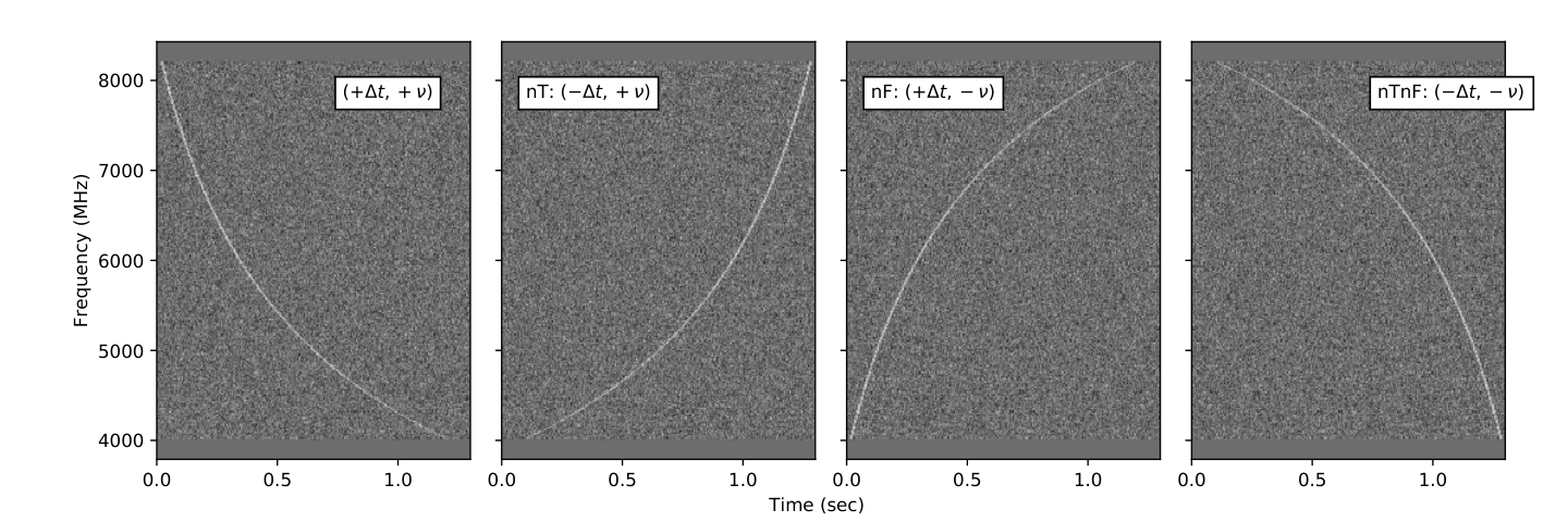
In order to search these four types of broadband transient signals (shown in Figure 8), we have deployed a state-of-the-art GPU-accelerated and ML-assisted broadband signal detection pipeline named SPANDAK. This pipeline is an extension of the pipeline used for the detection of – so far the only highest radio frequency – bursts from FRB (Gajjar et al. 2018). More details about the SPANDAK pipeline will be discussed in future publications (Gajjar et al. 2021 in prep.). As mentioned in Section IV.3, we only carried out these transient searches for our GBT data since scattering and dispersion losses at lower frequencies render such searches less sensitive. Some of the search parameters for our GBT C-band transient search are listed in Table 6. For simplicity, natural DM candidates will be referred to as pDM (i.e. positive DM) candidates and three other types of transient signals – nT, nF, and nTnF – will collectively be referred to as artificial DM (i.e. aDM) candidates for the remainder of the discussion.

V.2.1 Positive DM signal searches
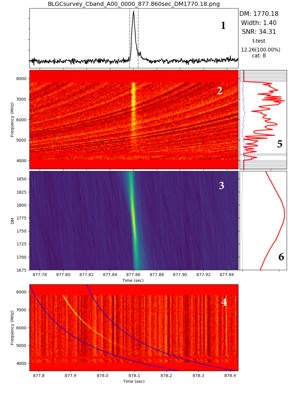
The GC region is likely to harbor an FRB-like magnetar population as suggested in Section II.4.3. We searched for such transients using SPANDAK with the parameters listed in Table 6 on the mid-temporal resolution data product mentioned in Table 4. We first collated 2 nearby frequency channels and reduced the frequency resolution by a factor of 2 to get 6656 channels as SPANDAK has a limitation of processing only up to 8k channels. We searched up to a DM of 5000 pc cm-3. With our final temporal and frequency resolution products, the maximum channel smearing we will get for the highest DM is ms. This is slightly higher than our sampling time of the data products (0.349 ms) used for this analysis. With this lower bound on the possible widths, we searched for bursts with widths up to 90 ms as mentioned in Table 6. We found a total 4467 pDM candidates from all the pointings shown in Figure 3. A summary of number of candidates observed from each of our C-band pointings are listed in Table 7. For each of the off-GC pointings (B and C rings) we roughly observed 80 to 100 candidates which is consistent with our lower S/Nmin threshold and interference environment. As can also be seen from Table 7, around 70% of the total candidates were found toward the GC(0,0) region. Figure 9 shows an example output plot from the SPANDAK pipeline. We visually inspected such plots for 4467 candidates and separated 667 candidates for further inspection. Figures 10a and 10b show the distribution of all observed candidates from one of the 30-min scans and the distribution of 667 candidates from our entire observations with a first visual inspection cut. Out of these candidates, we identified 603 candidates from the Galactic center magnetar, SGR J1745-2900, as is clearly evident from Figure 10b with a large fraction of these candidates around the DM of 1778 pc cm-3. The rest of the 63 candidates were viewed carefully by changing the number of sub-bands, number of time bins, and adjusting the detected DM to verify if the detected signal was real. Figure 11a shows one such example of an interesting candidate which was later rejected. After this careful inspection, we were unable to verify the validity of these 63 remaining candidates and were unable to find any new pDM transient signals from our observations originating from astrophysical processes.


V.2.2 Artificial DM signal searches
The interstellar medium heavily impacts any signal being transmitted close to the GC. We refer to the Galactic density model from Yao et al. 2017, and considered that the largest DM one is likely to encounter towards the GC is on the order of 4000 pc cm-3. It should be noted that density model by Yao et al. 2017 may sometimes over-predict the DM in the plane of the Galaxy. Another Galactic density model by Cordes & Lazio 2002 (NE2001) may be more accurate; however, towards the GC, it also predicts a similar high DM. All three types of aDM signals get impacted differently. For example, signals with nT-aDM are indistinguishable from naturally dispersed signals if they are transmitted originally with the aDM less than the DM contribution from the Galaxy. Hence, when we refer to the DM limit for these signals, original transmitted aDM would likely be pc cm-3. For nF-aDM and nTnF-DM types of signals, the dispersion due to interstellar medium heavily impacts their shape and would render them indistinguishable from interference. Thus, in order to recover their original aDM shape, we dedisperse all mid-time resolution data products at the DM of 4000 pc cm-3 before searching for nF-aDM and nTnF-aDM bursts. With this dispersion, we had to collate frequency resolution by a factor of 4 (3k channels) compared to the original mid-temporal resolution products. Thus, due to further channel smearing, our minimum burst width will be on the order of 0.7 ms for artificial transients across 4 to 8 GHz.
For the aDM signal searches, we searched twice the maximum pulse widths compared to our pDM search as indicated in Table 6. We found a total 2276 candidates combined from all three different aDM types with a S/Nmin cut of 10. Table 7 summarizes a number of candidates found from each of the pointings. Figure 10b shows a histogram of these candidates. From our initial inspection of SPANDAK plots (such as shown in Figure 9), we found 56 candidates for further inspection. Figure 11b and 11c show examples of two such interesting aDM candidates. Further discussion on these candidates are outlined in Section VI.1.
| Parkes: 1.0 to 4.0 GHz | |||||||||
| Pair | ON-source | RA | DEC | l | b | f2 | f3 | ||
| pointing | (h:m:s) | (d:m:s) | (deg) | (deg) | Events | Events | |||
| A1-B1 | A1 | 17:45:40.04 | -29:00:28.10 | 359.94 | -0.05 | 291 | 0 | ||
| B1 | 17:42:34.15 | -28:35:25.90 | 359.94 | 0.75 | 9,301 | 138 | |||
| A2-B2 | A2 | 17:45:18.09 | -29:08:19.17 | 359.79 | -0.05 | 1,424 | 0 | ||
| B2 | 17:42:12.06 | -28:43:15.04 | 359.79 | 0.75 | 7,149 | 36 | |||
| A3-B3 | A3 | 17:46:01.93 | -28:52:36.81 | 0.10 | -0.05 | 1,012 | 3 | ||
| B3 | 17:42:56.19 | -28:27:36.52 | 0.10 | 0.75 | 3,446 | 27 | |||
| A4-B4 | A4 | 17:46:00.21 | -29:08:32.63 | 359.87 | -0.18 | 1,116 | 0 | ||
| B4 | 17:42:54.00 | -28:43:32.13 | 359.87 | 0.62 | 3,384 | 15 | |||
| A5-B5 | A5 | 17:46:22.11 | -29:00:41.14 | 0.02 | -0.18 | 1,036 | 0 | ||
| B5 | 17:43:16.04 | -28:35:42.55 | 0.02 | 0.62 | 4,935 | 12 | |||
| A6-B6 | B6 | 17:44:57.98 | -29:00:14.25 | 359.87 | 0.09 | 786 | 0 | ||
| B6 | 17:41:52.26 | -28:35:08.43 | 359.87 | 0.88 | 2,436 | 9 | |||
| A7-B7 | A7 | 17:45:19.92 | -28:52:23.38 | 0.02 | 0.09 | 802 | 0 | ||
| B7 | 17:42:14.35 | -28:27:19.50 | 0.02 | 0.88 | 4,727 | 9 | |||
| GBT: 3.9 to 8 GHz | |||||||||
| Pair | ON-source | RA | DEC | l | b | f2 | f3 | pDM | aDM |
| pointing | (h:m:s) | (d:m:s) | (deg) | (deg) | Events | Events | Candidates | Candidates | |
| A00-C01 | A00 | 17:45:40.04 | -29:00:28.10 | 359.944 | -0.046 | 2 | 0 | see below | see below |
| C01 | 17:45:51.95 | -28:56:11.99 | 0.028 | -0.046 | 3,129 | 3 | 43 | 21 | |
| C07-A00 | C | 17:45:28.12 | -29:04:44.14 | 359.861 | -0.046 | 1,687 | 0 | 51 | 29 |
| A | 17:45:40.04 | -29:00:28.10 | 359.944 | -0.046 | 1 | 0 | see below | see below | |
| B01-B04 | B01 | 17:45:45.99 | -28:58:20.05 | 359.986 | -0.046 | 1 | 0 | 52 | 112 |
| B04 | 17:45:34.08 | -29:02:36.13 | 359.906 | -0.046 | 203 | 0 | 80 | 150 | |
| B02-B05 | B02 | 17:45:34.57 | -28:58:16.40 | 359.965 | -0.010 | 75 | 0 | 113 | 240 |
| B05 | 17:45:45.52 | -29:02:39.78 | 359.923 | -0.082 | 53 | 0 | 84 | 140 | |
| B03-B06 | B03 | 17:45:28.61 | -29:00:24.42 | 359.923 | -0.010 | 64 | 0 | 83 | 90 |
| B06 | 17:45:51.47 | -29:00:31.72 | 359.965 | -0.082 | 38 | 0 | 80 | 100 | |
| C02-C04 | C02 | 17:45:40.52 | -28:56:08.37 | 0.007 | -0.010 | 271 | 0 | 73 | 55 |
| C04 | 17:45:23.14 | -28:58:12.69 | 359.944 | 0.026 | 457 | 0 | 35 | 58 | |
| C03-C05 | C03 | 17:45:29.10 | -28:56:04.69 | 359.986 | 0.026 | 291 | 0 | 100 | 65 |
| C05 | 17:45:17.18 | -29:00:20.67 | 359.903 | 0.026 | 2,038 | 0 | 86 | 27 | |
| C08-C06 | C08 | 17:45:39.56 | -29:04:47.83 | 359.882 | -0.082 | 57 | 0 | 73 | 15 |
| C06 | 17:45:22.65 | -29:02:32.42 | 359.882 | -0.010 | 582 | 0 | 53 | 31 | |
| C11-C09 | C11 | 17:46:02.90 | -29:00:35.29 | 359.986 | -0.118 | 1,605 | 0 | 51 | 23 |
| C09 | 17:45:51.00 | -29:04:51.46 | 359.903 | -0.118 | 118 | 0 | 46 | 81 | |
| C10-C12 | C | 17:45:56.95 | -29:02:43.38 | 359.944 | -0.118 | 282 | 16 | 51 | 20 |
| C | 17:45:57.42 | -28:58:23.65 | 0.007 | -0.082 | 917 | 0 | 109 | 59 | |
| Deep | A | 17:45:40.04 | -29:00:28.10 | 359.944 | -0.046 | - | - | ||
VI Discussion
VI.1 Candidate signals from ETI
We carried out searches for two different types of beacons which are likely to originate from (a) a transmitter placed near the GC illuminating the entire Galaxy and/or (b) any star in the lines-of-sight of our pointings towards the GC.
VI.1.1 Narrowband drifting candidates
As mentioned earlier, we carried out three pairs of ON-OFF observations and compared narrowband drifting signals across ON and OFF pointings for all pairs. Some straightforward examples of candidates classified as RFI can be seen in Figure 7. A clear RFI signal can be seen in Figures 7a - 7c, where we see the signal appearing in all six observations. In these three examples, a clear and sometimes intermittent triplet pattern (central carrier with two side-bands) can be seen which is likely to be a terrestrial communication signal. If the drift rate of this signal was significantly non-zero and was not present in the off scans, this would be an incredibly intriguing signal. Signals shown in Figures 7a and 7c also appear to have similar frequency (4199.5 MHz) despite coming from different pointings. A slightly dimmer RFI signal can also be seen in Figure 7d for ON and OFF observations. Such weaker signals are less likely to be detected above our S/Nmin threshold and likely to be rejected automatically without careful visual inspection. Examples shown in Figures 7e and 7f are interesting candidates where a signal is seen in one and two ON-source pointings, respectively. However, upon careful inspection it can be seen that the same signal is also visible at the beginning of the OFF pointing. Additionally, the drift rate of these signals are close to zero and thus, they are likely to originate from terrestrial sources.
Although most of the examples shown in Figure 7 were detected with the GBT data, an interesting example was found in the A2-B2 (359.79-0.05 & 359.79+0.75) pair with the Parkes UWL observations. Figure 7g shows several closely spaced strong narrowband drifting signals in the , , and panels. This strong signal appears as a candidate event several times throughout our candidate list, both using filter 2 and 3 across a few other pointings. Since this is an interesting candidate passing our final filter 3, we carefully compared the detected frequency of the candidate against the satellite database and their transmission frequencies. Indeed, we find that the frequency at which these signals are found (1381 MHz) is also the frequency at which the GPS satellite Navstar transmits. Thus, due to its detection across other pointings and association of the detection frequency with a known satellite transmission, we are unable to consider this as a likely candidate of extra-terrestrial origin. Nevertheless, it is a good depiction of what we expect a potential ETI signal to look like: non-zero drifting and appearing in all 3 ON-observations but none of the OFF. The two remaining events from Figure 7: 7h and 7i are the most interesting. The candidate shown in Figure 7h is found at 4.197 GHz where a large concentration of hits are seen across other pointings as shown in Figure 5a and thus can still be rejected as RFI. However, the candidate shown in Figure 7i occurring at 6.408 GHz is unique and is seen only once in our entire set of observations (see Figure 5a). Since we did not find it to repeat during the other ON pointings, we still discard it as RFI due to some intermittent terrestrial source or coincidental passing of a low earth orbit satellite across our beam during that single 5-min observation pointing towards C09. In summary, we did not find any strong evidence of narrowband drifting signals based on our criteria. Thus, we can reject the presence of strong beacons transmitting between 1 to 8 GHz with a 100% duty cycle located either at the GC or from other line-of-sight stars. However, we should point out that there are a few caveats on these constraints we obtained on the existence of such signals. For example, we only searched a small fraction of drift-rate parameter space (4 Hz/sec) and with a reduced sensitivity towards higher drift rate (see Margot et al. 2021). Also, our detection pipeline may have an imperfect recovery rate and we might miss a strong signal in our data. We will address completeness of analysis pipeline in future publications (Perez et al. 2021 in prep).
VI.1.2 Broadband candidates
We carried out a search for three different types of aDM candidates for the first time. After eliminating candidates originating due to RFI, we shortlisted 56 candidates. We carefully further inspected these selected candidates by changing the number of frequency channels, number of bins, and adjusting aDM. Most of these candidates appear to occur due to peculiar interference which aligns so as to mimic the aDM dispersion pattern. For example, in Figure 11b, there is a comb of interference present between 4.2 to 4.4 GHz. These comb of narrow frequency interference coincidentally happen to align with the nT-aDM dispersion curve. Figure 11c shows another example of a nF-aDM candidate found towards the A00 field at the aDM of -1814 pc cm-3. This candidate is likely due to interference at zero DM, which due to its limited spectral coverage, appears to partially follow the nF dispersion curve. Overall, we did not find any real artificially dispersed candidates originating from a likely transmitter placed at the GC or from stars close to the GC. Since we only dedisperse the data products to a DM of 4000 pc cm-3 to compensate for their likely origin at the GC, with our current analysis we are unable to verify the existence of such signals transmitted from other stars along the line-of-sight towards the GC. In the future, we plan to dedisperse our data products at multiple DMs before searching aDM signals to compensate for their Galactic dispersion and likely origin from line-of-sight stars spread across 8.2 kpc.
VI.2 Number of stars surveyed
In Section II, we highlighted that a line-of-sight towards the GC encounters the largest number of habitable stars compared to any other direction in the sky. In this section, we make an order-of-magnitude estimation on the number of stars surveyed based on the stellar number density (stars/pc3) in the radial direction of our survey. Gowanlock et al. 2011 outlined various stellar number density models and found that the Carroll & Ostlie 2007 estimation of the number density profile appears to match the observed stellar density in the Solar neighbourhood. This number density is represented as a function of radial distance from the GC, R, and vertical height from the Galactic midplane, , as,
| (3) |
Here, n0 is the normalization factor which we consider from Gowanlock et al. 2011 as 5.502 stars/pc3. The constants Zthin=350 pc, Zthick=1000 pc, and hR=2.25 kpc are thin disk scale height, thick disk scale height, and radial scale, respectively. As can be seen, although stellar density falls off very quickly in the direction, for smaller angular scales, it can be considered to have constant stellar density. For example, at the distance of 8.5 kpc with our survey region of , the diameter of the region probed would be around 10 pc, for which the number density reduces by only 2.5% (from 5.96 to 5.81 stars/pc3). This is not a significant change; thus, we use the midplane density and take it as a constant for the scale height.
To calculate the total number of stars, we considered a cone in the Galactic midplane towards the GC with the Sun at the apex. The angle of the cone changes as a function of our observing frequencies and proposed target region. We considered stars up to the distance of 8.5 kpc from Earth which includes the central Galactic bulge which has the largest concentration of stars. For our current region, if we count the number of stars from Earth to the GC, we will encounter total stars. This number will decrease as we go to higher-frequencies with the GBT due to our reduced survey regions (see Table 2). For our already conducted survey of the Parkes region which covers two fields (see Figure 2), we estimated that we surveyed around 60 million stars. The large concentration of these total surveyed stars are likely to reside close to the GC region. As indicated in Figure 1, a large fraction of these stars, especially the ones that are closest to the GC, may host habitable planets and thus our survey provides some of the best constraints on the two types of beacons from the large number of habitable systems. We should highlight that these are only an order-of-magnitude estimates and gauging the exact numbers, especially for Parkes (), is a non-trivial task due to the validity of our assumed stellar number density model and small angle approximations.
VI.3 Survey sensitivity
We have conducted searches for two different signal types, and limits can be placed on our detection sensitivity to both these signal types. For narrowband drifting signals, the minimum detectable flux can be given as,
| (4) |
Here, Ssys is the system equivalent flux density, represents integration time, np is the number of polarizations, and are bandwidths of transmitted and received narrowband signals, respectively. For our survey we assumed a transmitted bandwidth of 1 Hz77 7 Interstellar scattering causes broadening of a narrow spectral line (Cordes & Lazio 1991). For transmitters near the Sun the broadening is Hz and thus unimportant but the strong scattering toward the GC can make this a significant effect. Thus, it is likely that transmitter bandwidth will be larger which will increase our sensitivity but for simplicity we have assumed it to be 1 Hz.. S/Nmin represents a desired threshold and is the dechirping efficiency. As mentioned in Section V.1, due to our frequency ( Hz) and temporal (18 sec) resolutions, high drift rate signals get spread across multiple channels which reduces our sensitivity. This dechirping efficiency can also be expressed as follows for our survey.
| (5) |
Here, is the trial drift rate under consideration. Our dechirping efficiency reaches its maximum for drift rates 0.16 Hz/sec and gradually declines beyond this limit. As mentioned in Section V.1, future narrowband searches will improve this efficiency by collapsing nearby channels or by using a moving boxcar of corresponding width for the number of channels a given signal is likely to have spread across (Price et al. 2020).
For the broadband pDM and aDM transient signals, the minimum detectable flux can be expressed as,
| (6) |
Here, is the pulse width of pDM and aDM candidates, is the total instantaneous bandwidth, and is the loss due to digitization. For pDM candidates we used a S/Nmin threshold of 6 and for aDM candidates we used a S/Nmin threshold of 10. For simplicity, we considered scatter-independent pulse widths. A more accurate width estimation based on the scatter broadening and corresponding sensitivity limitation are discussed further in Section VI.6. For both the signal types (narrowband and broadband), the Ssys can also be represented as,
| (7) |
Here, Tsys is the system temperature at typical weather conditions88 8 Table 2.2 in https://science.nrao.edu/facilities/gbt/observing/GBTog.pdf, is the Boltzmann constant, and Aeff is the effective aperture of the receiving antenna. The GC region contains a significant amount of background flux, especially with the lower frequency receivers (up to Ku-band). The excess noise contribution, which is expressed as TGC, will make a significant additional contribution to the Ssys (Johnston et al. 2006; Macquart et al. 2010), and need to be included in the sensitivity calculations. Law et al. 2008 conducted a detailed continuum survey of the GC region using the GBT and computed a calibrated map of the region. Rajwade et al. 2017. used these measurements and derived the frequency dependence of this excess noise from the GC as,
| (8) |
Here, is the observing frequency. As it can be seen, this will add a huge contribution to the system temperature at lower frequencies. For example, at 0.7 GHz from the UWL at Parkes, the expected noise contribution from the GC would be of the order of 800 K. Considering this contribution, our survey sensitivity is listed in Figure 12 for both narrow and broadband signals. As it can be seen, Ku and KFPA bands provide maximum sensitivity for both types of signals with contribution from the GC dominating at lower frequency, and contribution from the Earth’s atmosphere dominating the Tsys at higher frequencies. Based on our minimum Smin,narrow and Smin,broad at various frequencies, we can calculate the corresponding Equivalent Isotropic Radiated Power (EIRP) at all our observing bands as,
| (9) |
For transmitters at the distance of the GC, the minimum EIRPGC are shown in Figure 12. It is evident that the minimum EIRP sensitivities of W and W/Hz are possible to achieve at the KFPA band for the narrowband and broadband transient signals, respectively. For our current survey with the GBT C-band and Parkes-UWL, we estimate minimum EIRP detection sensitivity of around W ( 1019 W for the signals with highest drift rates) and W ( 1020 W for the signals with highest drift rates) for the narrowband drifting signals, respectively. Similarly, for the broadband artificially dispersed signals from GBT C-band survey, we estimate a minimum detectable EIRP of the order of W/Hz. It is clearly evident that broadband signal allows much better sensitivity to provide better constraints on the weaker signals if they are band limited. However, since such signals are assumed to last for only a fraction of a second, we rely upon the repeatability of such signals which is further discussed in Section VI.5.
VI.4 Survey figure of merit
There have been several SETI surveys that have been conducted in the past six decades (Enriquez et al. 2017; Wright et al. 2018, and references therein). These surveys have primarily searched for narrowband drifting signals and thus they can be compared with each other based on the total number of stars they surveyed (or total area of the sky covered), total bandwidth utilized, detection sensitivity and other such parameters. For narrowband signals, the Drake figure-of-merit (DFM; Drake et al. 1984) has been computed by many previous SETI surveys and can be expressed as,
| (10) |
where is the area of the sky surveyed, is the minimum detectable flux average across all observing frequencies, and is the total observing bandwidth. For our survey with the GBT across 3.9 – 8 GHz, we found the DFM to be for the narrowband signals with drift-rates 0.16 Hz/sec and for the highest drift-rate considered for our survey. It should be noted that the DFM has a number of limitations as outlined by Enriquez et al. 2017 and Margot et al. 2021. For example, the DFM does not consider a range of drift-rates and dechirping efficiency which heavily impacts Smin,avg for a survey under consideration (Margot et al. 2021). Moreover, the DFM assumes a uniform distribution of ETI transmitters. For surveys like ours, where a large concentration of stars are likely to reside within our beam towards the GC, the DFM does not provide an accurate comparison. A better figure-of-merit is the Continuous Waveform Transmitter Rate (CWTFM), as introduced by Enriquez et al. 2017, which is also for narrowband signals and can be given as,
| (11) |
Here, is the fractional bandwidth , is the normalization factor such that CWTFM = 1 when the EIRP is equivalent to the EIRP of the Arecibo radio telescope’s planetary radar ( W), = 0.5, and Nstars = 1000. For our conducted survey, as discussed in Section VI.2, we can estimated the number of stars using the stellar density model and estimate the corresponding EIRP limits (see Section VI.3). We found that for the UWL and C-band, we surveyed around 60 million and 0.6 million stars, respectively. Figure 13 shows the measured CWTFM for our current C-band and UWL surveys compared with some of the prominent SETI surveys reported earlier. It is clearly evident that with our current survey, we are already able to push the limit of transmitter-rate slope lower than what was obtained from previous SETI surveys. By extending this survey to other frequencies from the GBT and covering all the pointings from the Parkes telescopes, we are likely to push the CWFTM slope much lower and able to constrain the presence of technosignatures across a wide range of frequencies. Furthermore, Figure 12a shows a comparison of sensitivity of narrowband signals of our survey with some of the prominent SETI surveys. As it is clearly evident, no other survey has ever explored the frequency coverage we aim to search with our survey. Moreover, these comparisons are only carried out for narrowband drifting signals. Our survey is already the only survey to search for artificially dispersed signals which have never been explored and thus cannot be compared with any previous SETI surveys.
VI.5 Limits on repeatability of broadband signals from ETIs

We searched for three different types of artificially-dispersed broadband transient bursts likely to originate from deliberately transmitted ETI beacons. In future work, we will provide a detailed discussion on harmonic searches for these broadband signals. In this section, we evaluate the repetition rate of these broadband bursts from our GC deep observations. Figure 14 shows one of the scenarios of repeating broadband signals originating from a rotating beam from an artificial beacon99 9 Here, we are only considering rotation of an artificial beam transmitting pulses with aDM dispersion to illuminate the Galaxy. We are not considering sweeping of such an artificial beam to produce aDM bursts such as in the case of pulsars generating pDM bursts. Thus, we are not constrained by the beaming fraction of such a beam.. We can also infer different mechanisms which do not necessarily require a rotating beam but can still generate repeated bursts of similar nature. Such rotating beams of an artificial nature have been proposed earlier. For example, Benford et al. 2010a suggested such a beacon situated at the GC would be the most energy-efficient way to signal the entire Galaxy. Shostak & Tarter 1985 have also considered narrowband signals originating from such a rotating beacon. We did not find any strong aDM candidates; thus, considering length and separation between all our observations, we can reject repetition of all three types of broadband signals. Table 3 lists all the observing dates and lengths of each of these observations. We arranged them on the time-axis and then simulated pulse trains with a range of periods. We also adjusted the phase (or offset) of these bursts within the corresponding period under consideration. For each period, we calculated the number of instances of offset phases which would have allowed us to see at least one pulse. Here, we assumed that we are likely to detect a burst at every period. Figure 14 shows the probability of rejecting periods for such bursts. We can reject any mechanism which can regularly produce pulses across 3.9 to 8 GHz with the repetition period of around 4.3 hours with high accuracy (considering imperfect recovery rate of our search pipeline). For larger repetition periods up to 10 hours, we can reject such mechanism with 50% probability while for further large periods up to 100 hours, rejection probability is marginal (10%) from our observations. In the future, we plan to extend this analysis for narrowband signals and will also schedule our observations such as to allow sufficient epoch sampling to reject larger repeating periodicity with better significance. These limits are non-trivial to apply to astrophysical sources such as magnetars which are not known to produce strong transient pulses during every rotation and their beam of emission not necessarily likely to reside in the plane as we assumed for this analysis.
VI.6 SGR J1745–2900 and constraints on other transients from magnetars near the GC
We detected 603 single pulses from SGR J1745–2900 across 3.9 to 8.0 GHz with a total of 6.6 h of observations. These single pulses exhibit a wide variety of pulse shapes with single and multiple components. Figure 15 shows examples of four different types of single pulses seen from SGR J1745–2900 from our observations: a narrow single pulse with a scattering tail, a pulse with unresolved multiple-components, and two well resolved dual-component pulses. This is consistent with single pulses seen around similar frequencies by Pearlman et al. 2018 and Wharton et al. 2019. A detailed spectro-temporal analysis of these bursts is beyond the scope of this paper and will be reported in future publications. These observations are useful to constrain the presence of other radio magnetars at the GC producing transient bursts.

Scattering due to a relatively dense environment near the GC likely limits the detection of other transients. In order to estimate scatter-broadened pulse widths at our observed frequencies, we utilized a narrow single peaked pulse from SGR J1745–2900 shown in Figure 15 for further analysis. Spitler et al. 2014 estimated that the scatter broadening () from SGR J1745–2900 is of the order of sec at 1 GHz with a spectral index of . Considering a similar spectral index, the expected will be ms at 6 GHz. Measuring the observed is challenging, as suggested by Krishnakumar et al. 2017, due to the degeneracy of the unknown intrinsic pulse width and unresolved emission components. To model our underlying observed single pulse, we assumed a simple intrinsic single pulse with a Gaussian profile from the source, convolved with the for transmission through the ISM; where is a step function with for and for . For the intrinsic pulse, we considered a pulse width of 1.8 ms reported from Pearlman et al. 2018 at 8.4 GHz, which is close to the highest end of our observed band. Similar techniques have been used by Krishnakumar et al. 2017 and Krishnakumar et al. 2019 to estimate . We found the ms by fitting this model to the narrow pulse shown in Figure 15. This is slightly higher and not consistent with the spectral index of reported earlier at lower frequencies by Spitler et al. 2014. Similar inconsistencies were also reported by Pearlman et al. 2018. It is also likely that the larger scatter broadening is due to an unresolved emission component at the trailing edge of the pulse.
The scatter broadening time scale found from the narrow SGR J1745–2900 burst can be utilized to place a limit on other FRB-like Galactic magnetars and millisecond pulsar (MSP) located in a similar environment around the GC. We reevaluated our minimum detection limit for the broadband signals calculated in Section VI.3. We find that for our current survey across 3.9 to 8 GHz for transients, we were sensitive to bursts with peak flux density of around 68 mJy which is equivalent to the peak luminosity of erg s-1 across our band for a source located at the GC. Although average flux densities of folded profiles of radio-loud magnetars are relatively lower, single pulses from them do exhibit bright emission. For example, XTE J1810–197, a known Galactic radio magnetar, was seen to produce bright transient radio pulses up to 42 GHz (Camilo et al. 2006). XTE J1810–197 showed many single pulses with a peak flux of Jy at 6.4 GHz which corresponds to a peak luminosity of around erg s-1 across their 500 MHz band. Similarly, another radio-loud magnetar, PSR J1622–4950, is known to show bursts with a peak flux of around 16 Jy (Levin et al. 2010b), which corresponds to a peak luminosity of erg s-1. This is an order of magnitude larger than our limit. Moreover, the recently detected FRB-like Galactic magnetar, SGR 1935+2154, also exhibits a bright luminosity on the order of erg s-1 (The CHIME/FRB Collaboration et al. 2020) which is several orders of magnitude larger than our peak luminosity limit. Since our longest observing run was about 4.3 h (see Table 3), we can reject the presence of any transient signal with a typical burst-rate of bursts h-1 at our radio luminosity limit. A few of the radio magnetars are known to produce transient radio bursts with much larger burst rates. For example, SGR J1745–2900 produced bursts hr-1 as measured from our observations.
Our scatter-broadened limits are also important as many different theories have been proposed to solve the missing pulsar problem. For example, the GC has been considered to favor MSP production (Bartels et al. 2016). As we found a scatter broadening timescale of ms, any MSP signals with much smaller intrinsic pulse widths than normal pulsars are likely to get scattered and will therefore be undetectable up to our highest frequency of 8 GHz. Extension of our survey to higher frequencies would be ideal to search for other such MSPs near the GC.
VII Conclusion
In this paper, by extending the habitability model of Gowanlock et al. 2011 to the inner 2.5 kpc region, we demonstrated that a line-of-sight towards the GC is likely to render the largest concentration and highest number density of habitable worlds. The GC region also provides an ideal Schelling point for advanced civilizations to place a powerful transmitter to efficiently send beacons across the entire Milky Way. Thus, the GC is one of the primary targets of the BL program (Isaacson et al. 2017). We outlined our survey strategy for the most comprehensive search for evidence of intelligent life ever conducted by utilizing a large fraction of the accessible radio window (0.7 to 93 GHz) from the GBT and Parkes telescopes. We compared the sensitivity of our survey to some of the prominent SETI surveys and demonstrate that our survey has remarkable sensitivity with a frequency span never before explored for SETI.
We have reported early results from our survey of the GC region across 1 to 8 GHz with around 11.2 and 7 h of observations from the GBT and Parkes telescopes, respectively. We carried out searches for standard narrowband drifting signals, along with, for the first time, three different types of broadband artificially-dispersed transient signals (up to a DM of –5000 pc cm-3) using our state-of-the-art GPU accelerated tools. We did not find a strong beacon signal for any of these signal categories searched. However, our survey already placed a constraint on the existence of narrowband transmitters of in 60 million stars toward the GC across 1 to 4 GHz with EIRP W (and W for the highest drift-rate signals). We were also able to place meaningful constraints for the first time on the existence of narrowband and broadband transmitters in in half a million stars across 3.9 to 8 GHz with EIRP W (and W for the highest drift-rate signals) and W/Hz, respectively. With our deep targeted observations of the GC, we were also able to reject the existence of periodic broadband beacons showing characteristic aDM dispersion pattern with periods h with similar EIRPs.
We also searched for astrophysical transient signals from other radio-loud magnetars near the GC. We searched for broadband pulses up to a DM of 5000 pc cm-3 with pulse widths ranging from 0.3 to 90 ms with S/Nmin . We found 603 single pulses from SGR J1745–2900 and we determined a scatter broadening on the order of 4 ms from one of the narrow detected pulses. Based on the scatter broadening timescale, we ruled out the likely existence of other transient sources with a luminosity limit of erg s-1 with a burst-rate of burst hr-1. This is around the typical peak luminosity of other Galactic radio-loud magnetars.
VIII Acknowledgments
We would like to thank the anonymous referee for a critical review of the paper and for suggesting several improvements to the manuscript. Breakthrough Listen is managed by the Breakthrough Initiatives, sponsored by the Breakthrough Prize Foundation. SC, JMC, and AS acknowledge support from the National Science Foundation (AAG 1815242). VG thanks Alex Pettitt for giving us permission to use a sketch of the milky-way. The Parkes radio telescope is part of the Australia Telescope National Facility which is funded by the Australian Government for operation as a National Facility managed by CSIRO. The Green Bank Observatory is a facility of the National Science Foundation, operated under cooperative agreement by Associated Universities, Inc. We thank the staff at Parkes and Green Bank observatories for their operational support. We thank all the frontline workers during this global pandemic and all the California firefighters for keeping most of us out of harm’s way.
References
- Backus & Project Phoenix Team (2004) Backus, P. R., & Project Phoenix Team. 2004, in Bulletin of the American Astronomical Society, Vol. 36, American Astronomical Society Meeting Abstracts #204, 805
- Bartels et al. (2016) Bartels, R., Krishnamurthy, S., & Weniger, C. 2016, Phys. Rev. Lett., 116, 051102, doi: 10.1103/PhysRevLett.116.051102
- Benford et al. (2010a) Benford, G., Benford, J., & Benford, D. 2010a, Astrobiology, 10, 491, doi: 10.1089/ast.2009.0394
- Benford et al. (2010b) Benford, J., Benford, G., & Benford, D. 2010b, Astrobiology, 10, 475, doi: 10.1089/ast.2009.0393
- Bochenek et al. (2020) Bochenek, C. D., Ravi, V., Belov, K. V., et al. 2020, arXiv e-prints, arXiv:2005.10828. https://arxiv.org/abs/2005.10828
- Bower et al. (2014) Bower, G. C., Deller, A., Demorest, P., et al. 2014, The Astrophysical Journal Letters, 780, L2. http://stacks.iop.org/2041-8205/780/i=1/a=L2
- Bryson et al. (2021) Bryson, S., Kunimoto, M., Kopparapu, R. K., et al. 2021, AJ, 161, 36, doi: 10.3847/1538-3881/abc418
- Brzycki et al. (2020) Brzycki, B., Siemion, A. P. V., Croft, S., et al. 2020, arXiv e-prints, arXiv:2006.04362. https://arxiv.org/abs/2006.04362
- Camilo et al. (2006) Camilo, F., Ransom, S. M., Halpern, J. P., et al. 2006, Nature, 442, 892, doi: 10.1038/nature04986
- Camilo et al. (2007) Camilo, F., Ransom, S. M., Peñalver, J., et al. 2007, The Astrophysical Journal, 669, 561, doi: 10.1086/521548
- Carroll & Ostlie (2007) Carroll, B. W., & Ostlie, D. A. 2007, An Introduction to Modern Astrophysics, 2nd edn., ed. S. F. P. Addison-Wesley
- Carroll-Nellenback et al. (2019) Carroll-Nellenback, J., Frank, A., Wright, J., & Scharf, C. 2019, AJ, 158, 117, doi: 10.3847/1538-3881/ab31a3
- Cocconi & Morrison (1959) Cocconi, G., & Morrison, P. 1959, Nature, 184, 844, doi: 10.1038/184844a0
- Cole & Ekers (1979) Cole, T. W., & Ekers, R. D. 1979, Proceedings of the Astronomical Society of Australia, 3, 328
- Comisso & Asenjo (2021) Comisso, L., & Asenjo, F. A. 2021, Phys. Rev. D, 103, 023014, doi: 10.1103/PhysRevD.103.023014
- Cordes et al. (1997) Cordes, J. M., Lazio, J. W., & Sagan, C. 1997, ApJ, 487, 782, doi: 10.1086/304620
- Cordes & Lazio (1991) Cordes, J. M., & Lazio, T. J. 1991, The Astrophysical Journal, 376, 123, doi: 10.1086/170261
- Cordes & Lazio (1997) Cordes, J. M., & Lazio, T. J. W. 1997, ApJ, 475, 557, doi: 10.1086/303569
- Cordes & Lazio (2002) Cordes, J. M., & Lazio, T. J. W. 2002, arXiv: astro-ph/0207156
- Degenaar et al. (2013) Degenaar, N., Reynolds, M. T., Miller, J. M., Kennea, J. A., & Wijnands, R. 2013, The Astronomer’s Telegram, 5006, 1
- Deneva et al. (2009) Deneva, J. S., Cordes, J. M., & Lazio, T. J. W. 2009, The Astrophysical Journal Letters, 702, L177, doi: 10.1088/0004-637X/702/2/L177
- Dexter & O’Leary (2014) Dexter, J., & O’Leary, R. M. 2014, The Astrophysical Journal, 783, L7, doi: 10.1088/2041-8205/783/1/L7
- Di Stefano & Ray (2016) Di Stefano, R., & Ray, A. 2016, The Astrophysical Journal, 827, 54, doi: 10.3847/0004-637X/827/1/54
- Drake et al. (1984) Drake, F., Wolfe, J. H., & Seeger, C. L. 1984, SETI science working group report, 2244
- Dressing & Charbonneau (2015) Dressing, C. D., & Charbonneau, D. 2015, ApJ, 807, 45, doi: 10.1088/0004-637X/807/1/45
- Eatough et al. (2013a) Eatough, R., Karuppusamy, R., Kramer, M., et al. 2013a, The Astronomer’s Telegram, 5040
- Eatough et al. (2013b) Eatough, R. P., Falcke, H., Karuppusamy, R., et al. 2013b, Nature, 501, 391, doi: 10.1038/nature12499
- Enriquez et al. (2017) Enriquez, J. E., Siemion, A., Foster, G., et al. 2017, ApJ, 849, 104, doi: 10.3847/1538-4357/aa8d1b
- Gajjar et al. (2020) Gajjar, V., Perez, K., Siemion, A., et al. 2020, The Astronomer’s Telegram, 13575, 1
- Gajjar et al. (2018) Gajjar, V., Siemion, A. P. V., Price, D. C., et al. 2018, ApJ, 863, 2, doi: 10.3847/1538-4357/aad005
- Gajjar et al. (2019) Gajjar, V., Siemion, A., Croft, S., et al. 2019, in BAAS, Vol. 51, 223. https://arxiv.org/abs/1907.05519
- Genzel et al. (2010) Genzel, R., Eisenhauer, F., & Gillessen, S. 2010, Reviews of Modern Physics, 82, 3121, doi: 10.1103/RevModPhys.82.3121
- Ghez et al. (2008) Ghez, A. M., Salim, S., Weinberg, N. N., et al. 2008, ApJ, 689, 1044, doi: 10.1086/592738
- Gowanlock et al. (2011) Gowanlock, M. G., Patton, D. R., & McConnell, S. M. 2011, Astrobiology, 11, 855, doi: 10.1089/ast.2010.0555
- Gravity Collaboration et al. (2019) Gravity Collaboration, Abuter, R., Amorim, A., et al. 2019, A&A, 625, L10, doi: 10.1051/0004-6361/201935656
- Hankins & Eilek (2007) Hankins, T. H., & Eilek, J. A. 2007, The Astrophysical Journal, 670, 693, doi: 10.1086/522362
- Harp et al. (2012) Harp, G. R., Ackermann, R. F., Blair, S. K., et al. 2012, ArXiv e-prints. https://arxiv.org/abs/1211.6470
- Harp et al. (2016) Harp, G. R., Richards, J., Tarter, J. C., et al. 2016, The Astronomical Journal, 152, 181, doi: 10.3847/0004-6256/152/6/181
- Harp et al. (2018) Harp, G. R., Ackermann, R. F., Astorga, A., et al. 2018, ApJ, 869, 66, doi: 10.3847/1538-4357/aaeb98
- Hobbs et al. (2020) Hobbs, G., Manchester, R. N., Dunning, A., et al. 2020, PASA, 37, e012, doi: 10.1017/pasa.2020.2
- Horowitz & Sagan (1993) Horowitz, P., & Sagan, C. 1993, ApJ, 415, 218, doi: 10.1086/173157
- Howell et al. (2014) Howell, S. B., Sobeck, C., Haas, M., et al. 2014, PASP, 126, 398, doi: 10.1086/676406
- Isaacson et al. (2017) Isaacson, H., Siemion, A. P. V., Marcy, G. W., et al. 2017, Publications of the Astronomical Society of the Pacific, 129, 054501
- Isaacson et al. (2017) Isaacson, H., Siemion, A. P. V., Marcy, G. W., et al. 2017, PASP, 129, 054501, doi: 10.1088/1538-3873/aa5800
- Jiménez-Torres et al. (2013) Jiménez-Torres, J. J., Pichardo, B., Lake, G., & Segura, A. 2013, Astrobiology, 13, 491, doi: 10.1089/ast.2012.0842
- Johnston et al. (2006) Johnston, S., Kramer, M., Lorimer, D. R., et al. 2006, MNRAS, 373, L6, doi: 10.1111/j.1745-3933.2006.00232.x
- Kennea et al. (2013) Kennea, J. A., Krimm, H., Barthelmy, S., et al. 2013, The Astronomer’s Telegram, 5009, 1
- Krishnakumar et al. (2017) Krishnakumar, M. A., Joshi, B. C., & Manoharan, P. K. 2017, ApJ, 846, 104, doi: 10.3847/1538-4357/aa7af2
- Krishnakumar et al. (2019) Krishnakumar, M. A., Maan, Y., Joshi, B. C., & Manoharan, P. K. 2019, ApJ, 878, 130, doi: 10.3847/1538-4357/ab20c5
- Law et al. (2008) Law, C. J., Yusef‐Zadeh, F., Cotton, W. D., & Maddalena, R. J. 2008, The Astrophysical Journal Supplement Series, 177, 255–274, doi: 10.1086/533587
- Lebofsky et al. (2019) Lebofsky, M., Croft, S., Siemion, A. P. V., et al. 2019, PASP, 131, 124505, doi: 10.1088/1538-3873/ab3e82
- Levin et al. (2010a) Levin, L., Bailes, M., Bates, S., et al. 2010a, The Astrophysical Journal Letters, 721, L33, doi: 10.1088/2041-8205/721/1/L33
- Levin et al. (2010b) —. 2010b, ApJ, 721, L33, doi: 10.1088/2041-8205/721/1/L33
- Li et al. (2020) Li, D., Gajjar, V., Wang, P., et al. 2020, Research in Astronomy and Astrophysics, 20, 078, doi: 10.1088/1674-4527/20/5/78
- Lineweaver et al. (2004) Lineweaver, C. H., Fenner, Y., & Gibson, B. K. 2004, Science, 303, 59, doi: 10.1126/science.1092322
- Lipman et al. (2018) Lipman, D., Isaacson, H., Siemion, A. P. V., et al. 2018, arXiv.org
- Liu et al. (2012) Liu, K., Wex, N., Kramer, M., Cordes, J. M., & Lazio, T. J. W. 2012, ApJ, 747, 1, doi: 10.1088/0004-637X/747/1/1
- MacMahon et al. (2018) MacMahon, D. H. E., Price, D. C., Lebofsky, M., et al. 2018, PASP, 130, 044502, doi: 10.1088/1538-3873/aa80d2
- Macquart et al. (2010) Macquart, J.-P., Kanekar, N., Frail, D. A., & Ransom, S. M. 2010, The Astrophysical Journal, 715, 939, doi: 10.1088/0004-637X/715/2/939
- Margot et al. (2021) Margot, J.-L., Pinchuk, P., Geil, R., et al. 2021, AJ, 161, 55, doi: 10.3847/1538-3881/abcc77
- Mori et al. (2013) Mori, K., Gotthelf, E. V., Zhang, S., et al. 2013, The Astrophysical Journal Letters, 770, L23, doi: 10.1088/2041-8205/770/2/L23
- Morrison & Gowanlock (2015) Morrison, I. S., & Gowanlock, M. G. 2015, Astrobiology, 15, 683, doi: 10.1089/ast.2014.1192
- Newman & Sagan (1981) Newman, W. I., & Sagan, C. 1981, Icarus, 46, 293, doi: https://doi.org/10.1016/0019-1035(81)90135-4
- Oliver & Billingham (1971) Oliver, B. M., & Billingham, J., eds. 1971, Project Cyclops: A Design Study of a System for Detecting Extraterrestrial Intelligent Life (NASA)
- Pearlman et al. (2018) Pearlman, A. B., Majid, W. A., Prince, T. A., Kocz, J., & Horiuchi, S. 2018, ApJ, 866, 160, doi: 10.3847/1538-4357/aade4d
- Pettitt et al. (2015) Pettitt, A. R., Dobbs, C. L., Acreman, D. M., & Bate, M. R. 2015, MNRAS, 449, 3911, doi: 10.1093/mnras/stv600
- Pfahl & Loeb (2004) Pfahl, E., & Loeb, A. 2004, The Astrophysical Journal, 615, 253, doi: 10.1086/423975
- Pinchuk et al. (2019) Pinchuk, P., Margot, J.-L., Greenberg, A. H., et al. 2019, The Astronomical Journal, 157, 122, doi: 10.3847/1538-3881/ab0105
- Prestage et al. (2015) Prestage, R. M., Bloss, M., Brandt, J., et al. 2015, in 2015 URSI-USNC Radio Science Meeting, 4, doi: 10.1109/USNC-URSI.2015.7303578
- Price et al. (2018) Price, D. C., MacMahon, D. H. E., Lebofsky, M., et al. 2018, Publications of the Astronomical Society of Australia, 35, 213
- Price et al. (2020) Price, D. C., Enriquez, J. E., Brzycki, B., et al. 2020, AJ, 159, 86, doi: 10.3847/1538-3881/ab65f1
- Rajwade et al. (2017) Rajwade, K. M., Lorimer, D. R., & Anderson, L. D. 2017, Monthly Notices of the Royal Astronomical Society, 471, 730–739, doi: 10.1093/mnras/stx1661
- Schelling (1960) Schelling, C. T. 1960, The strategy of conflict (Oxford University Press)
- Sheikh et al. (2020) Sheikh, S. Z., Siemion, A., Enriquez, J. E., et al. 2020, The Astronomical Journal, 160, 29, doi: 10.3847/1538-3881/ab9361
- Sheikh et al. (2019) Sheikh, S. Z., Wright, J. T., Siemion, A., & Enriquez, J. E. 2019, The Astrophysical Journal, 884, 14, doi: 10.3847/1538-4357/ab3fa8
- Shostak & Tarter (1985) Shostak, G., & Tarter, J. 1985, Acta Astronautica, 12, 369 , doi: https://doi.org/10.1016/0094-5765(85)90071-2
- Siemion et al. (2010) Siemion, A., Korff, J. V., McMahon, P., et al. 2010, Acta Astronautica, 67, 1342. http://linkinghub.elsevier.com/retrieve/pii/S0094576510000299
- Siemion et al. (2013) Siemion, A. P. V., Demorest, P., Korpela, E., et al. 2013, The Astrophysical Journal, 767, 94, doi: 10.1088/0004-637X/767/1/94
- Spitler et al. (2014) Spitler, L. G., Lee, K. J., Eatough, R. P., et al. 2014, The Astrophysical Journal Letters, 780, L3, doi: 10.1088/2041-8205/780/1/L3
- Surnis et al. (2020a) Surnis, M., Joshi, B. C., Bagchi, M., et al. 2020a, The Astronomer’s Telegram, 13777, 1
- Surnis et al. (2020b) —. 2020b, The Astronomer’s Telegram, 13799, 1
- Tarter (2003) Tarter, J. 2003, Annual Reviews of Astronomy and Astrophysics, 39, 511. http://arjournals.annualreviews.org/doi/abs/10.1146/annurev.astro.39.1.511?prevSearch=%255Bauthor%253A%2Btarter%2Bjill%255D&searchHistoryKey=
- Tarter et al. (1980) Tarter, J., Cuzzi, J., Black, D., & Clark, T. 1980, Icarus, 42, 136, doi: 10.1016/0019-1035(80)90251-1
- The CHIME/FRB Collaboration et al. (2020) The CHIME/FRB Collaboration, :, Andersen, B. C., et al. 2020, arXiv e-prints, arXiv:2005.10324. https://arxiv.org/abs/2005.10324
- Tingay et al. (2016) Tingay, S. J., Tremblay, C., Walsh, A., & Urquhart, R. 2016, ApJ, 827, L22, doi: 10.3847/2041-8205/827/2/L22
- Tingay et al. (2018) Tingay, S. J., Tremblay, C. D., & Croft, S. 2018, ApJ, 856, 31, doi: 10.3847/1538-4357/aab363
- Torne et al. (2015) Torne, P., Eatough, R. P., Karuppusamy, R., et al. 2015, Monthly Notices of the Royal Astronomical Society: Letters, 451, L50, doi: 10.1093/mnrasl/slv063
- Valdes & Freitas (1986) Valdes, F., & Freitas, R. A., J. 1986, Icarus, 65, 152, doi: 10.1016/0019-1035(86)90069-2
- Verschuur (1973) Verschuur, G. L. 1973, Icarus, 19, 329, doi: 10.1016/0019-1035(73)90109-7
- von Korff (2010) von Korff, J. 2010, UC Berkeley PhD Thesis in Physics. http://seti.berkeley.edu/sites/default/files/vonkorff_thesis_full_051010.pdf
- Wharton et al. (2019) Wharton, R. S., Chatterjee, S., Cordes, J. M., et al. 2019, ApJ, 875, 143, doi: 10.3847/1538-4357/ab100a
- Worden et al. (2017) Worden, S. P., Drew, J., Siemion, A., et al. 2017, Acta Astronautica, 139, 98
- Wordsworth & Pierrehumbert (2014) Wordsworth, R., & Pierrehumbert, R. 2014, ApJ, 785, L20, doi: 10.1088/2041-8205/785/2/L20
- Wright (2018) Wright, J. T. 2018, Exoplanets and SETI, 186, doi: 10.1007/978-3-319-55333-7_186
- Wright et al. (2018) Wright, J. T., Kanodia, S., & Lubar, E. 2018, AJ, 156, 260, doi: 10.3847/1538-3881/aae099
- Yao et al. (2017) Yao, J. M., Manchester, R. N., & Wang, N. 2017, ApJ, 835, 29, doi: 10.3847/1538-4357/835/1/29
- Zhang et al. (2020) Zhang, C. F., Jiang, J. C., Men, Y. P., et al. 2020, The Astronomer’s Telegram, 13699, 1