Thermomagnetic modification of the anomalous magnetic moment of quarks using the NJL model

The influence of an external magnetic field on the vacuum structure of quantum chromodynamics (QCD) and its modifications at finite temperature and/or chemical potential can play an important role in many physical systems (see Ref. Kharzeev et al. 2013 for review). For example, it is conjectured by some cosmological models that during the electroweak phase transition in the early universe, extremely strong magnetic field as high as $\sim 10^{23}$ G might have been produced Vachaspati 1991; Campanelli 2013 (note that in natural units, $10^{18}{\rm\penalty\ G}\approx m_{\pi}^{2}\approx 0.02\penalty\ {\rm GeV}^{2}$). The magnetic field on the surface of certain compact stars called magnetars, is of the order of $\sim 10^{15}$ G, while in the interior it is estimated to reach about $\sim 10^{18}$ G Duncan and Thompson 1992; Thompson and Duncan 1993; Lai and Shapiro 1991. Most importantly, in non-central or asymmetric heavy-ion collisions (HICs) at RHIC and LHC, strong magnetic fields of the order of $\sim 10^{18}$ G Kharzeev et al. 2008; Skokov et al. 2009 or larger may be transiently generated. It is, however, predicted that the presence of a finite electrical conductivity of the hot and dense medium created during HICs can delay the decay of these time-dependent magnetic fields substantially Tuchin 2013; Gursoy et al. 2014; Tuchin 2016; Das et al. 2017. Thus, being comparable to the QCD scale i.e. $eB\approx m_{\pi}^{2}$, such high magnetic fields can influence substantial change in the deconfined medium of strongly interacting quarks and gluons known as the quark-gluon plasma (QGP) which is supposed to be created in such HICs. So far, a considerable amount of research has been conducted in the last few decades to understand the consequences of this background magnetic field on the QCD matter; this results in a large number of novel and interesting phenomena, such as, the Chiral Magnetic Effect (CME) Fukushima et al. 2008; Kharzeev et al. 2008; Kharzeev and Warringa 2009; Bali et al. 2012a, Magnetic Catalysis (MC) Shovkovy 2013; Gusynin et al. 1994; Gusynin et al. 1996; Gusynin et al. 1999 and Inverse Magnetic Catalysis (IMC) Preis et al. 2011; Preis et al. 2013 of dynamical chiral symmetry breaking which may cause significant change in the nature of electro-weak Elmfors et al. 1998; Skalozub and Bordag 2000; Sadooghi and Anaraki 2008; Navarro et al. 2010, chiral and superconducting phase transitions Fayazbakhsh and Sadooghi 2010; Fayazbakhsh and Sadooghi 2011; Skokov 2012; Fukushima and Pawlowski 2012, electromagnetically induced superconductivity and superfluidity Chernodub 2011; Chernodub et al. 2012 and many more.

However, a first principle analysis of the above mentioned phenomena involves a great deal of complexities due to the large coupling strength of QCD in the low energy regime which restricts the applicability of the perturbative analysis. One may rely on the lattice QCD (LQCD) simulations which provide one of the best strategies to overcome this problem at zero baryon density. It is also possible to extrapolate the zero baryon chemical potential results of LQCD for several thermodynamical quantities to the intermediate temperatures (comparable to the QCD scale) and low baryonic density using methods, such as, Taylor expansion Bazavov et al. 2017 or an analytical continuation from imaginary chemical potentials Guenther et al. 2017 which is relevant for highly relativistic HICs Bazavov et al. 2012; Bazavov et al. 2014; Bazavov et al. 2017; Guenther et al. 2017; Brandt et al. 2016; Bali et al. 2012b; Sharma 2019. But, for examining compact stars, one has to deal with low temperature and high density extreme states, which are also expected to be explored in the upcoming CBM experiment at FAIR. The so-called sign problem in the Monte Carlo sampling restricts the accessibility of these areas of the phase diagram via the LQCD simulation. In this situation, available alternative is to work with QCD inspired effective models which possess some of the essential features of QCD and study the effects of background magnetic field on such effective description Andersen et al. 2016. Nambu–Jona-Lasinio (NJL) model Nambu and Jona-Lasinio 1961a; Nambu and Jona-Lasinio 1961b is one such model, which is constructed respecting the global symmetries of QCD, most importantly the chiral symmetry (see Refs. Klevansky 1992; Hatsuda and Kunihiro 1994; Vogl and Weise 1991; Buballa 2005 for reviews). This model has been extensively used to study phase structure of hot, dense and magnetized QCD medium Andersen et al. 2016; Klevansky and Lemmer 1989; Gusynin et al. 1994; Gusynin et al. 1996; Gusynin et al. 1999; Mao 2016; Fayazbakhsh et al. 2012; Ruggieri et al. 2013; Ghosh et al. 2020a; Avancini et al. 2019a; Avancini et al. 2019b; Avancini et al. 2012; Zhang et al. 2016.

The appearance of anomalous magnetic moment (AMM) of an elementary particle, having no internal structure, due to quantum corrections in Quantum Electrodynamics (QED) is a well known phenomenon in gauge field theory. When the Fermions are coupled to the gauge field via minimal coupling, the ordinary derivatives are modified to the covariant derivatives $\partial_{\mu}\rightarrow D_{\mu}=\partial_{\mu}-iQeA_{\mu}$ and the Dirac equation can be recast as Peskin and Schroeder 1995; Schwartz 2013; Schwinger 1948

$$\left(D^{2}-g\frac{Qe}{4}F^{\mu\nu}\sigma_{\mu\nu}+m^{2}\right)\psi=0$$

(1)

where $\sigma_{\mu\nu}=i[\gamma_{\mu},\gamma_{\nu}]/2$ and $g$ is the Landé g-factor. For example, the Landé g-factor of the electron comes out to be $2+\alpha/\pi$ up to one-loop in QED where $\alpha$ is the fine structure constant. One can also consider the higher order corrections to $g$ in power series of $\alpha/\pi$ Mohr et al. 2008 which are in excellent agreement with experimental data. In presence of a background magnetic field, the AMM modifies the mass of electron as $m_{\rm eff}^{2}\approx m^{2}+(g-2)eB/2$ in the lowest Landau level (LLL) Mao and Rischke 2019. However, in case of massless QED, chiral symmetry breaking leads to the dynamical generation of AMM Ferrer and de la Incera 2009; Ferrer and [de la Incera] 2010. Now, QCD being the gauge theory of strong interactions, an anomalous contribution to the magnetic moment can therefore be associated with the quarks due to strong corrections, along with the QED corrections. But, the non-perturbative nature of QCD forbids one to perform a first principle analytical calculation to extract the anomalous contribution to $g$. Thus, one has to resort to effective models, such as NJL model with spontaneous symmetry breaking (SSB) which, in addition to the effective mass (chiral condensate), leads to the dynamical generation of the AMM in a magnetic background Mao and Rischke 2019; Ferrer and de la Incera 2009; Ferrer and [de la Incera] 2010; Ferrer et al. 2015. However, the dynamical generation of AMM happens only at non zero magnetic field and it is difficult to evaluate the radiative corrections to the mass and the magnetic moment independently due to single spin orientation of the Fermions in the LLL Ferrer and [de la Incera] 2010; Ferrer et al. 2015. Therefore it is unlikely that, this approach when applied to quarks will reproduce the correct value of the AMM of neutron and proton because of the absence of the strong interaction contribution. Moreover, using gauged NJL model, it was shown in Ref. Singh 1985 that the AMM of quarks can be significant in theories where mass generation occurs through dynamical chiral symmetry breaking.

Another alternative approach is to use the AMM of quarks calculated using the constituent quark model (CQM) Halzen and Martin 1984; Bicudo et al. 1999, where the experimental values of the nucleon AMM are used to extract the AMM of the quarks. This procedure has already been used in Refs. Fayazbakhsh and Sadooghi 2014; Chaudhuri et al. 2019; Chaudhuri et al. 2020 and a substantial modification in thermodynamical quantities are observed. In Ref. Chaudhuri et al. 2019, masses of scalar and neutral pseudoscalar mesons are also examined using NJL model and the Mott transition temperature is found to decrease substantially with the increase in magnetic field when the AMM of the quarks are taken into consideration. In Ref. Ghosh et al. 2020b, NJL model with non zero AMM of quarks is used to study the dilepton production rate in the presence of an arbitrary external magnetic field. In Refs. Mei and Mao 2020; Chaudhuri et al. 2020, the authors have used the Polyakov loop extended NJL (PNJL) model to study the effect of AMM of the quarks on the phase structure of magnetized quark matter.

We reiterate that, AMM of the quarks has dominant contribution from the QCD correction to the photon-quark-antiquark ($\gamma q\overline{q}$) vertex function. The corresponding QED correction to the vertex is subleading (as compared to the QCD correction) and thus can not explain the large value of the AMM of the proton and neutron. Moreover, due to the large QCD coupling, it is not possible to evaluate the $\gamma q\overline{q}$ vertex function using the perturbative QCD technique specially at low temperature. As an alternative, we use the NJL model to explicitly calculate the vertex function and extract the AMM of the quarks which reproduces the correct values of the AMM of proton and neutron.

In the current work, we have modified the two-flavor NJL Lagrangian by introducing an interaction term with a Abelian gauge field via the minimal coupling, which will be considered as small perturbation to the original field theory. Using this gauged-NJL model, we have calculated the lowest order diagram which contributes to the magnetic form factor corresponding to the effective photon-quark-antiquark ($\gamma q\overline{q}$) vertex at finite temperature in presence of arbitrary external magnetic field in the mean field approximation (MFA). For this, the imaginary time formalism (ITF) of finite temperature field theory and Schwinger proper time formalism are implemented in the calculation of the loop graphs; the complete (including all the Landau levels) Schwinger propagator with non-zero AMM of the quarks is considered. NJL model being non-renormalizable Klevansky 1992, we have used a proper regularization scheme that correctly reproduces the well known phenomenological quantities at zero temperature and zero magnetic field such as pion-decay constant ($f_{\pi}$), vacuum quark condensate, vacuum pion mass ($m_{\pi}$) as well as the magnetic moments of proton and neutron using CQM. We then study the thermo-magnetic modification of the AMM of the quarks and found that at sufficiently high temperature both the constituent quark mass and AMM of the the quarks asymptotically vanish.

The article is organized as follows. In Sec. II, the magnetic form factors for the effective $\gamma q\overline{q}$ vertex are calculated at finite temperature and magnetic field. Next in Sec. III, the AMM of the quarks and the constituent quark mass are extracted by solving a set of coupled gap equations. All the numerical results are presented in Sec. IV followed by a brief summary in Sec. V. Some of the relevant calculational details are provided in the appendix.

Let us start with the standard expression of the two-flavor gauged NJL Lagrangian

$\displaystyle\mathscr{L}_{\text{NJL}}=\overline{\psi}\left(i\gamma^{\mu}\partial_{\mu}-|e|\hat{Q}\gamma^{\mu}A_{\mu}-m\right)\psi+G\left\{(\overline{\psi}\psi)^{2}+(\overline{\psi}i\gamma^{5}\bm{\tau}\psi)^{2}\right\}$

(2)

where, $\psi=\begin{pmatrix}\psi_{\text{u}}\\ \psi_{\text{d}}\end{pmatrix}$ is the quark isospin flavor doublet with $\psi_{\text{u}}$ and $\psi_{\text{d}}$ being the up and down quark fields respectively. In the above equation, $\hat{Q}=\begin{pmatrix}Q_{\text{u}}&0\\ 0&Q_{\text{d}}\end{pmatrix}$ is the charge-fraction matrix in the flavor space with $Q_{\text{u}}=2/3$ and $Q_{\text{d}}=-1/3$, $\bm{\tau}$ are the three Pauli isospin matrices, $|e|$ is the electric charge of a proton, $G$ is the coupling constant in the scalar channel for the four point contact interactions among the quark fields and $m$ is the current quark mass which is assumed to be equal for the up and down quarks ensuring the isospin symmetry. Throughout the paper, we have used the metric tensor with signature $g^{\mu\nu}=\text{diag}(1,-1,-1,-1)$.

In order to calculate the magnetic form factors and AMM of the quarks, we need to evaluate the photon-quark-antiquark ($\gamma q\overline{q}$) vertex function. For this, let us consider an initial state $\left|I\right\rangle=\left|\gamma(k;\lambda)\right\rangle$ containing a photon of momentum $k$ and polarization $\lambda$ going to a final state $\left|F\right\rangle=\left|q(p;s,c,f)\penalty\ \overline{q}(p^{\prime};s^{\prime},c^{\prime},f^{\prime})\right\rangle$ containing a quark and antiquark having momenta $p$ and $p^{\prime}$, spin $s$ and $s^{\prime}$, color $c$ and $c^{\prime}$ and flavor $f$ and $f^{\prime}$ respectively. The amplitude for the transition $\left|I\right\rangle\to\left|F\right\rangle$ is $\mathcal{S}_{FI}=\langle F|\hat{\mathcal{S}}|I\rangle$ where $\hat{\mathcal{S}}$ is the scattering matrix operator given by

$\displaystyle\hat{\mathcal{S}}=\mathcal{T}\left[\exp\left\{i\!\int\!\left(\mathscr{L}_{e}(x)+\mathscr{L}_{G}(x)\frac{}{}\right)d^{4}x\right\}\right]$

(3)

in which, $\mathcal{T}$ denotes the time-ordering, $\mathscr{L}_{e}=-|e|\overline{\psi}\hat{Q}\gamma^{\mu}\psi A_{\mu}$ and $\mathscr{L}_{G}=G\left\{(\overline{\psi}\psi)^{2}+(\overline{\psi}i\gamma^{5}\bm{\tau}\psi)^{2}\right\}$. Expanding $\mathcal{S}_{FI}$ up to second order, we get after some simplifications

$\displaystyle\mathcal{S}_{FI}=i\!\!\int\!\!d^{4}x\langle F|\mathcal{T}\mathscr{L}_{e}(x)|I\rangle-\int\!\!\!\!\int\!\!d^{4}xd^{4}y\langle F|\mathcal{T}\mathscr{L}_{e}(x)\mathscr{L}_{G}(y)|I\rangle+\cdots.$

(4)

The calculations of the matrix elements are provided in Appendix A and we obtain the non-trivial contribution to the matrix elements from Eqs. (45) and (48) as

	$\displaystyle\langle F|\mathcal{T}\mathscr{L}_{e}(x)|I\rangle$	$\displaystyle=$	$\displaystyle e^{ix\cdot(p+p^{\prime}-k)}\overline{u}(p;s,c,f)\left(-|e|\hat{Q}\gamma^{\mu}\frac{}{}\right)_{c,c^{\prime}}^{f,f^{\prime}}v(p^{\prime};s^{\prime},c^{\prime},f^{\prime})\epsilon_{\mu}(k;\lambda)$		(5)
	$\displaystyle\langle F|\mathcal{T}\mathscr{L}_{e}(x)\mathscr{L}_{G}(y)|I\rangle$	$\displaystyle=$	$\displaystyle e^{iy\cdot(p+p^{\prime})}e^{-ix\cdot k}\overline{u}(p;s,c,f)\left(-2GS(y,x)|e|\hat{Q}\gamma^{\mu}S(x,y)\right.$		(6)
			$\displaystyle\left.+2G\gamma^{5}\tau^{i}S(y,x)|e|\hat{Q}\gamma^{\mu}S(x,y)\gamma^{5}\tau^{i}\frac{}{}\right)_{c,c^{\prime}}^{f,f^{\prime}}v(p^{\prime};s^{\prime},c^{\prime},f^{\prime})\epsilon_{\mu}(k;\lambda)$

where, $\epsilon_{\mu}(k;\lambda)$ is the polarization vector of the incoming photon, $\overline{u}(p;s,c,f)$ and $v(p^{\prime};s^{\prime},c^{\prime},f^{\prime})$ are respectively the color-iso-spinors representing the outgoing quark and antiquark respectively. In the above equation, $S(x,y)$ is the coordinate space Hartree-quark propagator (dressed) in vacuum given by

$\displaystyle S(x,y)=S(x-y)=\langle\Omega|\mathcal{T}\psi(x)\overline{\psi}(y)|\Omega\rangle$

(7)

where $\left|\Omega\right\rangle$ denotes the NJL-vacuum corresponding to the propagation of the quarks in a Mean Field (MF). It is to be noted that, $S(x,y)$ is translationally invariant and is diagonal in both the color and flavor spaces. Substituting Eqs. (5) and (6) into Eq. (4) and performing the space-time integrals we arrive at

$\displaystyle\mathcal{S}_{FI}=(2\pi)^{4}\delta^{4}(k-p-p^{\prime})\overline{u}(p;s,c,f)\Big(-i|e|\Gamma^{\mu}\Big)_{c,c^{\prime}}^{f,f^{\prime}}v(p^{\prime};s^{\prime},c^{\prime},f^{\prime})\epsilon_{\mu}(k;\lambda)+\cdots$

(8)

where,

$\displaystyle\Gamma^{\mu}(k,p)=\gamma^{\mu}\otimes\hat{Q}\otimes\mathds{1}_{\text{Color}}-2iG\!\int\!\!\!\frac{d^{4}\tilde{p}}{(2\pi)^{4}}\Big[S(k+\tilde{p})\hat{Q}\gamma^{\mu}S(\tilde{p})-\gamma^{5}\tau^{i}S(k+\tilde{p})\hat{Q}\gamma^{\mu}S(\tilde{p})\gamma^{5}\tau^{i}\Big]$

(9)

in which $S(p)$ is the momentum space quark Feynman propagator in vacuum given by

$\displaystyle S(p)=i\!\!\int\!\!d^{4}xe^{ip.(x-y)}S(x-y)=\begin{pmatrix}S_{\text{u}}(p)&0\\ 0&S_{\text{d}}(p)\end{pmatrix}=\frac{-(\cancel{p}+M)}{p^{2}-M^{2}+i\epsilon}\otimes\mathds{1}_{\text{Flavor}}\otimes\mathds{1}_{\text{Color}}$

(10)

with $M$ being the “constituent quark mass”. Eq. (8) has been represented in terms of the Feynman diagram in Fig. 1.

In order to extract the magnetic form factors and AMM of the quarks from the effective vertex $\Gamma^{\mu}(k,p)$, we decompose it as

$\displaystyle\Gamma^{\mu}(k,p)=\Big[F_{1}(k,p)\penalty\ \hat{Q}\otimes\gamma^{\mu}+F_{2}(k,p)\penalty\ \hat{Q}\penalty\ i\frac{\sigma^{\mu\nu}}{2M}k_{\nu}\Big]\otimes\mathds{1}_{\text{Color}}+\cdots$

(11)

where $F_{1}$ and $F_{2}$ are respectively the electric and magnetic form factors. The quantity $F_{2}$ can be easily extracted from $\Gamma^{\mu}(k,p)$ as

$\displaystyle F_{2}(k,p)=-i\frac{M}{6N_{c}k^{2}}\hat{Q}^{-1}\text{Tr}_{\text{d,c}}\left(k_{\nu}\sigma^{\mu\nu}\Gamma_{\mu}\right)$

(12)

where, $N_{c}$ is the number of color and the subscripts ‘d’ and ‘c’ in trace correspond to the traces taken over the Dirac and color spaces respectively. Substituting Eq. (9) into (12), we get after some simplifications

$\displaystyle F_{2}(k)=\begin{pmatrix}F_{2}^{\text{u}}&0\\ 0&F_{2}^{\text{d}}\end{pmatrix}=-\frac{MG}{3N_{c}k^{2}}\int\frac{d^{4}\tilde{p}}{(2\pi)^{4}}\begin{pmatrix}\text{Tr}_{\text{d,c}}[k_{\nu}\sigma^{\mu\nu}S_{\text{d}}(k+\tilde{p})\gamma_{\mu}S_{\text{d}}(\tilde{p})]&0\\ 0&4\text{Tr}_{\text{d,c}}[k_{\nu}\sigma^{\mu\nu}S_{\text{u}}(k+\tilde{p})\gamma_{\mu}S_{\text{u}}(\tilde{p})]\end{pmatrix}.$

(13)

Substituting $S(p)$ from Eq. (10) into the above equation leads to the following simplified expression of the magnetic form factors corresponding to the up and down quarks

$\displaystyle F_{2}^{\text{u}}(k)=\frac{1}{4}F_{2}^{\text{d}}(k)=-4GM^{2}i\!\!\int\!\!\!\frac{d^{4}\tilde{p}}{(2\pi)^{4}}\frac{1}{\{(\tilde{p}+k)^{2}-M^{2}+i\epsilon\}(\tilde{p}^{2}-M^{2}+i\epsilon)}.$

(14)

For the incorporation finite temperature in the calculation of the form factors, we employ the Imaginary Time Formalism (ITF) of finite temperature field theory in which the continuous energies are replaced by discrete Matsubara modes as $\tilde{p}^{0}\to(2r+1)i\pi T$ where $T$ is the temperature and $r\in\mathbb{Z}$. Thus the magnetic form factors at finite temperature become

$\displaystyle F_{2}^{\text{u}}(k;T)=\frac{1}{4}F_{2}^{\text{d}}(k;T)=4GM^{2}T\!\!\int\!\!\!\frac{d^{3}\tilde{p}}{(2\pi)^{3}}\!\sum_{r=-\infty}^{\infty}\frac{1}{\{(\tilde{p}+k)^{2}-M^{2}+i\epsilon\}(\tilde{p}^{2}-M^{2}+i\epsilon)}\Bigg|_{\tilde{p}^{0}=(2r+1)i\pi T}.$

(15)

Performing the sum over Matsubara frequencies, the above equation leads to

	$\displaystyle F_{2}^{\text{u}}(k;T)=\frac{1}{4}F_{2}^{\text{d}}(k;T)=-2GM^{2}\!\!\int\!\!\!\frac{d^{3}\tilde{p}}{(2\pi)^{3}}\Bigg[\frac{(\tilde{\omega}_{p}+\tilde{\omega}_{k})}{\tilde{\omega}_{p}\tilde{\omega}_{k}}\frac{1}{k_{0}^{2}-(\tilde{\omega}_{p}+\tilde{\omega}_{k})^{2}}-\frac{f(\tilde{\omega}_{p})/\tilde{\omega}_{p}}{(k_{0}+\tilde{\omega}_{p})^{2}-\tilde{\omega}_{k}^{2}}-\frac{f(\tilde{\omega}_{p})/\tilde{\omega}_{p}}{(k_{0}-\tilde{\omega}_{p})^{2}-\tilde{\omega}_{k}^{2}}$
	$\displaystyle-\frac{f(k_{0}+\tilde{\omega}_{k})/\tilde{\omega}_{k}}{(k_{0}+\tilde{\omega}_{k})^{2}-\tilde{\omega}_{p}^{2}}-\frac{f(-k_{0}+\tilde{\omega}_{k})/\tilde{\omega}_{k}}{(k_{0}-\tilde{\omega}_{k})^{2}-\tilde{\omega}_{p}^{2}}\Bigg]$		(16)

where, $\tilde{\omega}_{p}=\sqrt{\tilde{\bm{p}}^{2}+M^{2}}$, $\tilde{\omega}_{k}=\sqrt{\tilde{\bm{k}}^{2}+M^{2}}=\sqrt{(\bm{k}+\tilde{\bm{p}})^{2}+M^{2}}$ and $f(x)=\left[e^{x/T}+1\right]^{-1}$ is the Fermi-Dirac thermal distribution function of the quarks.

Let us now consider a constant external magnetic field $\bm{B}=B\hat{z}$ along the positive $z$-direction. The incorporation of such background classical field in the evaluation of the vertex function can be done using the Schwinger proper-time formalism in which the quark propagator of Eq. (7) modifies to

$\displaystyle S_{B}(x,y)=\Phi(x,y)S_{B}(x-y)=\langle\Omega_{B}|\mathcal{T}\psi(x)\overline{\psi}(y)|\Omega_{B}\rangle$

(17)

where, $\left|\Omega_{B}\right\rangle$ denotes the magnetized NJL-vacuum in MF approximation. It is to be noted that, $S_{B}(x,y)$ is not translationally invariant due to the presence of the phase factor $\Phi(x,y)$ but is diagonal in both the color and flavor spaces. However, the substitution of Eq. (17) into Eqs. (5) and (6) leads to the cancellation of the two phase factors coming from the two propagators since the phase factor satisfies $\Phi(y,x)\Phi(x,y)=1$. Therefore, we can work with the translationally invariant piece $S_{B}(x-y)$ of the Schwinger propagator for the calculation of the vertex function and analogously obtain

$\displaystyle\Gamma^{\mu}(k,p)=\gamma^{\mu}\otimes\hat{Q}\otimes\mathds{1}_{\text{Color}}-2iG\!\!\int\!\!\!\frac{d^{4}\tilde{p}}{(2\pi)^{4}}\Big[S_{B}(k+\tilde{p})\hat{Q}\gamma^{\mu}S_{B}(\tilde{p})-\gamma^{5}\tau^{i}S_{B}(k+\tilde{p})\hat{Q}\gamma^{\mu}S_{B}(\tilde{p})\gamma^{5}\tau^{i}\Big]$

(18)

in which $S_{B}(p)$ is the momentum space quark Schwinger propagator in vacuum given by

$\displaystyle S_{B}(p)=i\!\!\int\!\!\!d^{4}xe^{ip.(x-y)}S_{B}(x-y)=\begin{pmatrix}S^{B}_{\text{u}}(p)&0\\ 0&S^{B}_{\text{d}}(p)\end{pmatrix}$

(19)

where each of the diagonal flavor component becomes sum over discrete Landau levels and spin as

$\displaystyle S^{B}_{f}(p)=\sum_{s\in\{\pm 1\}}\sum_{n=0}^{\infty}\frac{-\mathscr{D}_{nfs}(p)}{p_{\parallel}^{2}-M_{nfs}^{2}+i\epsilon}\otimes\mathds{1}_{\text{Color}}\penalty\ \penalty\ ;\penalty\ f\in\{\text{u},\text{d}\}.$

(20)

In the above equation, $M_{nfs}=\left|M_{nf}-s\kappa_{f}Q_{f}B\right|$ where $M_{nf}=\sqrt{M^{2}+2n|Q_{f}eB|}$ with $\kappa_{f}$ being the AMM of quark flavor $f$. With respect to the direction of the external magnetic field, we have decomposed $p=(p_{\parallel}+p_{\perp})$ where $p_{\parallel}^{\mu}=g_{\parallel}^{\mu\nu}p_{\nu}$ and $p_{\perp}^{\mu}=g_{\perp}^{\mu\nu}p_{\nu}$ with $g_{\parallel}^{\mu\nu}=\text{diag}(1,0,0,-1)$ and $g_{\perp}^{\mu\nu}=\text{diag}(0,-1,-1,0)$. The quantity $\mathscr{D}_{nfs}(p)$ in the above equation contains the Dirac structure of the propagator and its explicit form is

	$\displaystyle\mathscr{D}_{nfs}(p)=(-1)^{n}e^{-\alpha_{p}^{f}}\frac{1}{2M_{nf}}(1-\delta_{n}^{0}\delta_{s}^{-1})\Big[(M_{nf}+sM)(\cancel{p}_{\parallel}-\kappa_{f}Q_{f}B+sM_{nf})\left(\mathds{1}+\text{sign}(Q_{f})i\gamma^{1}\gamma^{2}\right)L_{n}(2\alpha_{p}^{f})$
	$\displaystyle-(M_{nf}-sM)(\cancel{p}_{\parallel}-\kappa_{f}Q_{f}B-sM_{nf})\left(\mathds{1}-\text{sign}(Q_{f})i\gamma^{1}\gamma^{2}\right)L_{n-1}(2\alpha_{p}^{f})$
	$\displaystyle-4s\left(\cancel{p}_{\parallel}-\text{sign}(Q_{f})i\gamma^{1}\gamma^{2}(\kappa_{f}Q_{f}B-sM_{nf})\right)\text{sign}(Q_{f})i\gamma^{1}\gamma^{2}\cancel{p}_{\perp}L_{n-1}^{1}(2\alpha_{p}^{f})\Big]$		(21)

where, $\alpha_{p}^{f}=-p_{\perp}^{2}/|Q_{f}eB|$ and $L_{n}^{a}(z)$ denotes the associate Laguerre polynomials with convention $L_{-1}^{a}(z)=0$. This convention along with the presence of the factor $(1-\delta_{n}^{0}\delta_{s}^{-1})$ in Eq. (21) ensure that the Lowest Landau Level (LLL) is spin non-degenerate. Substituting Eq. (18) into (12), we obtain the magnetic form factor analogous to Eq. (13) which are now functions of external magnetic field $B$ and AMM of the quark as

$\displaystyle F_{2}(k;B,\kappa_{\text{u}},\kappa_{\text{d}})=\begin{pmatrix}F_{2}^{\text{u}}(k;B,\kappa_{\text{d}})&0\\ 0&F_{2}^{\text{d}}(k;B,\kappa_{\text{u}})\end{pmatrix}=-\frac{MG}{3N_{c}k^{2}}\begin{pmatrix}\text{I}_{\text{d}}(k;B,\kappa_{\text{d}})&0\\ 0&4\text{I}_{\text{u}}(k;B,\kappa_{\text{u}})\end{pmatrix}$

(22)

where,

$\displaystyle\text{I}_{f}(k;B,\kappa_{f})=\!\!\int\!\!\!\frac{d^{4}\tilde{p}}{(2\pi)^{4}}\text{Tr}_{\text{d,c}}[k_{\nu}\sigma^{\mu\nu}S^{B}_{f}(k+\tilde{p})\gamma_{\mu}S^{B}_{f}(\tilde{p})]\penalty\ \penalty\ ;\penalty\ f\in\{\text{u},\text{d}\}.$

(23)

The incorporation of the effect of finite temperature can now be done using ITF in which we again replace continuous energies by discrete Matsubara modes as $\tilde{p}^{0}\to(2r+1)i\pi T$. Thus Eqs. (22) modifies to

	$\displaystyle F_{2}^{\text{u}}(k;B,\kappa_{\text{d}},T)=-\frac{MG}{3N_{c}k^{2}}\text{I}_{\text{d}}(k;B,\kappa_{\text{d}},T)$		(24)
	$\displaystyle F_{2}^{\text{d}}(k;B,\kappa_{\text{u}},T)=-\frac{MG}{3N_{c}k^{2}}\text{I}_{\text{u}}(k;B,\kappa_{\text{u}},T)$		(25)

where,

$\displaystyle\text{I}_{f}(k;B,\kappa_{f},T)=\!\!\int\!\!\!\frac{d^{3}\tilde{p}}{(2\pi)^{3}}\penalty\ iT\sum_{r=-\infty}^{\infty}\text{Tr}_{\text{d,c}}[k_{\nu}\sigma^{\mu\nu}S^{B}_{f}(k+\tilde{p})\gamma^{\mu}S^{B}_{f}(\tilde{p})]\Bigg|_{\tilde{p}^{0}=(2r+1)i\pi T}\penalty\ \penalty\ ;\penalty\ f\in\{\text{u},\text{d}\}.$

(26)

For simplicity in analytic calculation, we will take $k_{\perp}=0$. Substituting Eq. (20) into the above equation, we get after a long but straightforward calculation the quantity $\text{I}_{f}(k_{\parallel},k_{\perp}=0;B,\kappa_{f},T)$ as

	$\displaystyle\text{I}_{f}(k_{\parallel};B,\kappa_{f},T)$	$\displaystyle=$	$\displaystyle\frac{i}{4\pi}N_{c}\sum_{s_{k}\in\{\pm 1\}}\sum_{s_{p}\in\{\pm 1\}}\sum_{l=0}^{\infty}\sum_{n=0}^{\infty}\frac{|Q_{f}eB|s_{k}s_{p}}{M_{lfs_{k}}M_{nfs_{p}}}(1-\delta_{l}^{0}\delta_{s_{k}}^{-1})(1-\delta_{n}^{0}\delta_{s_{p}}^{-1})$		(27)
			$\displaystyle\hskip-56.9055pt\times\Big[\big\{(s_{k}M_{lf}-s_{p}M_{nf})\text{I}_{1}+(s_{k}M_{lf}-\kappa_{f}Q_{f}B)k_{\parallel}^{2}\text{I}_{2}\big\}\big\{(M+s_{k}M_{lf})(M+s_{p}M_{nf})\delta_{l}^{n}-(M-s_{k}M_{lf})(M-s_{p}M_{nf})\delta_{l-1}^{n-1}\big\}$
			$\displaystyle-2\big\{(s_{k}M_{lf}+s_{p}M_{nf}-2\kappa_{f}Q_{f}B)\text{I}_{1}+(s_{k}M_{lf}-\kappa_{f}Q_{f}B)k_{\parallel}^{2}\text{I}_{2}\big\}$
			$\displaystyle\times\big\{(M+s_{k}M_{lf})(M-s_{p}M_{nf})\delta_{l}^{n-1}-(M-s_{k}M_{lf})(M+s_{p}M_{nf})\delta_{l-1}^{n}\big\}\Big]$

where a Kronecker delta with negative index is considered to be zero (i.e. $\delta_{-1}^{-1}=0$) and $\text{I}_{1}$ and $\text{I}_{2}$ are given by

	$\displaystyle\text{I}_{2}$	$\displaystyle=$	$\displaystyle\frac{1}{2}\int_{-\infty}^{\infty}\!\frac{d\tilde{p}_{z}}{(2\pi)}\Bigg[\frac{(\omega_{lfs_{k}}+\omega_{nfs_{p}})}{\omega_{lfs_{k}}\omega_{nfs_{p}}}\frac{1}{k_{0}^{2}-(\omega_{lfs_{k}}+\omega_{nfs_{p}})^{2}}-\frac{f(\omega_{lfs_{k}})/\omega_{lfs_{k}}}{(k_{0}+\omega_{lfs_{k}})^{2}-\omega_{nfs_{p}}^{2}}$		(28)
			$\displaystyle-\frac{f(\omega_{lfs_{k}})/\omega_{lfs_{k}}}{(k_{0}-\omega_{lfs_{k}})^{2}-\omega_{nfs_{p}}^{2}}-\frac{f(k_{0}+\omega_{nfs_{p}})/\omega_{nfs_{p}}}{(k_{0}+\omega_{nfs_{p}})^{2}-\omega_{lfs_{k}}^{2}}-\frac{f(-k_{0}+\omega_{nfs_{p}})/\omega_{nfs_{p}}}{(k_{0}-\omega_{nfs_{p}})^{2}-\omega_{lfs_{k}}^{2}}\Bigg],$
	$\displaystyle\text{I}_{1}$	$\displaystyle=$	$\displaystyle\frac{1}{4}\int_{-\infty}^{\infty}\!\frac{d\tilde{p}_{z}}{(2\pi)}\frac{1}{\omega_{lfs_{k}}\omega_{nfs_{p}}}\Bigg[(\omega_{nfs_{p}}-\omega_{lfs_{k}})-2f(\omega_{lfs_{k}})\omega_{nfs_{p}}$		(29)
			$\displaystyle+\big\{f(k_{0}+\omega_{nfs_{p}})+f(-k_{0}+\omega_{nfs_{p}})\big\}\omega_{lfs_{k}}\Bigg]-\frac{1}{2}\left(k_{\parallel}^{2}+M_{lfs_{k}}^{2}-M_{nfs_{p}}^{2}\right)\text{I}_{2}$

in which, $\omega_{lfs_{k}}=\sqrt{\tilde{p}_{z}^{2}+M_{lfs_{k}}^{2}}$ and $\omega_{nfs_{p}}=\sqrt{(\tilde{p}_{z}+k_{z})^{2}+M_{nfs_{p}}^{2}}$.

The AMM of the quarks namely $\kappa_{\text{u}}$ and $\kappa_{\text{d}}$ are related to the magnetic form factors (calculated in the previous section) by the relation

$\displaystyle\kappa_{f}=\frac{1}{2M}F_{2}^{f}(k\to 0)\penalty\ \penalty\ ;\penalty\ f\in\{\text{u},\text{d}\}.$

(30)

At $B=0$, we can therefore calculate $\kappa_{f}$ by substituting Eq. (16) into Eq. (30) provided we know the constituent quark mass $M=M(T)$ which is obtained by solving the gap equation in absence of external magnetic field Klevansky 1992,

$\displaystyle M(T)=m+2GN_{c}\sum_{f\in\{\text{u},\text{d}\}}\int\!\!\frac{d^{3}\tilde{p}}{(2\pi)^{3}}\frac{2M}{\tilde{\omega}_{p}}\left[1-2f(\tilde{\omega}_{p})\right].$

(31)

The situation becomes lot more complicated at $B\neq 0$ where the AMM of the quarks are to be obtained from Eqs. (24), (25) and (30) as

	$\displaystyle\kappa_{\text{u}}$	$\displaystyle=$	$\displaystyle-\frac{G}{6N_{c}k^{2}}\text{I}_{\text{d}}(k\to 0;B,\kappa_{\text{d}},T,M),$		(32)
	$\displaystyle\kappa_{\text{d}}$	$\displaystyle=$	$\displaystyle-\frac{G}{6N_{c}k^{2}}\text{I}_{\text{u}}(k\to 0;B,\kappa_{\text{u}},T,M)$		(33)

along with the constituent quark mass $M=M(T,B,\kappa_{\text{u}},\kappa_{\text{d}})$ satisfying the following gap equation

$\displaystyle M(T,B,\kappa_{\text{u}},\kappa_{\text{d}})=m+2GN_{c}\!\!\!\sum_{f\in\{\text{u},\text{d}\}}\!\!\!\!\frac{|Q_{f}eB|}{2\pi}\sum_{l=0}^{\infty}\sum_{s_{k}\in\{\pm 1\}}(1-\delta_{l}^{0}\delta_{s_{k}}^{-1})\left(1-\frac{s_{k}\kappa_{f}Q_{f}B}{M_{lf}}\right)\int_{0}^{\infty}\!\frac{d\tilde{p}_{z}}{2\pi}\frac{2M}{\omega_{lfs_{k}}}\left[1-2f(\omega_{lfs_{k}})\right].$

(34)

Therefore Eqs. (32), (33) and (34) constitute the set of three non-linear coupled equations for the three unknown quantities $\kappa_{\text{u}}$, $\kappa_{\text{d}}$ and $M$ and they have to be simultaneously solved. We name Eqs. (32)-(34) as the “coupled gap equations”.

Once the AMM of the quarks are known, few other physical quantities can be easily calculated. For example, the magnetic moments of the quarks are given by

$\displaystyle\mu_{f}=Q_{f}(1+2M\kappa_{f})\frac{M_{\text{N}}}{M}\mu_{\text{N}}\penalty\ \penalty\ ;\penalty\ f\in\{\text{u},\text{d}\}$

(35)

where $M_{\text{N}}=938$ MeV is the nucleon mass and $\mu_{\text{N}}=|e|/2M_{\text{N}}$ is the nuclear magneton. Now using the constituent quark model, the magnetic moments of proton and neutron come out to be Halzen and Martin 1984; Schwartz 2013

	$\displaystyle\mu_{\text{proton}}$	$\displaystyle=$	$\displaystyle\frac{1}{3}\left(4\mu_{\text{u}}-\mu_{\text{d}}\right),$		(36)
	$\displaystyle\mu_{\text{neutron}}$	$\displaystyle=$	$\displaystyle\frac{1}{3}\left(4\mu_{\text{d}}-\mu_{\text{u}}\right).$		(37)

We conclude this section by mentioning the regularization procedure used in this work. First, we note that the temperature independent parts in Eqs. (16), (28), (29), (31) and (34) are Ultra Violet (UV) divergent. The NJL model being non-renormalizable requires proper regularization procedure. In this work, we have used two different regularization methods namely (i) sharp cutoff and (ii) smooth cutoff. In sharp cutoff scheme, we use a three-momentum cutoff $\Lambda$ to regulate the UV divergences so that, at zero magnetic field,

$\displaystyle\int\!\!d^{3}kf(\vec{k})\to\int\!\!d^{3}kf(\vec{k})\Theta\left(\Lambda-|\vec{k}|\right)$

(38)

whereas for non-zero magnetic field, we use

$\displaystyle\sum_{l=0}^{\infty}\int_{-\infty}^{\infty}dk_{z}f(k_{z},l)\to\sum_{l=0}^{\infty}\int_{-\infty}^{\infty}dk_{z}f(k_{z},l)\Theta\left(\Lambda-\sqrt{k_{z}^{2}+2l|eB|}\right).$

(39)

On the other hand, in smooth cutoff scheme, we use the following regularization prescription Fukushima et al. 2010 at $B=0$:

$\displaystyle\int\!\!d^{3}kf(\vec{k})\to\int\!\!d^{3}kf(\vec{k})\sqrt{\frac{\Lambda^{20}}{\Lambda^{20}+|\vec{k}|^{20}}}$

(40)

and for non-zero magnetic field,

$\displaystyle\sum_{l=0}^{\infty}\int_{-\infty}^{\infty}dk_{z}f(k_{z},l)\to\sum_{l=0}^{\infty}\int_{-\infty}^{\infty}dk_{z}f(k_{z},l)\sqrt{\frac{\Lambda^{20}}{\Lambda^{20}+\left(k_{z}^{2}+2l|eB|\right)^{10}}}.$

(41)

We begin this section by specifying the choice of parameters of the NJL model used in this work which are tabulated in Table 1. The parameters are chosen so as to reproduce the phenomenological vacuum ($B=T=0$) values of quark condensate per flavor $\left\langle\overline{\psi}\psi\right\rangle/N_{f}=-(243.5)^{3}$ MeV³, pion decay constant $f_{\pi}=93$ MeV, pion mass $m_{\pi}=138$ MeV and the magnetic moment of the nucleons as

$\displaystyle\mu_{\text{proton}}\simeq 2.7928\penalty\ \mu_{\text{N}}\penalty\ \penalty\ \penalty\ \text{and}\penalty\ \penalty\ \penalty\ \mu_{\text{neutron}}\simeq-1.9130\penalty\ \mu_{\text{N}}.$

(42)

The constituent mass $M$ and AMM of the quarks at $B=T=0$ comes out to be

$\displaystyle M\simeq 343.8\penalty\ \text{MeV}\penalty\ \penalty\ \penalty\ ,\penalty\ \penalty\ \penalty\ \kappa_{\text{u}}\simeq 0.02399\penalty\ \text{GeV}^{-1}\penalty\ \penalty\ \penalty\ \text{and}\penalty\ \penalty\ \penalty\ \kappa_{\text{d}}\simeq 0.09595\penalty\ \text{GeV}^{-1}.$

(43)

Besides this, the chosen model parameters ensures that, at $B=T=0$, the relation $(F_{2}^{\text{u}}\sim F_{2}^{\text{d}})\simeq 0.05$ is satisfied which guarantees the isospin symmetry Fayazbakhsh and Sadooghi 2014; Bicudo et al. 1999.

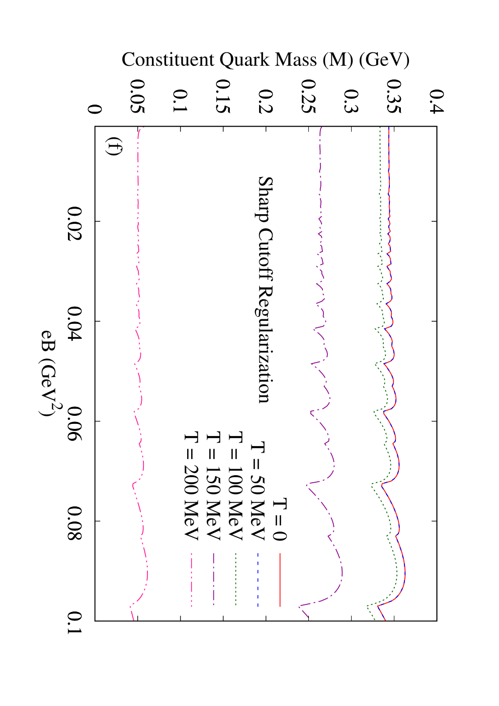
We now show the numerical results for the AMM of the quarks ($\kappa_{f}$) and the constituent quark mass ($M$) which are obtained by solving the coupled gap Eqs. (32)-(34) numerically. For all the numerical calculations, we have taken up to 1000 quark Landau levels. In Fig. 2, the variation of $\kappa_{\text{u}}$, $\kappa_{\text{d}}$ and $M$ as a function of temperature and external magnetic field are shown using the sharp cutoff regularization. We first notice from Figs. 2(a), (c) and (e), that both the AMM and constituent mass of the quarks are large in the chiral symmetry broken phase in the low temperature region. With the increase in temperature, they first remain almost unchanged up to a certain value of temperature and then fall rapidly around the pseudo-chiral phase transition temperature. Finally, at sufficiently high temperature region, the AMM of the quarks approach asymptotically to zero value whereas the constituent quark mass approaches the current quark mass value in the chiral symmetry restored phase. The temperature variation of the constituent quark mass in Fig. 2(e) is understandable physically from the fact that the mass gap $(M-m)$ is proportional to the chiral condensate $\langle\overline{\psi}\psi\rangle$, which is non-zero (zero) at the symmetry broken (restored) phase. Moreover, on comparing the finite magnetic field curves (blue, green and violet) with the zero magnetic field curve (red) in Fig. 2(e), we see that the external magnetic field strengthens the chiral condensate at all temperatures. This can also be noticed in Fig. 2(f) in which an overall increase of the constituent quark mass with the increase in magnetic field is seen.

On the other hand, the temperature dependence of the AMM of the quarks at zero magnetic field ( i.e. the red curves of Figs. 2(a), (c)) can be understood from Eqs. (16) and (30) where the AMM has a linear and dominant $M$ dependence apart from the complicated integral factor. Therefore, the temperature dependence of the AMM at zero magnetic field is almost similar to the temperature dependence of the constituent quark mass. Moreover, in the high temperature limit, the integral factor of Eq. (16) approaches to zero and we get $\kappa_{\text{u}}\simeq\kappa_{\text{d}}\simeq 0$. At non-zero external magnetic field, a linear $M$ dependence in the expression of AMM is not apparent from Eq. (27) unlike the zero magnetic field case and the RHS of Eq. (27) contains explicit AMM dependence as well as an implicit AMM dependence through the $M=M(\kappa)$. These complications forbid us to perform an analytical analysis of the finite magnetic field expressions. Nevertheless, numerically we see that, at sufficiently small value of external magnetic field, the complicated non-zero magnetic field expressions boil down to the exact zero-magnetic field results (compare the blue and red curves in Figs. 2(a), (c)); this is the consequence of the fact that at $B\simeq 0$, the Landau levels become infinitesimally close to each other and approach the continuum result of $B=0$.

Comparing Figs. 2(b) and (d), we see that AMM of the quarks are also slowly varying function of the external magnetic field alike the constituent quark mass depicted in Fig. 2(f). $\kappa_{\text{u}}$ decreases with the increase in external magnetic field whereas, $\kappa_{\text{d}}$ shows an opposite trend. This is due to the opposite signs of the charges of up and down quarks producing an opposite response to the external magnetic field.

In Figs. 2(b), (d) and (f), we notice that both the AMM as well as the constituent quark mass suffer oscillations as the magnetic field changes. These oscillations appear to be an artifact of the use of sharp three-momentum regulator as commented in Refs. Fukushima et al. 2010; Miransky and Shovkovy 2015. We also notice that, the amplitudes of these oscillations are maximum around the pseudo-chiral phase transition region. Interestingly, it turns out that, when we use the smooth cutoff regularization scheme, these unphysical oscillations vanish as depicted in Fig. 3. Comparing Fig. 2 and Fig. 3, we notice that, the oscillations appearing in Figs. 2(b), (d) and (f) get smeared out in Figs. 3(b), (d) and (f) keeping the overall qualitative and quantitative nature same. Moreover, the temperature dependence of AMM and constituent quark mass in Figs. 2(a), (c) and (e) suffers marginal change while switching to the smooth cutoff scheme as can be observed by comparing with Figs. 3(a), (c) and (e) respectively.

In summary, using a gauged NJL model, we have evaluated the effective photon-quark-antiquark ($\gamma q\overline{q}$) vertex function in the mean field approximation. The lowest order diagram that contributes to the magnetic form factor and the AMM of the quarks is calculated at finite temperature in presence of arbitrary external magnetic field. The incorporation of finite temperature is done through the ITF of finite temperature field theory where the continuous energies of the loop particles are replaced with discrete Matsubara modes. The complete (including all the Landau levels) Schwinger propagator with non-zero AMM of the dressed quarks are considered while calculating the loop graphs. Using two different momentum cutoff (sharp and smooth) regularization scheme, we regularize the UV divergences arising from the vertex function and the parameters of our model are chosen to reproduce the well known phenomenological quantities at zero temperature and zero magnetic field, such as pion-decay constant ($f_{\pi}$), vacuum quark condensate, vacuum pion mass ($m_{\pi}$) as well as the magnetic moments of proton and neutron using CQM. Finally, the temperature as well as magnetic field dependence of the AMM and constituent quark mass are studied.

Since the Schwinger propagator itself contains explicit AMM dependence, the magnetic form factor obtained from the vertex function in presence of magnetic field is also an explicit function of $\kappa$; along with, an implicit AMM dependence emerging from the constituent quark mass $M=M(\kappa)$. For this, the calculation of the AMM from the magnetic form factors requires solving a set of three coupled gap equations.

References

- Kharzeev et al. (2013) D. E. Kharzeev, K. Landsteiner, A. Schmitt, and H.-U. Yee, Lect. Notes Phys. 871, 1 (2013), arXiv:1211.6245 [hep-ph] .
- Vachaspati (1991) T. Vachaspati, Phys. Lett. B265, 258 (1991).
- Campanelli (2013) L. Campanelli, Phys. Rev. Lett. 111, 061301 (2013), arXiv:1304.6534 [astro-ph.CO] .
- Duncan and Thompson (1992) R. C. Duncan and C. Thompson, Astrophys. J. 392, L9 (1992).
- Thompson and Duncan (1993) C. Thompson and R. C. Duncan, Astrophys. J. 408, 194 (1993).
- Lai and Shapiro (1991) D. Lai and S. L. Shapiro, Astrophys. J. 383, 745 (1991).
- Kharzeev et al. (2008) D. E. Kharzeev, L. D. McLerran, and H. J. Warringa, Nucl. Phys. A803, 227 (2008), arXiv:0711.0950 [hep-ph] .
- Skokov et al. (2009) V. Skokov, A. Yu. Illarionov, and V. Toneev, Int. J. Mod. Phys. A24, 5925 (2009), arXiv:0907.1396 [nucl-th] .
- Tuchin (2013) K. Tuchin, Phys. Rev. C 88, 024911 (2013).
- Gursoy et al. (2014) U. Gursoy, D. Kharzeev, and K. Rajagopal, Phys. Rev. C89, 054905 (2014), arXiv:1401.3805 [hep-ph] .
- Tuchin (2016) K. Tuchin, Phys. Rev. C 93, 014905 (2016).
- Das et al. (2017) A. Das, S. S. Dave, P. S. Saumia, and A. M. Srivastava, Phys. Rev. C 96, 034902 (2017).
- Fukushima et al. (2008) K. Fukushima, D. E. Kharzeev, and H. J. Warringa, Phys. Rev. D78, 074033 (2008), arXiv:0808.3382 [hep-ph] .
- Kharzeev and Warringa (2009) D. E. Kharzeev and H. J. Warringa, Phys. Rev. D80, 034028 (2009), arXiv:0907.5007 [hep-ph] .
- Bali et al. (2012a) G. S. Bali, F. Bruckmann, G. Endrodi, Z. Fodor, S. D. Katz, S. Krieg, A. Schafer, and K. K. Szabo, JHEP 02, 044 (2012a), arXiv:1111.4956 [hep-lat] .
- Shovkovy (2013) I. A. Shovkovy, Lect. Notes Phys. 871, 13 (2013), arXiv:1207.5081 [hep-ph] .
- Gusynin et al. (1994) V. P. Gusynin, V. A. Miransky, and I. A. Shovkovy, Phys. Rev. Lett. 73, 3499 (1994), [Erratum: Phys. Rev. Lett.76,1005(1996)], arXiv:hep-ph/9405262 [hep-ph] .
- Gusynin et al. (1996) V. P. Gusynin, V. A. Miransky, and I. A. Shovkovy, Nucl. Phys. B462, 249 (1996), arXiv:hep-ph/9509320 [hep-ph] .
- Gusynin et al. (1999) V. P. Gusynin, V. A. Miransky, and I. A. Shovkovy, Nucl. Phys. B563, 361 (1999), arXiv:hep-ph/9908320 [hep-ph] .
- Preis et al. (2011) F. Preis, A. Rebhan, and A. Schmitt, JHEP 03, 033 (2011), arXiv:1012.4785 [hep-th] .
- Preis et al. (2013) F. Preis, A. Rebhan, and A. Schmitt, Lect. Notes Phys. 871, 51 (2013), arXiv:1208.0536 [hep-ph] .
- Elmfors et al. (1998) P. Elmfors, K. Enqvist, and K. Kainulainen, Phys. Lett. B440, 269 (1998), arXiv:hep-ph/9806403 [hep-ph] .
- Skalozub and Bordag (2000) V. Skalozub and M. Bordag, Int. J. Mod. Phys. A15, 349 (2000), arXiv:hep-ph/9904333 [hep-ph] .
- Sadooghi and Anaraki (2008) N. Sadooghi and K. S. Anaraki, Phys. Rev. D78, 125019 (2008), arXiv:0805.0078 [hep-ph] .
- Navarro et al. (2010) J. Navarro, A. Sanchez, M. E. Tejeda-Yeomans, A. Ayala, and G. Piccinelli, Phys. Rev. D82, 123007 (2010), arXiv:1007.4208 [hep-ph] .
- Fayazbakhsh and Sadooghi (2010) S. Fayazbakhsh and N. Sadooghi, Phys. Rev. D82, 045010 (2010), arXiv:1005.5022 [hep-ph] .
- Fayazbakhsh and Sadooghi (2011) S. Fayazbakhsh and N. Sadooghi, Phys. Rev. D83, 025026 (2011), arXiv:1009.6125 [hep-ph] .
- Skokov (2012) V. Skokov, Phys. Rev. D85, 034026 (2012), arXiv:1112.5137 [hep-ph] .
- Fukushima and Pawlowski (2012) K. Fukushima and J. M. Pawlowski, Phys. Rev. D86, 076013 (2012), arXiv:1203.4330 [hep-ph] .
- Chernodub (2011) M. N. Chernodub, Phys. Rev. Lett. 106, 142003 (2011), arXiv:1101.0117 [hep-ph] .
- Chernodub et al. (2012) M. N. Chernodub, J. Van Doorsselaere, and H. Verschelde, Phys. Rev. D85, 045002 (2012), arXiv:1111.4401 [hep-ph] .
- Bazavov et al. (2017) A. Bazavov, H.-T. Ding, P. Hegde, O. Kaczmarek, F. Karsch, E. Laermann, Y. Maezawa, S. Mukherjee, H. Ohno, P. Petreczky, H. Sandmeyer, P. Steinbrecher, C. Schmidt, S. Sharma, W. Soeldner, and M. Wagner, Phys. Rev. D 95, 054504 (2017).
- Guenther et al. (2017) J. N. Guenther, R. Bellwied, S. Borsanyi, Z. Fodor, S. D. Katz, A. Pasztor, C. Ratti, and K. K. Szabó, Proceedings, 26th International Conference on Ultra-relativistic Nucleus-Nucleus Collisions (Quark Matter 2017): Chicago, Illinois, USA, February 5-11, 2017, Nucl. Phys. A967, 720 (2017), arXiv:1607.02493 [hep-lat] .
- Bazavov et al. (2012) A. Bazavov, T. Bhattacharya, M. Cheng, C. DeTar, H.-T. Ding, S. Gottlieb, R. Gupta, P. Hegde, U. M. Heller, F. Karsch, E. Laermann, L. Levkova, S. Mukherjee, P. Petreczky, C. Schmidt, R. A. Soltz, W. Soeldner, R. Sugar, D. Toussaint, W. Unger, and P. Vranas (HotQCD Collaboration), Phys. Rev. D 85, 054503 (2012).
- Bazavov et al. (2014) A. Bazavov, T. Bhattacharya, C. DeTar, H.-T. Ding, S. Gottlieb, R. Gupta, P. Hegde, U. M. Heller, F. Karsch, E. Laermann, L. Levkova, S. Mukherjee, P. Petreczky, C. Schmidt, C. Schroeder, R. A. Soltz, W. Soeldner, R. Sugar, M. Wagner, and P. Vranas (HotQCD Collaboration), Phys. Rev. D 90, 094503 (2014).
- Brandt et al. (2016) B. B. Brandt, G. Bali, G. Endrödi, and B. Glässle, Proceedings, 33rd International Symposium on Lattice Field Theory, PoS LATTICE2015, 265 (2016), arXiv:1510.03899 [hep-lat] .
- Bali et al. (2012b) G. S. Bali, F. Bruckmann, G. Endrodi, Z. Fodor, S. D. Katz, and A. Schafer, Phys. Rev. D86, 071502 (2012b), arXiv:1206.4205 [hep-lat] .
- Sharma (2019) S. Sharma, Proceedings, 36th International Symposium on Lattice Field Theory (Lattice 2018): East Lansing, MI, United States, July 22-28, 2018, PoS LATTICE2018, 009 (2019), arXiv:1901.07190 [hep-lat] .
- Andersen et al. (2016) J. O. Andersen, W. R. Naylor, and A. Tranberg, Rev. Mod. Phys. 88, 025001 (2016), arXiv:1411.7176 [hep-ph] .
- Nambu and Jona-Lasinio (1961a) Y. Nambu and G. Jona-Lasinio, Phys. Rev. 124, 246 (1961a), [,141(1961)].
- Nambu and Jona-Lasinio (1961b) Y. Nambu and G. Jona-Lasinio, Phys. Rev. 122, 345 (1961b), [,127(1961)].
- Klevansky (1992) S. P. Klevansky, Rev. Mod. Phys. 64, 649 (1992).
- Hatsuda and Kunihiro (1994) T. Hatsuda and T. Kunihiro, Phys. Rept. 247, 221 (1994), arXiv:hep-ph/9401310 [hep-ph] .
- Vogl and Weise (1991) U. Vogl and W. Weise, Prog. Part. Nucl. Phys. 27, 195 (1991).
- Buballa (2005) M. Buballa, Phys. Rept. 407, 205 (2005), arXiv:hep-ph/0402234 [hep-ph] .
- Klevansky and Lemmer (1989) S. P. Klevansky and R. H. Lemmer, Phys. Rev. D39, 3478 (1989).
- Mao (2016) S. Mao, Phys. Lett. B758, 195 (2016), arXiv:1602.06503 [hep-ph] .
- Fayazbakhsh et al. (2012) S. Fayazbakhsh, S. Sadeghian, and N. Sadooghi, Phys. Rev. D86, 085042 (2012), arXiv:1206.6051 [hep-ph] .
- Ruggieri et al. (2013) M. Ruggieri, M. Tachibana, and V. Greco, JHEP 07, 165 (2013), arXiv:1305.0137 [hep-ph] .
- Ghosh et al. (2020a) S. Ghosh, A. Mukherjee, N. Chaudhuri, P. Roy, and S. Sarkar, Phys. Rev. D 101, 056023 (2020a), arXiv:2003.02024 [hep-ph] .
- Avancini et al. (2019a) S. S. Avancini, R. L. S. Farias, and W. R. Tavares, Phys. Rev. D99, 056009 (2019a), arXiv:1812.00945 [hep-ph] .
- Avancini et al. (2019b) S. S. Avancini, R. L. S. Farias, N. N. Scoccola, and W. R. Tavares, Phys. Rev. D 99, 116002 (2019b).
- Avancini et al. (2012) S. S. Avancini, D. P. Menezes, M. B. Pinto, and C. m. c. Providência, Phys. Rev. D 85, 091901 (2012).
- Zhang et al. (2016) R. Zhang, W.-j. Fu, and Y.-x. Liu, Eur. Phys. J. C76, 307 (2016), arXiv:1604.08888 [hep-ph] .
- Peskin and Schroeder (1995) M. E. Peskin and D. V. Schroeder, An Introduction to quantum field theory (Addison-Wesley, Reading, USA, 1995).
- Schwartz (2013) M. D. Schwartz, Quantum Field Theory and the Standard Model (Cambridge University Press, 2013).
- Schwinger (1948) J. Schwinger, Phys. Rev. 73, 416 (1948).
- Mohr et al. (2008) P. J. Mohr, B. N. Taylor, and D. B. Newell, Rev. Mod. Phys. 80, 633 (2008).
- Mao and Rischke (2019) S. Mao and D. H. Rischke, Phys. Lett. B 792, 149 (2019), arXiv:1812.06684 [hep-th] .
- Ferrer and de la Incera (2009) E. J. Ferrer and V. de la Incera, Phys. Rev. Lett. 102, 050402 (2009).
- Ferrer and [de la Incera] (2010) E. J. Ferrer and V. [de la Incera], Nuclear Physics B 824, 217 (2010).
- Ferrer et al. (2015) E. J. Ferrer, V. de la Incera, D. M. Paret, A. P. Martínez, and A. Sanchez, Phys. Rev. D 91, 085041 (2015).
- Singh (1985) J. P. Singh, Phys. Rev. D 31, 1097 (1985).
- Halzen and Martin (1984) F. Halzen and A. D. Martin, QUARKS AND LEPTONS: AN INTRODUCTORY COURSE IN MODERN PARTICLE PHYSICS (1984).
- Bicudo et al. (1999) P. J. Bicudo, J. F. Ribeiro, and R. Fernandes, Phys. Rev. C 59, 1107 (1999), arXiv:hep-ph/9806243 .
- Fayazbakhsh and Sadooghi (2014) S. Fayazbakhsh and N. Sadooghi, Phys. Rev. D90, 105030 (2014), arXiv:1408.5457 [hep-ph] .
- Chaudhuri et al. (2019) N. Chaudhuri, S. Ghosh, S. Sarkar, and P. Roy, Phys. Rev. D99, 116025 (2019), arXiv:1907.03990 [nucl-th] .
- Chaudhuri et al. (2020) N. Chaudhuri, S. Ghosh, S. Sarkar, and P. Roy, Eur. Phys. J. A 56, 213 (2020), arXiv:2003.05692 [nucl-th] .
- Ghosh et al. (2020b) S. Ghosh, N. Chaudhuri, S. Sarkar, and P. Roy, Phys. Rev. D 101, 096002 (2020b), arXiv:2004.09203 [nucl-th] .
- Mei and Mao (2020) J. Mei and S. Mao, Phys. Rev. D 102, 114035 (2020), arXiv:2008.12123 [hep-ph] .
- Fukushima et al. (2010) K. Fukushima, M. Ruggieri, and R. Gatto, Phys. Rev. D 81, 114031 (2010), arXiv:1003.0047 [hep-ph] .
- Miransky and Shovkovy (2015) V. A. Miransky and I. A. Shovkovy, Phys. Rept. 576, 1 (2015), arXiv:1503.00732 [hep-ph] .