A Bayesian Modified Ising Model for Identifying Spatially Variable Genes from Spatial Transcriptomics Data
Abstract
Abstract
A recent technology breakthrough in spatial molecular profiling has enabled the comprehensive molecular characterizations of single cells while preserving spatial information. It provides new opportunities to delineate how cells from different origins form tissues with distinctive structures and functions. One immediate question in spatial molecular profiling data analysis is to identify genes whose expressions exhibit spatially correlated patterns, called spatially variable genes. Most current methods to identify spatially variable genes are built upon the geostatistical model with Gaussian process to capture the spatial patterns, which rely on ad hoc kernels that could limit the models’ ability to identify complex spatial patterns. In order to overcome this challenge and capture more types of spatial patterns, we introduce a Bayesian approach to identify spatially variable genes via a modified Ising model. The key idea is to use the energy interaction parameter of the Ising model to characterize spatial expression patterns. We use auxiliary variable Markov chain Monte Carlo algorithms to sample from the posterior distribution with an intractable normalizing constant in the model. Simulation studies using both simulated and synthetic data showed that the energy-based modeling approach led to higher accuracy in detecting spatially variable genes than those kernel-based methods. When applied to two real spatial transcriptomics datasets, the proposed method discovered novel spatial patterns that shed light on the biological mechanisms. In summary, the proposed method presents a new perspective for analyzing spatial transcriptomics data.
Keywords: Spatial molecular profiling; Multitype point pattern; Spatial correlation, Dichotomization; Double Metropolis-Hastings
I Introduction
Cellular and molecular spatial organizations play essential roles in biological functions. In recent years, spatial molecular profiling (SMP) techniques have made significant breakthroughs, which enable transcriptome measurement in high spatial resolution (Zhang and others 2020). Gene expression profiling approaches are no longer limited tissue-dissociation, which led to the loss of spatial context of the measured gene expression (Femino and others 1998). Sequencing-based spatial molecular profiling platforms, such as spatial transcriptomics (ST) (Ståhl and others 2016) and the improved Visium platform, use spatial barcodes to capture RNA molecules and then synthesize and sequence their complementary DNA molecules. Through this technology, the expression levels of thousands of genes can be measured across hundreds of spatial locations, namely spots. Those spots are usually arrayed on a two-dimensional grid. Particularly, ST and Visium spots are arranged on the square and triangular lattices, respectively.
SMP techniques enable researchers to study the gene expressions together with their spatial and morphological contexts, which provide new opportunities to advance our understanding of both cellular and molecular spatial organizations (Crosetto and others 2015), and their relationships with diseases (Shah and others 2018). Many new questions can be explored with the emerging SMP techniques. One of the most immediate ones is to identify genes whose expressions exhibit spatially correlated patterns, referred to spatially variable (SV) genes. The study of spatial patterns in gene expression could reveal significant insights into many aspects, such as embryo development (Satija and others 2015), tumor progression (de Bruin and others 2014), and the clinical impact of intra-tumor heterogeneity (Bedard and others 2013).
Several methods have been developed in recent years to address the above fundamental question in ST studies. Trendsceek (Edsgärd and others 2018) is based on marked point processes, and it is computationally intensive (Dries and others 2021) and has noticeably unsatisfying performance (Sun and others 2020). BinSpect (Dries and others 2021) is an easy and fast computational method based on statistical enrichment of spatial network neighbors after binarizing gene expression levels. Most model-based analyses, such as SPARK (Sun and others 2020), SpatialDE (Svensson and others 2018), and BOOST-GP (Li and others 2021), are built upon the geostatistical model with Gaussian process (GP), where a kernel must be selected with caution. Among these methods, SpatialDE transforms the measured counts at different locations into normalized data before analysis, SPARK uses a Poisson distribution to model the count data directly, and BOOST-GP accounts for the zero-inflation and mean-variance relationship existed in raw counts under a Bayesian framework. However, the GP-based models rely on ad hoc kernels that limit the models’ ability to identify complex spatial patterns. Furthermore, none of the existing approaches take advantage of the additional spatial structure of the ST data; that is, the gene expression levels are measured on a lattice grid.
To enable the model to identify complex spatial patterns, we developed a novel approach named Bayesian mOdeling Of Spatial Transcriptomics data via a Modified Ising model (BOOST-MI) to identify SV genes in ST studies. It makes computation efficient by taking advantage of the fact that the ST experiments measure gene expression on a lattice. Ahead of fitting BOOST-MI, we need to normalize sequence count data to relative gene expression levels and dichotomize relative expression levels to a binary spatial pattern. Then, BOOST-MI characterizes the binary spatial pattern via inferring the Ising model interaction parameter under a Bayesian framework. The double Metropolis-Hastings (DMH) algorithm (Liang 2010) is used to sample from the posterior distribution with an intractable normalizing constant in the Ising model. Compared with other existing approaches, BOOST-MI tests the interaction energy parameter in a modified Ising model, which is able to characterize a broader type of spatial patterns than kernel-based modeling approaches. In addition, the proposed method enriches the inference via incorporating priors if necessary and naturally quantifying uncertainties under a Bayesian framework. We demonstrated the advantages of BOOST-MI in a comprehensive simulation study using both simulated data with various spatial patterns and zero-inflation settings and synthetic data from real ST experiments. The proposed model showed an outstanding performance compared to the alternatives. Finally, when applied to two real ST datasets, the proposed method discovered novel spatial patterns that shed light on the biological mechanisms.
The remainder of the paper is organized as follows. Section 2 introduces the two main components of the data preparation for BOOST-MI: sequence count data normalization and relative expression level dichotomization. In Sections 3 and 4, we introduce the proposed modeling framework and describe the Markov chain Monte Carlo (MCMC) algorithm and the resulting posterior inference. In Section 5, we compare BOOST-MI with existing approaches on simulated and two real ST datasets. Section 6 concludes the paper and discusses future research directions.
II Data Preparation
In this section, we introduce the two data preprocessing steps (see the dashed-line block in Figure 1) before fitting BOOST-MI to identify SV genes. We first summarize the ST data notations. Let an matrix denote the gene expression count table (i.e. the molecular profile). Each entry is the read count for gene collected at spot . We use an matrix to represent the geospatial profile, where each row indicates the spot location on the two-dimensional space. All non-boundary spots have the same neighborhood structure. Suppose the gene expression levels are measured on a -by- square lattice grid, the coordinate of each spot can be written as . If it is not a boundary spot, then its four neighboring spots are at locations and .
Normalization is critical to sequence count data analysis. To counteract various artifacts and bias due to biological and technical reasons, we convert each read count to its relative gene expression level, denoted by , where is the size factor of sample , capturing all nuisance effects. The most straightforward way is to set , i.e. the total number of counts across all genes in each sample (known as sequencing depth or library size), combined with some constraint, such as . Note that SPARK suggests this normalization, namely total sum scaling (TSS). We could also consider other estimations on ’s, which have been introduced for mitigating the influence of extremely low and high counts when analyzing bulk RNA-seq data, such as upper-quartiles (Q75) (Bullard and others 2010), relative log expression (RLE) (Anders and Huber 2010), and weighted trimmed mean by M-values (TMM) (Robinson and Oshlack 2010). In addition to the above normalization method based on size factor estimation, we could use the method based on variance-stabilizing transformation (VST) (detailed in Section S1 in the supplement). A following sensitivity analysis (see Figure S1 in the supplement) indicates that 1) the methods based on size factor estimation noticeably outperformed the VST-based methods; 2) the performance based on TSS was not significantly different from Q75, RLE, and TMM. Thus, we suggest using TSS as the default setting for the sake of simplicity.
We then denoise the relative expression levels by partitioning all spots into two groups. This step outputs the suitable data type required in the subsequent analysis and makes our approach more robust in the face of over-dispersion and zero-inflation, which are the two important characteristics of ST data. For each gene, we introduce a binary vector to represent the dichotomization result based on its relative expression levels , with indicating gene is highly expressed at spot and otherwise. Since there is no consensus on the dichotomization of spots based on either absolute or relative expression level, we propose to estimate via fitting a two-component Gaussian mixture model (GMM), , subjecting to . Here and are the group means and variances that need to be estimated. In addition to the model-based clustering, we also consider -means, which is implicitly based on pairwise distances between relative expression levels. Section S2 in the supplement provides details about the GMM and -means implementations (). A following sensitivity analysis (see Figure S2 in the supplement) indicates that BOOST-MI performed equally well between the two choices.
III Models
In this section, we first review the Ising model and then introduce a modified Ising model with external fields to identify SV genes. The schematic diagram is shown in Figure 1.
III.1 A brief review of the Ising model
The Ising model, first introduced by Lenz 1920 and used in statistical mechanics, is a model of interacting binary states on a crystalline lattice (Cipra 1987). Let denote a graph with a finite set of vertices and a set of edges . In statistics, the Ising model is considered as an undirected graph such that each vertex is geometrically regular assigned on a lattice and each edge is of the same length (Tucker 1994). There are three typical types of two-dimensional lattices: square, triangular, and honeycomb (see Figure 2). The former two are a special case of Bravais lattices, which can be defined as an infinite array of discrete points generated by a set of discrete translation operations (Ashcroft and others 1976). ST and Visium (an improved ST platform) spots are arranged on square and triangular lattices, where each non-boundary spot has four and six neighbors, respectively. Every vertex will be assigned a binary state (also known as a spin). If there are three or more states, the model is known as the Potts model. Because the spots are assigned with different spins and react with their neighbors’ spins, there exists a measurement of overall energy, named Hamiltonian,
| (1) |
where denotes the collection of all neighboring spot pairs, denotes the interaction energy between highly and lowly expressed spots for gene , and denotes the indicator function. According to the Hammersley–Clifford theorem (Clifford 1990), we can write the probability of observing a particular configuration of as , where denotes the set of all configurations of spins. An exact evaluation of the normalizing constant (i.e. the denominator of the above equation) requires us to sum over the entire space, consisting of configurations. Thus, is intractable even for a small lattice size.
III.2 A proposal of using a modified Ising model to identify SV genes
Although Ising models have a wide range of applications in many areas, they are often examined assuming that the underlying abundance of different spins is equivalent. In the context of statistical mechanics, we can view the model as a system of interacting particles in the absence of an external field. However, we found that low-expression spots are usually much higher than high-expression spots due to excessive zeros presented in the ST data. For instance, the averaged proportions of low-expression spots in the two processed real ST datasets analyzed in the paper were and , respectively (see Figure S3 in the supplement). Ignoring this feature could decrease the identification accuracy due to the inclusion of more false positives (see Figure 4).
To remedy the oversimplified Ising model, we add an external force in the Hamiltonian,
| (2) |
where and represent the first and second-order intensities. The first term is proportional to the number of neighboring spot pairs with different spins, while the remaining part (in the square bracket) can be viewed as the weighted average of the numbers of spots with different spins. As the energy function in Equation (2) is still locally defined, we can write the joint probability on , up to its normalizing constant, as
| (3) |
which serves as the full data likelihood of the proposed BOOST-MI model. To interpret and , we give the conditional probability of observing a high-expression level of gene at spot ,
| (4) |
where denotes the set of all neighbors to spot . Equation (4) is essentially a logistic regression, and hence the parameters and can be interpreted in terms of conditional odds ratios in general. According to Equation (4), if , then , implying that each dichotomized expression level is independently and identically sampled from a Bernoulli distribution. Thus, no spatial pattern should exhibit, and gene is a non-SV gene. The underlying abundance of low and high-expression levels in are characterized by and , respectively. Fixing , Equation (4) reveals that the smaller the (i.e. ), the more likely the dichotomized expression level at any spot is concordant with the majority of its neighboring spots’ levels, resulting in a repulsion pattern (i.e. the clustering of spots with the same dichotomized expression level). In contrast, when takes a large positive value, we expect an attraction pattern; that is, the exhibition of clustering among spots with different dichotomized expression levels. Thus, the spatial correlation between the low and high-expression levels of gene can be quantified by . Figure 1 shows the three typical patterns in terms of conditional on .
In conclusion, BOOST-MI uses to characterize the binary spatial pattern defined by the dichotomized gene expression levels on the lattice grid . It is noteworthy that the kernel-based methods, such as SPARK, SpatialDE, and BOOST-GP, are only able to identify SV genes with a small subset of repulsion patterns defined by the selected kernel, while BOOST-MI accounts for all attraction and repulsion patterns.
To complete the model specification, we impose . As for the first-order intensity , we notice that an identifiability problem arises from Equation(4). For example, adding a nonzero constant into does not change the conditional probability . Thus, we force and set a normal prior on .
IV Model Fitting
In this section, we describe the MCMC algorithm for model fitting and the posterior inference. Our inferential strategy allows for simultaneously estimating the first-order intensity , which reveals the underlying abundance of the low and high-expression levels of gene , and the second-order intensity (also known as the interaction parameter), which captures the spatial correlation between the low and high-expression levels. We give the details of our MCMC algorithm and the resulting posterior inference as below. Note that each gene is tested independently by BOOST-MI.
IV.1 MCMC algorithm
The full data likelihood function is given in Equation (3), which involves an intractable normalizing constant . Taking the two real ST datasets analyzed in the paper as examples, it needs to sum over and elements, respectively. This makes the Metropolis–Hastings (MH) algorithm infeasible in practice. To overcome this challenge, we employ the double MH (DMH) algorithm (Liang 2010) to estimate both and for each gene. The DMH is an asymptotic algorithm, which has been shown to produce accurate results by various spatial models (Li and others 2019a; Li and others 2019b). Unlike other auxiliary variable MCMC algorithms (Møller and others 2006; Murray and others 2012) that also aim to have the normalizing constant ratio canceled, it is more efficient because it does not require drawing the auxiliary variables from a perfect sampler, which is usually computationally expensive.
To update within each iteration, we first simulate a new sample from using the MH algorithm starting with . Then, we generate an auxiliary variable through MH updates starting with the current state based on the new value and accept it with probability , where . If the auxiliary variable is accepted, we update to ; otherwise, we keep the value of . No improvement in the performance was noticed beyond in both simulation and application studies of this paper.
Just as in updating , we use the DMH algorithm to update . Specifically, we first simulate a new sample from using the MH algorithm starting with . Then, we generate an auxiliary variable through MH updates starting with the current state based on the new value and accept it with probability , where . If the auxiliary variable is accepted, we update to ; otherwise, the value of remains the same.
IV.2 Posterior inference
Our primary interest lies in the identification of SV genes via making inferences on the interaction parameter . We obtain the posterior inference by post-processing of the MCMC samples after burn-in. To validate if gene exhibits a repulsion pattern, we set the null and alternative hypotheses as and ; while testing an attraction pattern, we set and . We could select the model via calculating the Bayes factor (BF) in favor of over , which is defined as the ratio of posterior odds to prior odds,
| (5) |
where the prior odds cancel out as we choose a normal prior on centered at zero, and the posterior odds can be approximated using the MCMC samples . Here denotes the total number of MCMC iterations after burn-in. The larger the , the more likely gene is an SV gene, integrating over the uncertainty in all model parameters. We suggest choosing the BF threshold based on the scale for interpretation (Kass and Raftery 1995).
V Results
V.1 Simulation
We performed a series of simulation studies to evaluate the performance of BOOST-MI and compared it with that of four existing methods: SpatialDE, SPARK, BOOST-GP, and BinSpect. Because of the poor performance of Trendsceek reported in most literature (Sun and others 2020; Dries and others 2021), we did not include it here. In addition, we fitted the classic Ising model (with the Hamiltonian defined in Equation (1)) under the same Bayesian framework.
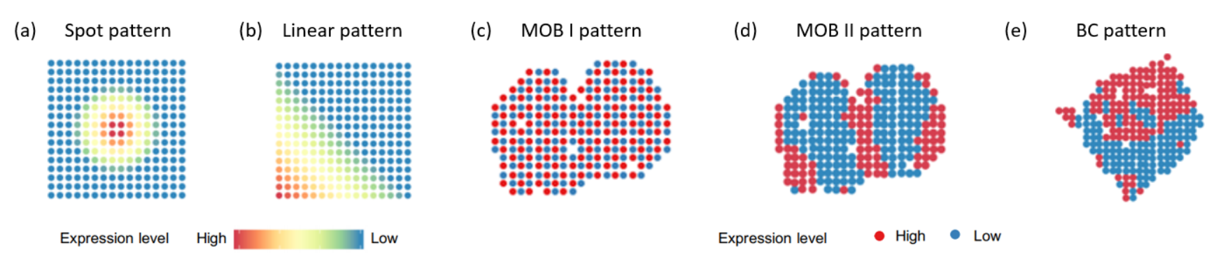
We generated simulated data from three artificial spatial patterns (see Figure 3(a)-(c)) and two real spatial patterns (see Figure 3(d) and (e)). The two real patterns were constructed from the mouse olfactory bulb (MOB) and human breast cancer (BC) datasets analyzed in this paper. The first two artificial patterns named spot and linear were on a square lattice ( spots), while the remaining one named MOB I was on spots. The MOB II and BC patterns were on and spots, respectively. We set , among which were SV genes. We followed the data generative schemes (Edsgärd and others 2018; Sun and others 2020; Li and others 2021) to simulate the gene expression count table , which was substantially different from the model assumptions of BOOST-MI. For each gene , the log relative expression level at spot was generated via
where denotes the baseline relative expression level and denotes the non-spatial errors following . We set and . For a non-SV gene, the relative expression levels were from a log-normal (LN) distribution with mean and variance being and . Consequently, no spatial correlation should be observed. For an SV gene with the spot pattern, the values of ’s of the four center spots at , , , and were set to , while all others were linearly decreased to zero within a radius of five spots. For an SV gene with the linear pattern, the value of of the most bottom-left spot at was set to , while all others were linearly decreased to zero along the diagonal line. For an SV gene with the remaining patterns, each spot was dichotomized into low and high-expression levels with and , respectively. To mimic the excess zeros and over-dispersion in the real ST datasets, we sampled each gene expression count from a zero-inflated negative binomial (ZINB) model, , where the size factor and the dispersion parameter was from an exponential distribution with mean . For the choice of the false zero proportion , we randomly selected , , or counts and forced their values to zero. Combined with the five patterns and three zero-inflation settings, there were different scenarios. For each scenario, we repeated the above steps to generate replicates.
We chose to normalize the raw counts using TSS and dichotomize the relative expression levels for each gene using GMM as the default setting. As for BOOST-MI, the prior specification are and . We set and . The former indicated that the underlying proportion of the low-expression spots was expected between and with a probability of , while the latter ensured about of ’s value ranged from to a priori. A follow-up sensitivity analysis indicated that BOOST-MI was incredibly insensitive to the choice of these two hyperparameters (see Section S3 and Figure S4 in the supplement). As for the MCMC algorithm, we ran four independent MCMC chains for each gene with iterations, discarding the first half as burn-in. We started each chain from a model by randomly drawing all parameters from their prior distributions. Results we report below were obtained by pooling together the MCMC outputs from the four chains.
Both BOOST-MI and BOOST-GP identify SV genes based on BFs, while BinSpect, SPARK and SpatialDE output -values to guide the selection. First, we used the area under the curve (AUC) of the receiver operating characteristic (ROC) to evaluate the performance of all methods. The ROC curve was created by plotting the true positive rate against the false positive rate across various thresholds used to select SV genes based on BFs or -values. Second, we classified each gene as an SV or non-SV gene by pinpointing a specified threshold. Specifically, we set the BF cutoff to , corresponding to a decisive strength of evidence. To control the type-I error rate, we adjusted -values from SPARK, SpatialDE, and BinSpect using the Benjamini-Hochberg method (Benjamini and Hochberg 1995) and chose a significance level of as the cutoff. We chose the Matthews correction coefficient (MCC) (Matthews 1975) as the secondary performance metric, because SV genes is usually only a small subset of all genes, making other binary classification metrics not suitable. AUC yields a value between and , and MCC value ranges from to . For both of them, the larger the value, the more accurate the identification.
According to Figure 4, which displays the boxplots of AUCs by different methods over ten replicated datasets under each scenario, we concluded as follows. First, BOOST-MI achieved the highest performance in terms of median AUC under out of scenarios, while BOOST-GP only had a marginal advantage over BOOST-MI under the scenario with a medium or high proportion of false zeros and the artificial spot or linear pattern. Second, under the low zero-inflation setting, SPARK had a similar performance with BOOST-MI when the SV genes were generated from linear and BC patterns. However, it suffered from reduced power under the medium and high zero-inflation settings. This clearly suggested that realistic modeling in BOOST-MI contributed to its advantage over all other methods. Third, BinSpect was very sensitive to the choice of clustering methods. For example, the one based on top percentage rank performed significantly better than the one based on -means under almost all scenarios, excluding the four scenarios with a high proportion of false zeros and the first four spatial patterns. In contrast, BOOST-MI is considerably robust to different normalization and dichotomization methods (see Figure S1 and S2 in the supplement). Forth, our BOOST-MI with the modified Hamiltonian consistently outperformed the Ising model with the classic Hamiltonian. Last but not least, SPARK, SpatialDE and BOOST-GP absolutely had no power to detect SV genes with the MOB I pattern, which was defined by a large positive interaction parameter in the Ising model. They might miss some important discoveries in real data analysis. Meanwhile, BinSpect had no satisfactory performance to detect such a pattern either, indicating our model-based analysis BOOST-MI could sharpen inferences. Besides, we reported the summaries of all methods’ performance in terms of MCCs in Figure S5 and Table S3 in the supplement, respectively. Those results led to similar conclusions.
Regarding the efficiency, the average execution time per gene was , , and seconds for BinSpect, SPARK, and SpatialDE. BOOST-MI spent seconds per gene on average due to the computationally intensive DMH algorithms. In contrast, BOOST-GP had around two times higher computational cost than BOOST-MI, which spent seconds per gene on average. All experiments were implemented on a high performance computing server with two Intel Xeon CPUs ( MB cache and GHz) and GB memory.
V.2 Application to mouse olfactory bulb ST dataset
The first dataset that we applied BOOST-MI to analyze is a publicly available ST dataset in a mouse olfactory bulb (MOB) study. It is accessible on the Spatial Research Lab (http://www.spatialresearch.org). There are replicates in this study. Following the previous studies (Svensson and others 2018; Sun and others 2020; Li and others 2021), we used the MOB replicate 11, which contains genes measured on spots. We applied the quality control steps described below before applying BOOST-MI. First, we excluded spots with fewer than ten total counts across all genes. Then, those genes with more than zero read counts across all spots were dropped. After these two steps, the MOB data had spots and genes. For other methods, we applied the pre-processing procedures suggested in their papers. We used the same prior specification, algorithm setting, and significance criteria used in the simulation study. We ran four independent MCMC chains and used the potential scale reduction factor (PSRF) (Gelman and others 1992) to diagnose MCMC convergence. PSRF is a statistic comparing the estimated between-chains and within-chain variances for a model parameter. Its value should be close to one if multiple chains have converged to the target posterior distribution. The PSRFs for all ’s and ’s were below , clearly suggesting that the MCMC algorithms converged. Then, for each dataset, we pooled together the outputs from the four chains and selected SV genes based on BFs. We only compared BOOST-MI with SPARK and BinSpect-rank due to the poor performance of SpatialDE and heavy computational burden of BOOST-GP.
BOOST-MI identified SV genes, which was approximately the same number of SV genes detected by SPARK ( SV genes) and around half of the number of SV genes detected by BinSpect ( SV genes). Figure 5(a) is a Venn diagram showing the overlap of detected SV genes by all methods. More than half of the SV genes identified by BOOST-MI ( out of ) were also reported by the other two, while there were unique SV genes to BOOST-MI. Most of the SV genes detected by SPARK ( out of ) were also included in the result of BOOST-MI or BinSpect, which indicates that SPARK is a relatively conservative method for SV gene identification. BinSpect was shown to be the most aggressive method that reported the most SV genes, more than half of which ( out of ) were not founded by either alternative.
To further explore the spatial patterns we had found, we performed the agglomerative hierarchical clustering on the SV genes identified by each of the three methods. For better visualization, we followed the data preprocessing (Svensson and others 2018; Sun and others 2020) to normalize the raw read counts to relative expression levels using log-VST. Next, based on the distance matrix computed from relative expression levels of all pairs of SV genes, a hierarchical clustering dendrogram was constructed. We then determined the number of clusters by cutting the hierarchical clustering dendrogram at a height corresponding to a clear separation. Last, we summarized the expression patterns via the averaged relative expression levels within each cluster. As a result, the SV genes detected by BOOST-MI and BinSpect were clustered into five groups, while there were four groups for SPARK, shown in Figure 5(b). Consistent with results in a previous study (Sun and others 2020), three major spatial patterns were shown in the first three columns in Figure 5(b). Note that the fourth pattern of SPARK (with genes) and BinSpect (with genes) could be merged into their first pattern, respectively. Also, the third and fourth patterns of BOOST-MI had a high similarity. It is noteworthy that a unique pattern (the last pattern of BOOST-MI) could only be detected by BOOST-MI with SV genes, indicating our method had a higher power. To further compare BOOST-MI with SPARK, we repeated the above procedure on those SV genes detected by BOOST-MI or SPARK only. The results are shown in Figure 5(c) and (d), respectively. The genes identified only by BOOST-MI could be categorized into two groups, including the unique pattern with genes. SV genes only detected by SPARK showed a strong periodic pattern, suggesting that SPARK might be more sensitive to the smooth periodic spatial pattern.
Next, using a Python wrapper GSEAPY (Subramanian and others 2007; Kuleshov and others 2016), we performed gene ontology (GO) enrichment analysis of the SV genes identified by BOOST-MI to explore their relevant biological functions. A total of mouse GO terms in three components (biological processes, cellular components, and molecular functions) had at least one gene overlap. Controlling the false discovery rate (FDR) at , we found GO terms, the top of which (with the smallest -values) are shown in Figure 5(f). As with SPARK, many enriched gene sets were related to synaptic signaling and the nervous system, both of which are significantly associated with the synaptic organization and olfactory bulb development (Treloar and others 2010). Examples include chemical synaptic transmission (GO:0007268; adjusted -value ) and nervous system development (GO:0007399; adjusted -value ).
Last but not least, BOOST-MI identified genes that had an attraction pattern with a positive interaction parameter in the Ising model. Table S4 in the supplement lists all of them. To analyze the potential biological functions of these SV genes, we performed functional enrichment analysis. There were mouse GO terms and Kyoto Encyclopedia of Genes and Genomes (KEGG) terms with at least one gene overlapping with those SV genes. We also found some statistically significant GO and KEGG terms, which had adjusted -values less than a significance level of . For example, holo TFIIH complex (GO:0005675) and nucleotide excision repair KEGG term were significantly enriched (adjusted -value and , respectively). In all, these discoveries highlighted the advantage of BOOST-MI.
V.3 Application to human breast cancer ST dataset
The second dataset is an available ST dataset in a human breast cancer (BC) study, which is also accessible on the Spatial Research Lab (http://www.spatialresearch.org). There are four layers available and we used the BC layer 2, which contains genes measured on spots. We applied the same quality control steps described in Section V.2. The BC data had spots and genes. We applied the same pre-processing procedures for other methods and the same prior specification, algorithm setting, and significance criteria as mentioned. To check convergence, we run four chains and the PSRFs for all ’s and ’s were below . We also compared our result with BinSpect and SPARK.
There were SV genes identified by BOOST-MI, which was slightly larger than the number of SV genes detected by SPARK ( SV genes) and around one-tenth of the number of SV genes detected by BinSpect ( SV genes). A Venn diagram, as shown in Figure 6(a), indicates that over of the SV genes detected by BOOST-MI ( out of ) were in common with the result obtained by both SPARK and BinSpect. There were only SV genes identified only by BOOST-MI. Once again, it demonstrated that SPARK is a conservative method and Binspect is an aggressive one, since nearly of the SV genes detected by SPARK ( out of ) were also included in the results of BOOST-MI or BinSpect, while nearly of the SV genes reported by BinSpect ( out of ) were found by neither BOOST-MI nor SPARK.
We reported more detailed analysis results, following the same procedure when studying the MOB dataset. Each row in Figure 6(b) shows the distinct expression patterns detected by BOOST-MI, SPARK, and BinSpect, respectively. There were five, four, and five groups obtained by performing the agglomerative hierarchical clustering. It is noteworthy that BOOST-MI detected all four patterns discovered by SPARK. However, BOOST-MI detected SV genes with the first pattern, while SPARK reported only SV genes with a similar pattern. BOOST-MI identified fewer SV genes than SPARK for the second and third patterns, while the number of SV genes was almost the same for the fourth pattern. The last pattern of BOOST-MI was unique, and it was approximately the reversed pattern of the first one. Additionally, we repeated the same procedure on the SV genes only detected by BOOST-MI and SPARK, which is shown in Figure 6(c) and (d). In this BC study, BOOST-MI reported no SV genes with an attraction pattern.
Finally, we performed GO enrichment analysis of the SV genes identified by BOOST-MI. A total of human GO terms had at least one gene overlap with those identified SV genes. At an FDR of , GO terms were found. Figure 6(f) shows the top GO terms with the smallest adjusted -values. SPARK discovered many enriched gene sets, which were related to extracellular matrix organization and immune responses (Sun and others 2020). Although these GO terms were not shown in Figure 6(f), BOOST-MI did detect the same related terms with a significant result (e.g. the adjusted -value for extracellular matrix organization (GO:0030198) was ). Furthermore, more virus-related GO terms were found to be significant in our analysis. There is strong evidence that many types of the virus may have a causal relationship with human breast cancers (Lawson and Heng 2010). For example, virus life cycle GO term (GO:0019058) was significantly enriched in the reported SV genes by BOOST-MI, while not statistically significant for SV genes identified by SPARK (the adjusted -value was only ).
VI Conclusion
In this paper, we develop a multi-stage method to identify SV genes from ST data. Instead of characterizing an SV gene via a pre-specified kernel by most existing methods, we define a spatial pattern via the Hamiltonian energy in the Ising model with external fields. BOOST-MI offers the flexibility to choose different normalization and dichotomization methods, and it is considerably robust to various biological and technique noise and biases. In the simulation study, BOOST-MI had a noticeable advantage over alternative methods, especially when there were a great number of zeros in the data. This is very encouraging since BOOST-MI does not directly model excess zeros. BOOST-MI led to more discoveries in real data analysis, such as novel spatial patterns that had never been reported and novel SV genes that kernel-based methods are unable to detect.
Several extensions of our model are worth investigating. First of all, the proposed model could be extended to model discrete gene expression levels via a Potts model or its modified version to characterize finer spatial patterns. The number of components can even be estimated (Green and Richardson 2002). Second, based on the multi-stage BOOST-MI, a full hierarchical Bayesian framework could be developed to directly model the ST count data to sharpen inference. For example, with a joint Bayesian inference, BOOST-MI could further incorporate pathway information as prior knowledge to integrate the regulatory relationships between genes to perform a joint selection on SV genes. Moreover, since our approach requires the gene expression measured on a lattice grid, it is necessary to generalize our model to detect SV genes from SMP data produced by other platforms based on the single-molecule fluorescence in situ hybridization (FISH), such as sequential FISH (seqFISH) (Lubeck and others 2014) and multiplexed error-robust FISH (MERFISH) (Chen and others 2015), through the hidden Ising or Potts models (Li and others 2019b). Those SMP techniques measure the expression levels of hundreds of genes on thousands of cells, which are irregularly scattered in a planar space. Finally, it is possible to investigate other approximate Bayesian computation methods to reduce the computational cost of BOOST-MI. These future directions could potentially further improve the performance of BOOST-MI.
Software
Two publicly available ST datasets in a mouse olfactory bulb study and a human breast cancer study are accessible on the Spatial Research Lab (http://www.spatialresearch.org). All simulated and real data used for analysis, and the related source code in R/C++ are available at https://github.com/Xijiang1997/BOOST-MI.
Acknowledgments
Computational support was generously provided by Southern Methodist University Center for Research Computing. The authors would like to thank Suhana Bedi from the University of Texas at Dallas for helping us in implementing the normalization methods, and Jessie Norris from the University of Texas Southwestern Medical Center for helping us in proofreading the manuscript.
Funding
This study was partially supported by the National Institutes of Health (NIH) [1R01GM140012, 1R01GM141519, P30CA142543] and the Cancer Prevention and Research Institute of Texas [RP190107]. The funders had no role in the design of the study and collection, analysis, and interpretation of data or in writing the manuscript.
References
- Anders and Huber (2010) Anders, Simon and Huber, Wolfgang. (2010). Differential expression analysis for sequence count data. Nature Precedings, 1–1.
- Anscombe (1948) Anscombe, Francis J. (1948). The transformation of Poisson, binomial and negative-binomial data. Biometrika 35(3/4), 246–254.
- Ashcroft and others (1976) Ashcroft, Neil W, Mermin, N David and others. (1976). Solid state physics.
- Bedard and others (2013) Bedard, Philippe L, Hansen, Aaron R, Ratain, Mark J and Siu, Lillian L. (2013). Tumour heterogeneity in the clinic. Nature 501(7467), 355–364.
- Benjamini and Hochberg (1995) Benjamini, Yoav and Hochberg, Yosef. (1995). Controlling the false discovery rate: A practical and powerful approach to multiple testing. Journal of the Royal Statistical Society: Series B (Methodological) 57(1), 289–300.
- Bullard and others (2010) Bullard, James H, Purdom, Elizabeth, Hansen, Kasper D and Dudoit, Sandrine. (2010). Evaluation of statistical methods for normalization and differential expression in mRNA-seq experiments. BMC Bioinformatics 11(1), 1–13.
- Chen and others (2015) Chen, Kok Hao, Boettiger, Alistair N, Moffitt, Jeffrey R, Wang, Siyuan and Zhuang, Xiaowei. (2015). Spatially resolved, highly multiplexed RNA profiling in single cells. Science 348(6233).
- Cipra (1987) Cipra, Barry A. (1987). An introduction to the Ising model. The American Mathematical Monthly 94(10), 937–959.
- Clifford (1990) Clifford, Peter. (1990). Markov random fields in statistics. Disorder in physical systems: A volume in honour of John M. Hammersley, 19–32.
- Crosetto and others (2015) Crosetto, Nicola, Bienko, Magda and Van Oudenaarden, Alexander. (2015). Spatially resolved transcriptomics and beyond. Nature Reviews Genetics 16(1), 57–66.
- de Bruin and others (2014) de Bruin, Elza C, McGranahan, Nicholas, Mitter, Richard, Salm, Max, Wedge, David C, Yates, Lucy, Jamal-Hanjani, Mariam, Shafi, Seema, Murugaesu, Nirupa, Rowan, Andrew J and others. (2014). Spatial and temporal diversity in genomic instability processes defines lung cancer evolution. Science 346(6206), 251–256.
- Dries and others (2021) Dries, Ruben, Zhu, Qian, Dong, Rui, Eng, Chee-Huat Linus, Li, Huipeng, Liu, Kan, Fu, Yuntian, Zhao, Tianxiao, Sarkar, Arpan, Bao, Feng and others. (2021). Giotto: A toolbox for integrative analysis and visualization of spatial expression data. Genome Biology 22(1), 1–31.
- Edsgärd and others (2018) Edsgärd, Daniel, Johnsson, Per and Sandberg, Rickard. (2018). Identification of spatial expression trends in single-cell gene expression data. Nature Methods 15(5), 339–342.
- Femino and others (1998) Femino, Andrea M, Fay, Fredric S, Fogarty, Kevin and Singer, Robert H. (1998). Visualization of single RNA transcripts in situ. Science 280(5363), 585–590.
- Gelman and others (1992) Gelman, Andrew, Rubin, Donald B and others. (1992). Inference from iterative simulation using multiple sequences. Statistical Science 7(4), 457–472.
- Green and Richardson (2002) Green, Peter J and Richardson, Sylvia. (2002). Hidden Markov models and disease mapping. Journal of the American Statistical Association 97(460), 1055–1070.
- Kass and Raftery (1995) Kass, Robert E and Raftery, Adrian E. (1995). Bayes factors. Journal of the American Statistical Association 90(430), 773–795.
- Kuleshov and others (2016) Kuleshov, Maxim V, Jones, Matthew R, Rouillard, Andrew D, Fernandez, Nicolas F, Duan, Qiaonan, Wang, Zichen, Koplev, Simon, Jenkins, Sherry L, Jagodnik, Kathleen M, Lachmann, Alexander and others. (2016). Enrichr: A comprehensive gene set enrichment analysis web server 2016 update. Nucleic Acids Research 44(W1), W90–W97.
- Lawson and Heng (2010) Lawson, James S and Heng, Benjamin. (2010). Viruses and breast cancer. Cancers 2(2), 752–772.
- Lenz (1920) Lenz, Wilhelm. (1920). Contribution v s ge to the v s understanding of the magnetic properties in solid bodies. Physical Z 21, 613–615.
- Li and others (2019a) Li, Qiwei, Wang, Xinlei, Liang, Faming and Xiao, Guanghua. (2019a). A Bayesian mark interaction model for analysis of tumor pathology images. The Annals of Applied Statistics 13(3), 1708–1732.
- Li and others (2019b) Li, Qiwei, Wang, Xinlei, Liang, Faming, Yi, Faliu, Xie, Yang, Gazdar, Adi and Xiao, Guanghua. (2019b). A Bayesian hidden Potts mixture model for analyzing lung cancer pathology images. Biostatistics 20(4), 565–581.
- Li and others (2021) Li, Qiwei, Zhang, Minzhe, Xie, Yang and Xiao, Guanghua. (2021). Bayesian modeling of spatial molecular profiling data via Gaussian process [published online ahead of print, 2021 jun 19]. Bioinformatics.
- Liang (2010) Liang, Faming. (2010). A double Metropolis-Hastings sampler for spatial models with intractable normalizing constants. Journal of Statistical Computation and Simulation 80(9), 1007–1022.
- Love and others (2014) Love, Michael I, Huber, Wolfgang and Anders, Simon. (2014). Moderated estimation of fold change and dispersion for RNA-seq data with DESeq2. Genome Biology 15(12), 1–21.
- Lubeck and others (2014) Lubeck, Eric, Coskun, Ahmet F, Zhiyentayev, Timur, Ahmad, Mubhij and Cai, Long. (2014). Single-cell in situ RNA profiling by sequential hybridization. Nature Methods 11(4), 360.
- Matthews (1975) Matthews, Brian W. (1975). Comparison of the predicted and observed secondary structure of T4 phage lysozyme. Biochimica et Biophysica Acta (BBA)-Protein Structure 405(2), 442–451.
- Møller and others (2006) Møller, Jesper, Pettitt, Anthony N, Reeves, Robert and Berthelsen, Kasper K. (2006). An efficient Markov chain Monte Carlo method for distributions with intractable normalising constants. Biometrika 93(2), 451–458.
- Murray and others (2012) Murray, Iain, Ghahramani, Zoubin and MacKay, David. (2012). MCMC for doubly-intractable distributions. arXiv preprint arXiv:1206.6848.
- Robinson and Oshlack (2010) Robinson, Mark D and Oshlack, Alicia. (2010). A scaling normalization method for differential expression analysis of RNA-seq data. Genome Biology 11(3), 1–9.
- Satija and others (2015) Satija, Rahul, Farrell, Jeffrey A, Gennert, David, Schier, Alexander F and Regev, Aviv. (2015). Spatial reconstruction of single-cell gene expression data. Nature Biotechnology 33(5), 495–502.
- Shah and others (2018) Shah, Sheel, Takei, Yodai, Zhou, Wen, Lubeck, Eric, Yun, Jina, Eng, Chee-Huat Linus, Koulena, Noushin, Cronin, Christopher, Karp, Christoph, Liaw, Eric J and others. (2018). Dynamics and spatial genomics of the nascent transcriptome by intron seqFISH. Cell 174(2), 363–376.
- Ståhl and others (2016) Ståhl, Patrik L, Salmén, Fredrik, Vickovic, Sanja, Lundmark, Anna, Navarro, José Fernández, Magnusson, Jens, Giacomello, Stefania, Asp, Michaela, Westholm, Jakub O, Huss, Mikael and others. (2016). Visualization and analysis of gene expression in tissue sections by spatial transcriptomics. Science 353(6294), 78–82.
- Subramanian and others (2007) Subramanian, Aravind, Kuehn, Heidi, Gould, Joshua, Tamayo, Pablo and Mesirov, Jill P. (2007). GSEA-P: A desktop application for gene set enrichment analysis. Bioinformatics 23(23), 3251–3253.
- Sun and others (2020) Sun, Shiquan, Zhu, Jiaqiang and Zhou, Xiang. (2020). Statistical analysis of spatial expression patterns for spatially resolved transcriptomic studies. Nature Methods 17(2), 193–200.
- Svensson and others (2018) Svensson, Valentine, Teichmann, Sarah A and Stegle, Oliver. (2018). SpatialDE: Identification of spatially variable genes. Nature Methods 15(5), 343–346.
- Treloar and others (2010) Treloar, Helen B, Miller, Alexandra M, Ray, Arundhati and Greer, Charles A. (2010). Development of the olfactory system. The Neurobiology of Olfaction 20092457, 131–155.
- Tucker (1994) Tucker, Alan. (1994). Applied Combinatorics. John Wiley & Sons, Inc.
- Zhang and others (2020) Zhang, Minzhe, Sheffield, Thomas, Zhan, Xiaowei, Li, Qiwei, Yang, Donghan M, Wang, Yunguan, Wang, Shidan, Xie, Yang, Wang, Tao and Xiao, Guanghua. (2020). Spatial molecular profiling: Platforms, applications and analysis tools. Briefings in Bioinformatics.




SUPPLEMENTARY NOTES
S1 Full details of data normalization
Normalization is critical to the analysis of sequence count data that suffer from various sequence artifacts and bias. We provide eight normalization methods in two categories.
The first type is based on size factor estimation. Let be the size factor of sample , capturing all nuisance effects. Each relative gene expression level can be computed as . If the main interest is in the absolute gene expression level, then all ’s are set to the same value (e.g. ); otherwise, we compute ’s directly from the gene expression count data. The simplest way is to set , i.e., the total number of counts across all genes in each sample (known as sequencing depth or library size). Note that SPARK (Sun and others 2020) suggests this normalization, namely total sum scaling (TSS). In practice, we could consider other estimations on ’s, which have been introduced for mitigating the influence of extremely low and high counts when analyzing bulk RNA-seq data, such as upper-quartiles (Q75) (Bullard and others 2010), relative log expression (RLE) (Anders and Huber 2010), and weighted trimmed mean by M-values (TMM) (Robinson and Oshlack 2010). Table S1 provides the definitions of the above size factor estimations. The size factor estimation is usually combined with some constraint, such as .
The other type of normalization method is based on variance-stabilizing transformation (VST), which aims to transform a random variable with a negative binomial distribution into one with an approximately normal distribution. There are three options: Naïve, Anscombe (Anscombe 1948), and logarithm, namely N-VST, A-VST, and log-VST, all of which can be abstracted as , where is the transformation-specific function (see Table S2) and is the dispersion parameter estimated from the count data. Then, the relative gene expression levels are further adjusted for the log-scale total read counts, i.e. , via a linear regression model. Note that SpatialDE (Svensson and others 2018) employs the log-VST normalization before fitting the geostatistical model.
We conducted a sensitivity analysis to investigate how different normalization methods affect the SV gene identification. We simulated ten replicated datasets following the data generating process described in Section 5.1 in the manuscript. We include only the scenario with the medium zero-inflation setting ( false zeros) and the two real spatial patterns (MOB II and BC). We assessed the model performance in terms of the area under the curve (AUC). The result is summarized in Figure S1. We found that the methods based on size factor estimation significantly outperformed the VST-based methods. BOOST-MI was robust to the four size factor-based normalization methods. We conducted the analysis of variance (ANOVA) test on all pairs of the four size factor-based normalization methods. All -values were greater than , confirming no significant difference among the four choices.
S2 Full details of data dichotomization
After correcting for sequence artifacts and bias, we denoise the relative expression levels by partitioning all spots into two groups. This step outputs the suitable data type required in the subsequent analysis and makes BOOST-MI more robust in the face of over-dispersion and zero-inflation.
There is no consensus on the dichotomization of spots based on either absolute or relative expression level. BinSpect (Dries and others 2021) suggests allocating those spots with the top relative expression levels to the high-expression group and the remaining to the low-expression group. Meanwhile, it also considers -means () as an alternative to avoid choosing a hard percentage rank cutoff.
We provide two choices of clustering methods. The first one is similar in spirit to BinSpect--means, searching the corresponding to the minimum within-cluster sum of squares,
where denotes the indicator function, and are the sample mean and size of each group. However, before applying -means, we first exclude those spots whose ’s are larger than , where is defined as the -th sample quantile of the relative expression levels of gene , and then removes those spots with . Note that in the context of box-and-whisker plotting, a data point is defined as an extreme outlier if it stands outside this limit. We directly allocate those discarded spots in the first and second steps to the low and high-expression groups, respectively. Compared with BinSpect, this additional preprocessing leads to a more robust performance when excessive zeros and outliers are presented.
In addition to -means that is implicitly based on pairwise distances between relative expression levels, we propose to estimate via fitting a two-component Gaussian mixture model (GMM) with unequal variances,
subjecting to . Here and are the group means and variances that need to be estimated. To ensure the dichotomized expression levels are of the best quality to perform the subsequent modeling, we implement the above filtering steps as well.
To evaluate the performance between the two choices, we conducted a sensitivity analysis. We simulated ten replicated datasets following the data generating process described in Section 5.1 in the manuscript. We include only the scenario with the medium zero-inflation setting ( false zeros) and the two real spatial patterns (MOB II and BC). We assessed the model performance in terms of AUC. The result is summarized in Figure S2. BOOST-MI was robust to the two Dichotomization methods. We conducted the pairwise -test. The resulting -value and for MOB II and BC pattern, respectively, confirming no significant difference among the two choices.
S3 Sensitivity analysis for the choices of BOOST-MI hyperparameters
We conducted a sensitivity analysis to investigate the sensitivity of BOOST-MI to the choice of and . We applied BOOST-MI to each of the ten replicated datasets under the scenario with the low zero-inflation setting ( false zeros) and MOB II pattern. We varied values of from to and from to . We chose five values for each hyperparameter, resulting in combinations. We assessed the model performance in terms of both AUC and MCC, where the latter was based on a Bayes factor (BF) threshold of . The result is summarized in Figure S4, clearly indicating that BOOST-MI was not sensitive to the choices of hyperparameters.


| Abbreviation | Definition |
|---|---|
| none | |
| TSS | |
| Q75 (Bullard and others 2010) | |
| RLE (Anders and Huber 2010) | |
| TMM (Robinson and Oshlack 2010) | |
| Note 1: is defined as the -th sample quantile of all the counts in sample , i.e. there are features in sample whose ’s are less than . | |
| Note 2: The -value and -value are the ratio and average of log-scaled counts between sample and the reference sample , respectively. denote a subset of genes whose -values are not within the upper and lower of all -values and -values are not within the upper and lower of all -values. The weight is the inverse of the approximate asymptotic variances. | |
| Abbreviation | Definition |
|---|---|
| A-VST (Anscombe 1948) | |
| N-VST (Love and others 2014) | |
| log-VST (Anscombe 1948; Svensson and others 2018) | |
| Note 1: . | |
| Note 2: can be estimated via a non-linear model: , where and denote the sample mean and variance of all the counts belonging to gene , i.e. . | |
| Low zero-inflation (10% false zeros) | |||||
| Spot | Linear | MOB I | MOB II | BC | |
| BOOST-MI | 0.519(0.071) | 0.853(0.054) | 0.642(0.103) | 0.626(0.086) | 0.531(0.108) |
| BOOST-GP | 0.551(0.118) | 0.726 (0.124) | 0.015(0.078) | 0.571(0.102) | 0.586(0.104) |
| BinSpect-rank | 0.341(0.176) | 0.418(0.167) | 0.333(0.172) | 0.632(0.080) | 0.639(0.111) |
| BinSpect-km | 0.061(0.117) | 0.036(0.102) | 0.041(0.158) | -0.019(0.035) | -0.021(0.032) |
| SPARK | 0.624(0.091) | 0.768(0.053) | 0.000(0.000) | 0.488(0.116) | 0.652(0.083) |
| SpatialDE | 0.128(0.136) | 0.497(0.102) | 0.000(0.000) | 0.184(0.203) | 0.276(0.197) |
| Medium zero-inflation (30% false zeros) | |||||
| Spot | Linear | MOB I | MOB II | BC | |
| BOOST-MI | 0.237(0.155) | 0.604(0.077) | 0.568(0.095) | 0.501(0.157) | 0.398(0.071) |
| BOOST-GP | 0.254(0.133) | 0.487 (0.115) | 0.000(0.000) | 0.239(0.117) | 0.387(0.136) |
| BinSpect-rank | 0.067(0.111) | 0.242(0.055) | 0.306(0.096) | 0.478(0.139) | 0.567(0.112) |
| BinSpect-km | 0.049(0.126) | -0.004(0.076) | 0.010(0.065) | -0.027(0.098) | -0.031(0.030) |
| SPARK | 0.055(0.048) | 0.342(0.164) | 0.000(0.000) | 0.065(0.113) | 0.058(0.124) |
| SpatialDE | 0.000(0.000) | 0.000(0.000) | 0.000(0.000) | 0.000(0.000) | 0.000(0.000) |
| High zero-inflation (50% false zeros) | |||||
| Spot | Linear | MOB I | MOB II | BC | |
| BOOST-MI | 0.046(0.108) | 0.175(0.158) | 0.249(0.166) | 0.368(0.107) | 0.288(0.139) |
| BOOST-GP | 0.085(0.152) | 0.198 (0.146) | 0.000(0.000) | 0.070(0.145) | 0.183(0.119) |
| BinSpect-rank | 0.046(0.122) | 0.075(0.141) | 0.021(0.100) | 0.095(0.097) | 0.197(0.102) |
| BinSpect-km | 0.046(0.089) | 0.008(0.108) | 0.024(0.096) | 0.018(0.078) | -0.044(0.063) |
| SPARK | 0.000(0.000) | 0.024(0.076) | 0.000(0.000) | 0.000(0.000) | 0.048(0.101) |
| SpatialDE | 0.000(0.000) | 0.000(0.000) | 0.000(0.000) | 0.000(0.000) | 0.000(0.000) |
| Gene | Bayes Factor (BF) | Total Raw Count | |
|---|---|---|---|
| Rc3h2 | Inf | Inf | 1174 |
| Trib2 | Inf | Inf | 503 |
| Med21 | Inf | Inf | 290 |
| Nup210 | Inf | Inf | 163 |
| Rsad1 | Inf | Inf | 94 |
| Arap1 | Inf | Inf | 86 |
| Zfp938 | 9999.000 | 18.420 | 190 |
| Trim8 | 6665.667 | 17.609 | 809 |
| Mrps18b | 2856.143 | 15.914 | 192 |
| Rbm15b | 2499.000 | 15.647 | 151 |
| Fam20c | 2221.222 | 15.412 | 1603 |
| Pdik1l | 2221.222 | 15.412 | 143 |
| Ccnh | 951.381 | 13.716 | 1261 |
| Ercc3 | 951.381 | 13.716 | 239 |
| Vapa | 868.565 | 13.534 | 4017 |
| Dgke | 713.286 | 13.140 | 393 |
| Zfp248 | 713.286 | 13.140 | 109 |
| Fen1 | 644.161 | 12.936 | 88 |
| Amigo2 | 624.000 | 12.872 | 445 |
| Mfap3 | 605.061 | 12.811 | 208 |
| Katnal1 | 539.541 | 12.581 | 204 |
| Tkt | 525.316 | 12.528 | 518 |
| Plekhm3 | 525.316 | 12.528 | 317 |
| Ofd1 | 525.316 | 12.528 | 97 |
| Mrps24 | 511.821 | 12.476 | 813 |
| Wdr3 | 511.821 | 12.476 | 218 |
| Pold3 | 499.000 | 12.425 | 227 |
| Rcbtb1 | 486.805 | 12.376 | 552 |
| Snx21 | 433.783 | 12.145 | 199 |
| Fgf14 | 407.163 | 12.018 | 158 |
| Nop58 | 376.358 | 11.861 | 248 |
| Zfp9 | 337.983 | 11.646 | 144 |
| Bbs5 | 326.869 | 11.579 | 249 |
| Eif3c | 284.714 | 11.303 | 1123 |
| Chpf2 | 265.667 | 11.164 | 126 |
| Ruvbl1 | 262.158 | 11.138 | 470 |
| Zfp846 | 262.158 | 11.138 | 103 |
| Umps | 231.558 | 10.890 | 128 |
| Pcnxl4 | 226.273 | 10.843 | 286 |
| Cstf2 | 214.054 | 10.732 | 780 |
| Pias2 | 209.526 | 10.690 | 920 |
| Cog4 | 209.526 | 10.690 | 308 |
| Dnalc1 | 205.186 | 10.648 | 616 |
| Cnih3 | 205.186 | 10.648 | 287 |
| Phyhipl | 203.082 | 10.627 | 1488 |
| Hnrnpf | 203.082 | 10.627 | 819 |
| Ncoa2 | 195.078 | 10.547 | 953 |
| Atg13 | 195.078 | 10.547 | 728 |
| X1700025G04Rik | 187.679 | 10.469 | 794 |
| X2310003H01Rik | 184.185 | 10.432 | 94 |
| Pin1 | 175.991 | 10.341 | 913 |
| Nceh1 | 174.439 | 10.323 | 871 |
| Lamtor5 | 172.913 | 10.306 | 356 |
| Tmem42 | 171.414 | 10.288 | 157 |
| Anks3 | 169.940 | 10.271 | 384 |
| Crot | 167.067 | 10.237 | 481 |
| Tbc1d23 | 161.602 | 10.170 | 399 |
| Armcx2 | 157.730 | 10.122 | 594 |
| Nabp1 | 156.480 | 10.106 | 111 |
| Rasgrp2 | 154.039 | 10.074 | 170 |