Turbulent axion-photon conversions in the Milky-Way

The Lagrangian describing the ALP-photon system is

The first term in Eq. (1) is the QED Lagrangian for photons

where $F_{\mu\nu}\equiv({\bf E},{\bf B})$ is the electromagnetic field tensor, $\tilde{F}_{\mu\nu}=\frac{1}{2}\epsilon_{\mu\nu\rho\sigma}F^{\rho\sigma}$ is its dual, $\alpha$ is the fine-structure constant and $m_{e}$ is the electron mass. The second term on the r.h.s. of Eq. (2) is the Euler-Heisenberg-Weisskopf (HEW) effective Lagrangian [32], which accounts for the one-loop corrections to classical electrodynamics. The Lagrangian for the non-interacting ALP field $a$ in Eq. (1) is

where $m_{a}$ is the ALP mass. Finally, the ALP-to-photon interaction in Eq. (1) is represented by the following Lagrangian term [32]

where $g_{a\gamma}$ is the ALP-photon coupling constant.

We shall consider a monochromatic photon/ALP beam of energy $E$ propagating along the $z$-direction in the presence of an external magnetic field ${\bf B}$. The linearized equations of motion for the photon/ALP system are given by [32]

where $A_{x}(z)$ and $A_{y}(z)$ are the two photon linear polarization amplitudes along the $x$ and $y$ axis, respectively, $a(z)$ denotes the ALP amplitude and ${\cal M}$ represents the ALP-to-photon mixing matrix.

The mixing matrix ${\cal M}$ takes a simpler form if we consider the case of a photon beam propagating in a single magnetic domain with an homogeneous field inside. We denote by ${\bf B}_{T}$ the transverse magnetic field, i.e. its component in the plane normal to the beam direction. We can choose the $y$-axis along ${\bf B}_{T}$ so that $B_{x}$ vanishes. Under these simplifying assumptions, the mixing matrix can be written as [2]

whose elements are [32]

with

where $n_{e}$ is the electron density in the medium, $\omega^{2}_{\rm pl}=4\pi\alpha n_{e}/m_{e}$ is the associated plasma frequency, $B_{\rm cr}\equiv m^{2}_{e}/e\simeq 4.41\times 10^{13}\,{\rm G}$ is the critical magnetic field and $e$ denotes the electron charge. Concerning the ALP-to-photon coupling $g_{a\gamma}$ we took a representative value below the CAST bound for ultralight ALPs from solar searches, $g_{a\gamma}<6.6\times 10^{-11}\,{\rm GeV}^{-1}$ [33], while the strength of the magnetic field $B_{T}$ and the electron density $n_{e}$ are given by typical conditions in the Milky-Way [34]. For the range of energies we are considering in this work, $\Delta_{\rm QED}$ is negligible and will be neglected hereafter.

The ALP-photon oscillation probability takes a particularly simple form in the case of a uniform magnetic field. This is a good approximation for the regular magnetic field component, since our ultimate goal is to show the effects of adding a turbulent component over it. Our qualitative results are not modified when this assumption is lifted.

With this assumption, the ALP-photon conversion probability can be calculated analytically. Considering a photon initially polarized along the $y$ axis, the probability of conversion into an ALP after a distance $r$ reads [32]

where the mixing angle $\theta$ is given by

and the oscillation wave number is

In order to gain more physical intuition, it is convenient to rewrite Eq. (13) as

where the sinc function is defined as $\sinc x\equiv x^{-1}\sin x$. The probability in Eq. (16) has different limiting regimes, depending on the relative importance of $\Delta_{a\gamma}$ and $|\Delta_{a}-\Delta_{\parallel}|$ in Eq. (13). Specifically, when $\Delta_{a\gamma}\gg|\Delta_{a}-\Delta_{\parallel}|$, the probability scales as $\sin^{2}(\Delta_{a\gamma}r/2)$. However, since $\Delta_{a\gamma}r\simeq 1.5\times 10^{-2}g_{11}(B/{\rm\mu G})(r/{\rm kpc})\ll 1$ for representative ALP-photon couplings, $g_{11}\equiv g_{a\gamma}/(10^{11}$ GeV${}^{-1})\sim 1$, galactic distances, and typical values of the galactic magnetic field, for all practical purposes the oscillation probability in this case reduces to

On the other hand, if $\Delta_{a\gamma}\ll|\Delta_{a}-\Delta_{\parallel}|$ we can conveniently rewrite the conversion probability as

where

Eq. (18) shows that for $\Phi\ll 1$, the dependence on the energy in the oscillation probability disappears, so that we recover again Eq. (17). Furthermore, in these conditions the probability grows quadratically with the distance, cancelling the dependence on the distance of the ALP flux. Of course, these results depend on the assumption that the magnetic field is correlated on a scale larger than $r$.

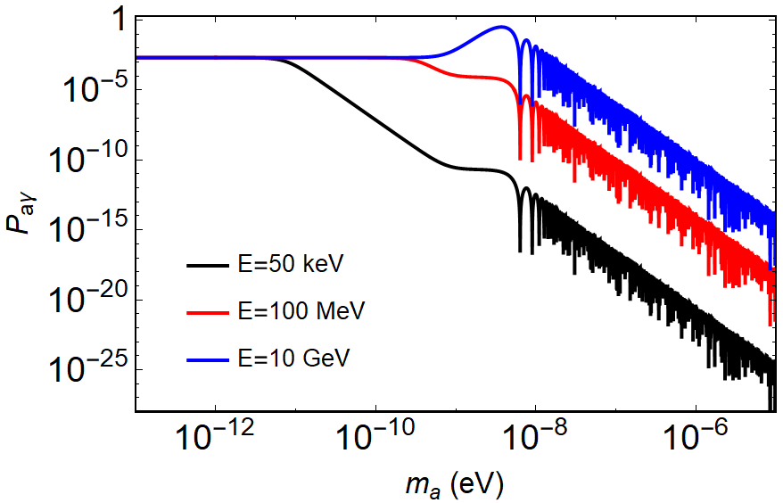
As obvious from Eq. (19), for a massless ALP the condition $\Phi\ll 1$ is satisfied for distances $r\lesssim 20$ kpc at energies of $E\sim 10$ keV. A finite ALP mass may spoil this condition. The exact mass threshold for this to happen depends on the distance $r$, and on the ALP energy. In particular, high energy ALPs may be correlated on a larger distance and for larger masses. On the other hand, for large ALP masses $\Phi\gg 1$ and the oscillation probability acquires a dependence on the energy and decreases rapidly with the axion mass, $P_{a\gamma}\propto m_{a}^{-4}$, as evident in Figure 1, where we show the behavior of the conversion probability $P_{a\gamma}$ for a source at distance $r=1$ kpc for a value of the regular magnetic field $B_{\rm reg}=3$ $\mu$G in function of the ALP mass $m_{a}$. In the Figure, we fixed the axion coupling to $g_{a\gamma}=10^{-11}\rm GeV^{-1}$ and take three representative ALP energies: $E=50$ keV (black curve), representative of the typical energy of ALPs emitted from a red supergiant star during its late evolutionary stages [20]; $E=100$ MeV (red curve), representative of the energies of ALPs emitted from supernova explosions [23]; and $E=10$ GeV (blue curve), representative of gamma-rays from galactic pulsars [9].

A realistic description of the photon-ALP oscillation in the Galactic magnetic field requires a model for the magnetic field with both regular and turbulent components. The most commonly adopted model for the regular component is the Jansson-Farrar model [24] (see, e.g., Refs. [35, 7, 9]), though the Pshirkov model [25] is a common alternative choice.

The small-scale turbulent field is less well known. It is usually assumed to follow a power law with a certain outer scale, where energy is injected, which then cascades down to smaller turbulent scales until energy dissipates at the dissipation scale [36]. The strength of this random magnetic field component can be estimated from rotation measure fluctuations, combined with an estimate of the thermal electron density, giving a ratio of random to regular magnetic field components of $\lesssim 1$ [38, 37]. This value is compatible with the predictions of large-scale magnetic field models that include the turbulent magnetic field as a free parameter [39].

Concerning the correlation length, Ref. [29] found a large $l_{\rm corr}\sim 100$ pc, using structure functions of rotation measures and averaging over large parts of the sky. Ref. [30] confirmed this large outer scale for interarm regions in the Galactic plane; however, they found a much smaller outer scale $\sim 10$ pc in the spiral arms. Also, arrival anisotropies in TeV cosmic-ray nuclei can be best explained by a turbulent magnetic interstellar medium on a maximum scale of about $\sim 1$ pc [31]. More recently, an upper limit of $\sim 20$ pc for the outer scale of the magnetic interstellar turbulence toward the Fan region has been found in Ref. [28] by measuring with LOFAR the fluctuations in the diffuse synchrotron emission.

We now consider different representative situations showing the impact of the turbulent component of the Galactic magnetic field on the ALP-photon conversion. For definiteness, we take a source at a distance $r=1$ kpc. There are several Galactic ALP sources, such as red supergiants, within a radius of ${\mathcal{O}}(1)$ kpc [40]. ALPs produced in these sources would propagate in a magnetized medium where they can convert into photons. In our examples below, we take the regular component of the magnetic field to be uniform on such a short length scales. In any case, scales of 1 kpc are not resolved in large scales simulations. On the other hand, for the turbulent component we assume a correlation length $l_{\rm corr}=10$ pc. The choice of a very short correlation length is conservative since, as we shall see below, increasing $l_{\rm corr}$ enhances the effect of the turbulent field on the conversion probability [Cf. Eq. (20)]. In the description of the turbulent Galactic magnetic field we adopt a simplified approach, assuming it along a given line-of-sight as a network of domains with a fixed correlation length $l_{\rm corr}=10$ pc. ¹¹ 1 A more refined characterization of turbulent $B$-fields in ALP conversions can be found in [41]. Finally, we fix $B_{\rm reg}=3$ $\mu$G and assume a turbulent component with a root-mean-square (rms) amplitude $B_{\rm rms}=1$ $\mu$G [24]. As a representative situation, we consider ALPs with coupling $g_{a\gamma}=10^{-11}$ GeV^-1, a value slightly below the current experimental and astrophysical bounds, and energy $E=50$ keV. We will vary the ALP mass in order to probe different cases of ALP oscillation length.

In the conditions described above, an ALP mass above about 1 neV corresponds to a correlation length $l_{\rm osc}=2\pi/\Delta_{\rm osc}\simeq 4$ pc $\ll l_{\rm corr}$. The associated conversion probability, in this case, is negligibly small, $P_{a\gamma}\lesssim 10^{-9}$. Therefore, we will ignore this case hereafter and limit ourselves to situations in which $l_{\rm osc}>l_{\rm corr}$. Within this hypothesis, we can show that when the conversion probability is small, the effects induced by the turbulent magnetic field can be evaluated analytically. As shown in Appendix A, the average probability over all possible field configurations in function of the distance $r$ from the source is remarkably simple,

where $P_{a\gamma}^{(0)}(r)$ is the probability assuming only a regular magnetic field. We remark that Eq. (20) is valid also when the regular magnetic field is not homogeneous, as long as $P_{a\gamma}\ll 1$. This is the typical situation for conversions in the Milky Way, assuming allowed values for the ALP-photon coupling and a realistic magnetic field. When $P_{a\gamma}\sim O(1)$ the previous approach is no longer valid and in general we have to resort to a Monte Carlo simulation. However, in the hypothesis of $\delta$–correlated perturbations it is possible to modify the evolution equations in order to calculate arbitrary moments of the variable $P_{a\gamma}$. Although this situation is outside the scope of this work, for completeness we treat this case in Appendix B.

A full derivation of Eq. (20) is provided in Appendix A. However, it is easy to recognize the validity of this result also using very simple arguments. Assuming $l_{\rm corr}\ll l_{\rm osc}$, it is possible to express the average conversion probability on a given magnetic domain as $P_{a\gamma,\rm turb}^{(0)}\simeq(g_{a\gamma}B_{\rm rms}l_{\rm cell}/2)^{2}=(g_{a\gamma}B_{\rm rms}l_{\rm corr})^{2}$, where the size of a single magnetic domain is given by $l_{\rm cell}=2l_{\rm corr}$ (see Appendix A). Since the photons travel $N=r/l_{\rm corr}$ magnetic configurations, the incoherent total conversion probability on the turbulent configuration is given by $P_{a\gamma,\rm turb}\simeq NP_{a\gamma,\rm turb}^{(0)}=g_{a\gamma}^{2}B_{\rm rms}^{2}l_{\rm corr}r$ (see also Ref. [3]).

We notice that since the turbulent field has a random configuration, $P_{a\gamma}$ is a random variable itself. In the hypothesis that the turbulent magnetic field has a gaussian distribution, $f(\widetilde{B}_{x,y})\propto\exp(-\widetilde{B}_{x,y}^{2}/2B_{\rm rms}^{2})$, we can calculate the probability density function $F(P_{a\gamma})$ in the limit in which the diagonal terms in the Hamiltonian in Eq. (6) are small (see Appendix A). If this condition is not fulfilled, it is very difficult to obtain a closed form for the probability distribution function (p.d.f.) but it is still possible to get handy formulas for the calculation of the momenta of $P_{a\gamma}$. In particular one can obtain the second momentum of $P_{a\gamma}$ [Eq. (35)] and thus the standard deviation of the distribution, $\sigma(r)=[\langle P^{2}_{a\gamma}(r)\rangle-\langle P_{a\gamma}(r)\rangle^{2}]^{1/2}$. In Appendix A we compare our analytical results with a numerical simulation to show the agreement between the two approaches.

In Figs. 2, 4, and 5, we show examples of the ALP-photon oscillation probability in three different scenarios. In particular, in Figure 2 we consider the case $m_{a}=10^{-10}$ eV, corresponding to $l_{\rm osc}\simeq 400$ pc. The red curve is the conversion probability for a purely regular $B$-field. The black curve is the average probability in presence of regular plus turbulent fields, calculated using Eq. (20). The gray band represents the “$1\sigma$” dispersion around the average represented by the grey-band. Here, by “$1\sigma$” we mean the standard deviation around the mean value. This cannot immediately translate into a definite confidence level since the p.d.f. is not in general a gaussian. We see that the $1\sigma$ dispersion in the probability induced by the turbulent component is seizable, producing variations up to $\sim$50% with respect to the average. For the purpose of illustration, with the blue line we show the conversion probability for one representative random realization of the magnetic field. The realization of the magnetic field used to draw this representative case is plotted in Fig. 3. We observe that the behavior of $P_{a\gamma}(r)$ for a single realization is in general irregular, depending on the configuration of the field. In particular, the chosen realization for $r\gtrsim 0.5$ kpc gives a conversion probability smaller than the purely regular field. In general, some realizations of the turbulent field could result in a conversion probability smaller than the one obtained with a purely regular field. However, the average probability is always larger compared to a regular field.

In Figure 4, we consider an ALP with mass $m_{a}=10^{-11}$ eV, which implies $l_{\rm osc}\simeq 35$ kpc. This case corresponds to an energy-independent oscillation probability. As expected, the conversion probability induced by the regular component of the magnetic field scales as $r^{2}$. The effect of the turbulent component is the spread of the $P_{a\gamma}$ around the mean. Although on average the effect is very small, for many realizations the difference with the regular case can exceed up to 10% within $1\sigma$. Since in this case $\Delta_{\rm pl},\Delta_{a}\ll\Delta_{a\gamma}$ we can use the analytic expression for the p.d.f. [Eq. (53) in Appendix A]. For example, we estimate that at distance $r=1$ kpc about the 31.7% of the values of $P_{a\gamma}$ lie outside the $\pm 1\sigma$ band.

Finally, in order to isolate the role of the turbulent field, in Fig. 5 we consider the same case of Fig. 4, but assuming only the turbulent component of the magnetic field. We show the average and the $1\sigma$ band for a pure turbulent field with $B_{\rm rms}=1$ $\mu$G. In this case, as expected from Eq. (20), we see that $\langle P_{a\gamma}(r)\rangle$ grows linearly (at least until $\langle P_{a\gamma}\rangle\ll 1$). Also in the last two cases in blue we draw a representative conversion probability curves, using the same realizations drawn in Fig. 3.

References

- [1] A. De Angelis, O. Mansutti and M. Roncadelli, “Axion-Like Particles, Cosmic Magnetic Fields and Gamma-Ray Astrophysics,” Phys. Lett. B 659, 847-855 (2008) doi:10.1016/j.physletb.2007.12.012 [arXiv:0707.2695 [astro-ph]].
- [2] A. Mirizzi, G. G. Raffelt and P. D. Serpico, “Photon-axion conversion in intergalactic magnetic fields and cosmological consequences,” Lect. Notes Phys. 741, 115-134 (2008) doi:10.1007/978-3-540-73518-2_7 [arXiv:astro-ph/0607415 [astro-ph]].
- [3] A. Mirizzi, G. G. Raffelt and P. D. Serpico, “Signatures of Axion-Like Particles in the Spectra of TeV Gamma-Ray Sources,” Phys. Rev. D 76, 023001 (2007) doi:10.1103/PhysRevD.76.023001 [arXiv:0704.3044 [astro-ph]].
- [4] D. Hooper and P. D. Serpico, “Detecting Axion-Like Particles With Gamma Ray Telescopes,” Phys. Rev. Lett. 99, 231102 (2007) doi:10.1103/PhysRevLett.99.231102 [arXiv:0706.3203 [hep-ph]].
- [5] M. Simet, D. Hooper and P. D. Serpico, “The Milky Way as a Kiloparsec-Scale Axionscope,” Phys. Rev. D 77, 063001 (2008) doi:10.1103/PhysRevD.77.063001 [arXiv:0712.2825 [astro-ph]].
- [6] F. V. Day, “Cosmic axion background propagation in galaxies,” Phys. Lett. B 753, 600-611 (2016) doi:10.1016/j.physletb.2015.12.058 [arXiv:1506.05334 [hep-ph]].
- [7] G. Galanti, F. Tavecchio, M. Roncadelli and C. Evoli, “Blazar VHE spectral alterations induced by photon–ALP oscillations,” Mon. Not. Roy. Astron. Soc. 487, no.1, 123-132 (2019) doi:10.1093/mnras/stz1144 [arXiv:1811.03548 [astro-ph.HE]].
- [8] M. Berg, J. P. Conlon, F. Day, N. Jennings, S. Krippendorf, A. J. Powell and M. Rummel, “Constraints on Axion-Like Particles from X-ray Observations of NGC1275,” Astrophys. J. 847, no.2, 101 (2017) doi:10.3847/1538-4357/aa8b16 [arXiv:1605.01043 [astro-ph.HE]].
- [9] J. Majumdar, F. Calore and D. Horns, “Search for gamma-ray spectral modulations in Galactic pulsars,” JCAP 04, 048 (2018) doi:10.1088/1475-7516/2018/04/048 [arXiv:1801.08813 [hep-ph]].
- [10] M. C. D. Marsh, J. H. Matthews, C. Reynolds and P. Carenza, “Relativistic axion-photon conversion in astrophysical magnetic fields,” to be published
- [11] M. Meyer, D. Horns and M. Raue, “First lower limits on the photon-axion-like particle coupling from very high energy gamma-ray observations,” Phys. Rev. D 87, no.3, 035027 (2013) doi:10.1103/PhysRevD.87.035027 [arXiv:1302.1208 [astro-ph.HE]].
- [12] R. Buehler, G. Gallardo, G. Maier, A. Domínguez, M. López and M. Meyer, “Search for the imprint of axion-like particles in the highest-energy photons of hard -ray blazars,” JCAP 09, 027 (2020) doi:10.1088/1475-7516/2020/09/027 [arXiv:2004.09396 [astro-ph.HE]].
- [13] D. Montanino, F. Vazza, A. Mirizzi and M. Viel, “Enhancing the Spectral Hardening of Cosmic TeV Photons by Mixing with Axionlike Particles in the Magnetized Cosmic Web,” Phys. Rev. Lett. 119, no.10, 101101 (2017) doi:10.1103/PhysRevLett.119.101101 [arXiv:1703.07314 [astro-ph.HE]].
- [14] N. Bassan, A. Mirizzi and M. Roncadelli, “Axion-like particle effects on the polarization of cosmic high-energy gamma sources,” JCAP 05, 010 (2010) doi:10.1088/1475-7516/2010/05/010 [arXiv:1001.5267 [astro-ph.HE]].
- [15] O. Mena, S. Razzaque and F. Villaescusa-Navarro, “Signatures of photon and axion-like particle mixing in the gamma-ray burst jet,” JCAP 02, 030 (2011) doi:10.1088/1475-7516/2011/02/030 [arXiv:1101.1903 [astro-ph.HE]].
- [16] C. Csaki, N. Kaloper and J. Terning, “Dimming supernovae without cosmic acceleration,” Phys. Rev. Lett. 88, 161302 (2002) doi:10.1103/PhysRevLett.88.161302 [arXiv:hep-ph/0111311 [hep-ph]].
- [17] A. Mirizzi, G. G. Raffelt and P. D. Serpico, “Photon-axion conversion as a mechanism for supernova dimming: Limits from CMB spectral distortion,” Phys. Rev. D 72, 023501 (2005) doi:10.1103/PhysRevD.72.023501 [arXiv:astro-ph/0506078 [astro-ph]].
- [18] A. Avgoustidis, C. Burrage, J. Redondo, L. Verde and R. Jimenez, “Constraints on cosmic opacity and beyond the standard model physics from cosmological distance measurements,” JCAP 10, 024 (2010) doi:10.1088/1475-7516/2010/10/024 [arXiv:1004.2053 [astro-ph.CO]].
- [19] E. D. Carlson, “Pseudoscalar conversion and X-rays from stars,” Phys. Lett. B 344, 245-251 (1995) doi:10.1016/0370-2693(94)01529-L
- [20] M. Xiao, K. M. Perez, M. Giannotti, O. Straniero, A. Mirizzi, B. W. Grefenstette, B. M. Roach and M. Nynka, “Constraints on Axionlike Particles from a Hard X-Ray Observation of Betelgeuse,” Phys. Rev. Lett. 126, no.3, 031101 (2021) doi:10.1103/PhysRevLett.126.031101 [arXiv:2009.09059 [astro-ph.HE]].
- [21] J. W. Brockway, E. D. Carlson and G. G. Raffelt, “SN1987A gamma-ray limits on the conversion of pseudoscalars,” Phys. Lett. B 383, 439-443 (1996) doi:10.1016/0370-2693(96)00778-2 [arXiv:astro-ph/9605197 [astro-ph]].
- [22] J. A. Grifols, E. Masso and R. Toldra, “Gamma-rays from SN1987A due to pseudoscalar conversion,” Phys. Rev. Lett. 77, 2372-2375 (1996) doi:10.1103/PhysRevLett.77.2372 [arXiv:astro-ph/9606028 [astro-ph]].
- [23] A. Payez, C. Evoli, T. Fischer, M. Giannotti, A. Mirizzi and A. Ringwald, “Revisiting the SN1987A gamma-ray limit on ultralight axion-like particles,” JCAP 02, 006 (2015) doi:10.1088/1475-7516/2015/02/006 [arXiv:1410.3747 [astro-ph.HE]].
- [24] R. Jansson and G. R. Farrar, “A New Model of the Galactic Magnetic Field,” Astrophys. J. 757, 14 (2012) doi:10.1088/0004-637X/757/1/14 [arXiv:1204.3662 [astro-ph.GA]].
- [25] M. S. Pshirkov, P. G. Tinyakov, P. P. Kronberg and K. J. Newton-McGee, “Deriving global structure of the Galactic Magnetic Field from Faraday Rotation Measures of extragalactic sources,” Astrophys. J. 738, 192 (2011) doi:10.1088/0004-637X/738/2/192 [arXiv:1103.0814 [astro-ph.GA]].
- [26] M. Haverkorn, “Magnetic Fields in the Milky Way”. In: Lazarian A., de Gouveia Dal Pino E., Melioli C. (eds) Magnetic Fields in Diffuse Media, Astrophysics and Space Science Library, vol. 407. Springer, Berlin, Heidelberg doi:10.1007/978-3-662-44625-6_17
- [27] W. Reich, E. Fuerst, P. Reich, et al. 2004, proceedings of “The Magnetized Interstellar Medium,” (Antalya, Turkey, September 8-12, 2003), ed. B. Uyaniker, W. Reich, & R. Wielebinski, 45-50
- [28] M. Iacobelli, M. Haverkorn, E. Orrú, R. F. Pizzo, J. Anderson, R. Beck, M. R. Bell, A. Bonafede, K. Chyzy and R. J. Dettmar, et al. “Studying Galactic interstellar turbulence through fluctuations in synchrotron emission: First LOFAR Galactic foreground detection,” Astron. Astrophys. 558, A72 (2013) doi:10.1051/0004-6361/201322013 [arXiv:1308.2804 [astro-ph.GA]].
- [29] H. Ohno and S. Shibata, “The random magnetic field in the Galaxy,” Mon. Not. Roy. Astron. Soc. 262, no. 4, 953-962 (1993) doi:10.1093/mnras/262.4.953
- [30] M. Haverkorn, J. C. Brown, B. M. Gaensler and N. M. McClure-Griffiths, “The outer scale of turbulence in the magneto-ionized Galactic interstellar medium,” Astrophys. J. 680, 362 (2008) doi:10.1086/587165 [arXiv:0802.2740 [astro-ph]].
- [31] M. A. Malkov, P. H. Diamond, L. ’. C. Drury and R. Z. Sagdeev, “Probing Nearby CR Accelerators and ISM Turbulence with Milagro Hot Spots,” Astrophys. J. 721, 750-761 (2010) doi:10.1088/0004-637X/721/1/750 [arXiv:1005.1312 [astro-ph.GA]].
- [32] G. Raffelt and L. Stodolsky, “Mixing of the Photon with Low Mass Particles,” Phys. Rev. D 37, 1237 (1988) doi:10.1103/PhysRevD.37.1237
- [33] V. Anastassopoulos et al. [CAST], “New CAST Limit on the Axion-Photon Interaction,” Nature Phys. 13, 584-590 (2017) doi:10.1038/nphys4109 [arXiv:1705.02290 [hep-ex]].
- [34] R.C. Almy, D. McCammon, S.W. Digel, L. Bronfman and J. May, “Distance Limits on the Bright X-Ray Emission Toward the Galactic Center: Evidence for a Very Hot Interstellar Medium in the Galactic X-Ray Bulge,” Astrophys. J. 545, 290-300 (2000) doi:10.1086/317768
- [35] D. Horns, L. Maccione, M. Meyer, A. Mirizzi, D. Montanino and M. Roncadelli, “Hardening of TeV gamma spectrum of AGNs in galaxy clusters by conversions of photons into axion-like particles,” Phys. Rev. D 86 (2012), 075024 doi:10.1103/PhysRevD.86.075024 [arXiv:1207.0776 [astro-ph.HE]].
- [36] C. Evoli, P. Blasi, G. Morlino and R. Aloisio, “Origin of the Cosmic Ray Galactic Halo Driven by Advected Turbulence and Self-Generated Waves,” Phys. Rev. Lett. 121, no.2, 021102 (2018) doi:10.1103/PhysRevLett.121.021102 [arXiv:1806.04153 [astro-ph.HE]].
- [37] D. H. F. M. Schnitzeler, P. Katgert and A. G. de Bruyn, “WSRT Faraday tomography of the Galactic ISM at lambda~0.86 m,” Astron. Astrophys. 471, L21 (2007) doi:10.1051/0004-6361:20077635 [arXiv:0706.2548 [astro-ph]].
- [38] M. Haverkorn, P. Katgert and A. G. de Bruyn, “Properties of the warm magnetized ISM, as inferred from WSRT polarimetric imaging,” Astron. Astrophys. 427, 169-177 (2004) doi:10.1051/0004-6361:200400042 [arXiv:astro-ph/0406557 [astro-ph]].
- [39] T. R. Jaffe, J. P. Leahy, A. J. Banday, S. M. Leach, S. R. Lowe and A. Wilkinson, “Modelling the Galactic Magnetic Field on the Plane in 2D,” Mon. Not. Roy. Astron. Soc. 401, 1013 (2010) doi:10.1111/j.1365-2966.2009.15745.x [arXiv:0907.3994 [astro-ph.GA]].
- [40] M. Mukhopadhyay, C. Lunardini, F. X. Timmes and K. Zuber, “Presupernova neutrinos: directional sensitivity and prospects for progenitor identification,” Astrophys. J. 899, no.2, 153 (2020) doi:10.3847/1538-4357/ab99a6 [arXiv:2004.02045 [astro-ph.HE]].
- [41] A. Kartavtsev, G. Raffelt and H. Vogel, “Extragalactic photon-ALP conversion at CTA energies,” JCAP 01 (2017), 024 doi:10.1088/1475-7516/2017/01/024 [arXiv:1611.04526 [astro-ph.HE]].
- [42] https://earth.esa.int/web/eoportal/satellite-missions/n/nustar
- [43] F. Calore, P. Carenza, M. Giannotti, J. Jaeckel and A. Mirizzi, “Bounds on axionlike particles from the diffuse supernova flux,” Phys. Rev. D 102, no.12, 123005 (2020) doi:10.1103/PhysRevD.102.123005 [arXiv:2008.11741 [hep-ph]].
- [44] A. Mezzacappa and S. W. Bruenn, “A numerical method for solving the neutrino Boltzmann equation coupled to spherically symmetric stellar core collapse,” Astrophys. J. 405, 669-684 (1993) doi:10.1086/172395
- [45] M. Liebendoerfer, O. E. B. Messer, A. Mezzacappa, S. W. Bruenn, C. Y. Cardall and F. K. Thielemann, “A Finite difference representation of neutrino radiation hydrodynamics for spherically symmetric general relativistic supernova simulations,” Astrophys. J. Suppl. 150, 263-316 (2004) doi:10.1086/380191 [arXiv:astro-ph/0207036 [astro-ph]].
- [46] M. Meyer, M. Giannotti, A. Mirizzi, J. Conrad and M. A. Sánchez-Conde, “Fermi Large Area Telescope as a Galactic Supernovae Axionscope,” Phys. Rev. Lett. 118, no.1, 011103 (2017) doi:10.1103/PhysRevLett.118.011103 [arXiv:1609.02350 [astro-ph.HE]].
- [47] https://fermi.gsfc.nasa.gov/science/instruments/table1-1.html
- [48] A. De Angelis et al. [e-ASTROGAM], “Science with e-ASTROGAM: A space mission for MeV–GeV gamma-ray astrophysics,” JHEAp 19, 1-106 (2018) doi:10.1016/j.jheap.2018.07.001 [arXiv:1711.01265 [astro-ph.HE]].
- [49] R. Caputo et al. [AMEGO], “All-sky Medium Energy Gamma-ray Observatory: Exploring the Extreme Multimessenger Universe,” [arXiv:1907.07558 [astro-ph.IM]].
- [50] Z. Q. Xia, C. Zhang, Y. F. Liang, L. Feng, Q. Yuan, Y. Z. Fan and J. Wu, “Searching for spectral oscillations due to photon-axionlike particle conversion using the Fermi-LAT observations of bright supernova remnants,” Phys. Rev. D 97, no.6, 063003 (2018) doi:10.1103/PhysRevD.97.063003 [arXiv:1801.01646 [astro-ph.HE]].
- [51] G. A. Pallathadka, F. Calore, P. Carenza, M. Giannotti, D. Horns, J. Majumdar, A. Mirizzi, A. Ringwald, A. Sokolov and F. Stief, “Reconciling hints on axion-like-particles from high-energy gamma rays with stellar bounds,” [arXiv:2008.08100 [hep-ph]].
- [52] M. Libanov and S. Troitsky, “On the impact of magnetic-field models in galaxy clusters on constraints on axion-like particles from the lack of irregularities in high-energy spectra of astrophysical sources,” Phys. Lett. B 802 (2020), 135252 doi:10.1016/j.physletb.2020.135252 [arXiv:1908.03084 [astro-ph.HE]].
- [53] M. Meyer, D. Montanino and J. Conrad, “On detecting oscillations of gamma rays into axion-like particles in turbulent and coherent magnetic fields,” JCAP 1409 (2014) 003 doi:10.1088/1475-7516/2014/09/003 [arXiv:1406.5972 [astro-ph.HE]].
- [54] G. E. P. Box and M. E. Muller, “A note on the generation of random normal deviates”, The Annals of Mathematical Statistics 29 (1958), no. 2 610–611.
- [55] A. G. Redfield, “The Theory of Relaxation Processes”, Advances in Magnetic and Optical Resonance, Academic Press, Volume 1, 1965, ISBN 9781483231143.
- [56] F. N. Loreti and A. B. Balantekin, “Neutrino oscillations in noisy media,” Phys. Rev. D 50 (1994), 4762-4770 doi:10.1103/PhysRevD.50.4762 [arXiv:nucl-th/9406003 [nucl-th]].
- [57] R. B. Sidje, “Expokit: A Software Package for Computing Matrix Exponentials,” ACM Trans. Math. Softw. 24, 130 (1998). Software package available at www.maths.uq.edu.au/expokit/
- [58] G. Barenboim and N. E. Mavromatos, “CPT violating decoherence and LSND: A Possible window to Planck scale physics,” JHEP 01 (2005), 034 doi:10.1088/1126-6708/2005/01/034 [arXiv:hep-ph/0404014 [hep-ph]].