Re-entrant superconductivity through a quantum Lifshitz transition in twisted trilayer graphene
Abstract
A series of recent experiments have demonstrated robust superconductivity in magic-angle twisted trilayer graphene (TTG). In particular, a recent work by Cao et al. (arxiv:2103.12083) studies the behavior of the superconductor in an in-plane magnetic field and an out-of-plane displacement field, finding that the superconductor is unlikely to have purely spin-singlet pairing. This work also finds that at high magnetic fields and a smaller range of dopings and displacement fields, it undergoes a transition to a distinct field-induced superconducting state. Inspired by these results, we develop an understanding of superconductivity in TTG using a combination of phenomenological reasoning and microscopic theory. We describe the role that that an in-plane field plays in TTG, and use this understanding to argue that the re-entrant transition may be associated with a quantum Lifshitz phase transition, with the high-field phase possessing finite-momentum pairing. We argue that the superconductor is likely to involve a superposition of singlet and triplet pairing, and describe the structure of the normal state. We also draw lessons for twisted bilayer graphene (TBG), and explain the differences in the phenomenology with TTG despite their close microscopic relationship. We propose that a singlet-triplet superposition is realized in the TBG superconductor as well, and that the correlated insulator may be a time reversal protected topological insulator obtained through spontaneous spin symmetry breaking.
I Introduction
A remarkable series of developments have brought two-dimensional graphene-based Moire materials to the spotlight of condensed matter physics. Many of these systems host a fascinating array of strongly correlated insulating and magnetic states Cao et al. 2018a; Chen et al. 2019; Sharpe et al. 2019; Chen et al. 2020a; Serlin et al. 2020; Zondiner et al. 2020; Saito et al. 2020; Saito et al. 2021; Wu et al. 2021; Chen et al. 2020b; Cao et al. 2020; Rozen et al. 2020; Zhou et al. 2021; Balents et al. 2020; Andrei et al. 2021, and twisted bilayer graphene (TBG) in particular displays robust unconventional superconductivity Liu et al. 2020; Lu et al. 2019; Yankowitz et al. 2019; Cao et al. 2018b; Arora et al. 2020. Recently, another Moire system, twisted trilayer graphene (TTG), was also predicted and subsequently found to exhibit robust superconductivity Khalaf et al. 2019; Li et al. 2019; Hao et al. 2021; Park et al. 2021a. A very recent work Cao et al. 2021 studies superconductivity in near-magic angle TTG in the presence of an in-plane magnetic field and an out-of-plane electric displacement field , and finds some strking phenomena as we review below. In the present paper we will synthesize the existing experimental results into a coherent theoretical picture of the superconductivity in TTG. We will explain the differences with the closely related twisted bilayer graphene (TBG), and will show how comparing phenomena in TTG and TBG can give us important clues to understand both systems.
We begin with a discussion of some of the salient experimental results on superconductivity in near magic-angle TTG Hao et al. 2021; Park et al. 2021a; Cao et al. 2021. Our focus will be on the robust superconductivity found for moire lattice fillings in the range .
- 1.
The ‘normal’ state out of which the superconductivity emerges has a carrier density that is set by the deviation from . This normal state has a Landau fan degeneracy of , rather than the -fold degeneracy naively expected on the basis of the available flavor degrees of freedom (spin and valley). Furthermore the strength of the superconductivity does not seem to correlate with the single particle density of states inferred from indirect measurements.
- 2.
The superconductivity occurs even without the external perturbations of the perpendicular displacement field or the in-plane magnetic field . Weak and have contrasting effects on the superconductivity - the former enhances it while the latter suppresses it. Strikingly Ref. Cao et al. 2021 finds that the superconducting state in a range of fillings survives in fields far in excess of the Pauli limit, suggesting that the pairing is not spin-singlet in nature. This behavior is also notably different from that seen in TBG, where the superconductivity is suppressed by a roughly at the Pauli limit.
- 3.
Near optimal doping and displacement field strength, the superconductivity is seen to exhibit a “re-entrant” phenomenon at large magnetic fields, with a phase transition that separates two distinct superconductors occurring at a field T. Interestingly, while the temperature at which superconductivity occurs goes to zero at , the temperature at which the resistance reaches a fixed fraction of its normal-state value is smooth across the transition, and decreases monotonically with .
In what follows, by combining the input from experiments with a Ginzburg-Landau analysis, together with the insights from simple microscopic theory, we will provide an understanding of these phenomena, and make predictions for future experiments. We will be naturally led to the conclusion that the pairing in the superconductor is neither spin singlet nor spin triplet, but rather a linear combination of the two. We examine the role that the and fields play in the physics of TTG, and highlight differences with TBG. This will enable an explanation of the striking differences in the stability of the superconductor to in-plane fields in the two systems. We propose that interpreting the re-entrant transition as arising from a Lifshitz critical point, where one or both components of the superfluid stiffness vanish and where the pairing in the high-field phase occurs at finite momentum, is particularly natural in light of the existing experimental data.
Along the way we also discuss the nature of the normal state near filling . We propose that at the ground state is a time reversal protected topological insulator (obtained through spontaneous spin symmetry breaking) coexisting with the massless Dirac fermions corresponding to a decoupled graphene sector.
At , the physics of TTG is very closely related to that of TBG Khalaf et al. 2019, as will be reviewed shortly. This leads us to propose that our conclusions about the nature of the pairing in the superconductor and the nature of the normal state at hold in TBG as well, with minor but important modifications. This allows for experiments in TTG, which in some respects are easier to interpret than those in TBG, to improve our understanding about both systems.
What we do not attempt to do in this paper is a full-blown microscopic theory of TTG superconductivity. The questions we are interested in involve very complicated strongly interacting systems where the understanding from theory is only partially complete. Thus we view our semi-phenomenological approach as the safest way of proceeding, since it allows us to avoid committing to any particular calculational schemes of specific microscopic models, both of which come with uncertainties at present.
II Basic model
Let us first review the basic theoretical description of TTG Khalaf et al. 2019. We will take the graphene layers to lie normal to the axis, and will gauge-fix the in-plane vector potential so that on layer , where with the interlayer separation. The displacement field enters the Hamiltonian through an onsite potential of on layers 1, 2, and 3 respectively, where . The exact proportionality constant depends on details of how the screening works, and will not be important for the present discussion.
To proceed it is most convenient to work in a basis of fields that have definite eigenvalues under the action of mirror Khalaf et al. 2019; Calugaru et al. 2021, which exchanges layers 1 and 3 and which is a symmetry when . In the basis with , where annihilate electrons on layer , the single-particle Hamiltonian is
| (1) |
where the Zeeman energy . Here is the monolayer Dirac velocity, is the hopping matrix familiar from the bilayer problem (see appendix E), , and we have used the notation , with Pauli matrices for valley, sublattice, and physical spin, respectively. For simplicity we have also ignored a rotation of the on layers 1 and 3 by the twist angle, since its effects are small Bistritzer and MacDonald 2011; Tarnopolsky et al. 2019. Typical orbital magnetic energies are on the order of a few meV, with Zeeman energies smaller by a factor of .
We note in passing that the Hamiltonian (1) is the correct starting point only when the top and bottom graphene layers are not displaced relative to one another in the xy plane. A nonzero relative displacement breaks mirror symmetry, and can have strong effects on the flat band physics Lei et al. 2020. However, a vanishing relative displacement is likely to be favored energetically Carr et al. 2020, and at the data of Ref. Cao et al. 2021 appear to be mirror-symmetric to a good approximation. We will therefore set in the following.
From (1), we see that in the absence of or , decouples into a TBG Hamiltonian for the mirror-even fields , which form a set of flat bands near the magic angle, together with a decoupled Dirac cone formed by the mirror-odd field Khalaf et al. 2019. Given that plays a crucial role in the observed superconductivity, the physics of the superconductivity is likely to be closely related to effects caused by the mirror-odd Dirac cone.
The mirror symmetry of the Hamiltonian has other important consequences for how affects the single-particle physics, as both and are odd under mirror (here denotes the orbital field). In particular, at the spectrum at each momentum must be an even function of . This means that unlike in TBG, at there will be no field-induced de-pairing of intervalley Cooper pairs due to misalignement of the Fermi surfaces in the two valleys Cao et al. 2020, as here the single-particle energy satisfies even when . The fact that the leading effects are at order also means that at small , the orbital effects of the magnetic field are rather weak. Diagonalizing at realistic values of , one finds two Dirac cones at the moire point at energies separated by an amount which increases with , as well as a Dirac cone located very near the point. Details on the single-particle physics can be found in appendix E.
One observation from Ref. Cao et al. 2021 is that despite the sensitivity of the observed superconductivity to and , superconductivity near optimal doping is seen even when . Therefore the mirror-even fermions must be superconducting on their own, independent of their coupling to the mirror-odd .11 1 One possibility is that dissipation from the fermions promotes superconductivity in the mirror-even sector, along the lines of the mechanism in Ref. Vishwanath et al. 2004a. In what follows we will however assume that the dominant effects of the fermions arise from the terms written in (2). We are therefore prompted to analyze the system by considering the Lagrangian (suppressing all indices)
| (2) | ||||
where is the superconducting order parameter and is some unknown Lagrangian capturing the physics of the superconductor, together with the Zeeman energy for the mirror-even fermions. The term proportional to arises from a mean-field decoupling of an interaction of the form . Such a term does not arise from a standard density-density interaction, but as it is allowed by symmetries we will keep it.
Importantly, the modifications to the superconductivity by can be reliably addressed by integrating out the fermions perturbatively, as it is only through the mixing with these fermions that these perturbations have any effect.
III The normal state near
Before attempting to obtain an effective action for by integrating out the fermions in (2), it is helpful to think about constraints on the matrix structure of by considering the likely nature of the normal state near . As we will see, known properties of the superconductor will help us place nontrivial constraints on the nature of the normal state. Because this discussion takes place at , we may temporarily ignore the mirror-odd fermions: this is because in this limit the leading coupling of the fermions to the mirror-even fields vanishes,22 2 In principle there are also higher-body interactions between the fermions and the mirror even sector — in what follows we will assume that these interactions do not qualitatively change the nature of the normal state, which seems reasonable on account of the low density of the fermions. rendering the problem equivalent to that of TBG Khalaf et al. 2019. This simplication is quite useful, as it allows us to draw on insights gained in the study of TBG. Aspects of the physics particular to TTG will arise when we turn on nonzero , which is discussed in the following sections.
Existing experiments on TTG Park et al. 2021a; Hao et al. 2021 indicate that the normal state at is likely highly resistive (and presumably would be insulating in the absence of the Dirac cone). Additionally, the doped state at is seen to possess a Landau level degeneracy reduced from that of the charge neutrality point by a factor of two. The simplest way to produce a ground state in accordance with these observations is to polarize a flavor, and then to open an interaction-induced gap in the remaining polarized subspace. We will be making the assumption that the superconductor pairs fields related by time reversal, implying that both valleys participate in the superconducting state. We will also be assuming (at least at small ) that the superconductor inherits the flavor polarization of the normal state. This implies that the normal state is not valley polarized, and in what follows we will assume that the polarized flavor is spin. Spin polarization here means that the ground state is spin-valley locked (SVL), with the spins in a given valley fixed to lie along some (valley-dependent) direction.
The assumption of spin-valley locking is reasonable from a theoretical point of view, as polarizing spin (as opposed to valley) allows the system to take advantage of the intervalley Hund’s coupling. This assumption is also motivated by experiment, as SVL allows the superconductor to achieve the strong Pauli limit violation observed in Ref. Cao et al. 2021.
The simplest way to open up a gap is to give some fermion bilinear a nonzero expectation value, where the indices run over the states in the low-energy SVL subspace. To determine what we should take for the form of , we will borrow results from the strong-coupling picture proposed for twisted bilayer graphene in Refs. Bultinck et al. 2020; Khalaf et al. 2020a. In this picture, the four flat bands in the SVL subspace can be labeled as and , where denote normalized spinors determining the directions along which the spins are locked in the , valleys respectively, and where is the sublattice index (which is a good index for the flat bands in the strong-coupling limit Bultinck et al. 2020). The first set of two bands has Chern number , and the second set of two have . The strong-coupling analysis indicates that must mix the two valleys, and must be proportional to in sublattice space, this being the only matrix structure which allows the ordered state at to completely fill two of the Chern bands and minimize the kinetic and potential energy in the strong-coupling limit (see Bultinck et al. 2020 for the full logic). Any which fulfills these properties and survives projection onto the occupied SVL subspace may be written as
| (3) |
where the matrix written out explicitly is in valley space and where the phase is arbitrary. A nonzero expectation value for breaks time reversal symmetry unless the spins in each valley are antiferromagnetically aligned.
At zero magnetic field, the relative orientation of is dictated by the sign of the intervalley Hund’s coupling . The sign of is not known a priori, and is determined by a delicate competition between various effects, e.g. Coulomb interactions and coupling to phonons Chatterjee et al. 2020. However, as we will see momentarily, the fact that the superconductor seen in experiment has a nonzero BKT transition temperature at zero field means that must favor antiferromagnetic alignment of the spins in the two valleys (for the case without SVL, see appendix B). For definiteness we will take the zero-field normal state to have , so that
| (4) |
There are two important things to note about . The first is that it is invariant under time reversal symmetry, as the spins are aligned antiferromagnetically. Given that the zero-field state at contains two filled bands with Chern numbers , this antiferromagnetic SVL state is, remarkably, therefore a topological insulator protected by the unbroken and symmetries.33 3 This should be contrasted with the analysis of the spinless model of Ref. Bultinck et al. 2020 where the proposed state is also topological, protected by and a symmetry which combines time reversal with a valley rotation. Such a symmetry is not sufficient to protect gapless edge states as the valley symmetry is broken at the edge. In contrast the spinful state discussed in this paper will have protected edge states. The second is that rotations of the spin about act on in the same way as the group of opposite phase rotations in the two valleys. Therefore the order parameter manifold of the insulator is . As there are no skyrmions in this state (only vortices), complicating a skyrmion-driven mechanism for superconductivity along the lines of that proposed in Refs Khalaf et al. 2020a; Chatterjee et al. 2020 (although depending on the strength of , a description in terms of skyrmions that exist at intermediate scales may still be useful).
IV Ginzburg-Landau theory
We now turn to discussing the general features that we expect any Ginzburg-Landau (GL) free energy for the observed superconductor should satisfy.
As mentioned above, we are operating under the assumption that is off-diagonal in the valley index. Interaction effects similar to those mentioned above then mandate Khalaf et al. 2020a; Khalaf et al. 2020b; Lee et al. 2019 that be proportional to the identity in sublattice space (so that pairing takes place between opposite Chern sectors). For the present discussion, we will further assume that over the full temperature range of interest, the spin-valley locking which likely occurs in the normal state is inherited by the superconductor (the case where this assumption is relaxed is treated in appendix B).
With these assumptions, we may write the order parameter as
| (5) | ||||
where the matrix on the first line is in valley space, and the four-vector has components
| (6) |
Note that in writing down this form for the order parameter, we have assumed that the pairing occurs in an even angular momentum channel. None of the analysis to follow is affected by this choice, and odd angular momentum pairing can be treated simply by interchanging and in the above expression for .
A general expression for the GL free energy in the SVL subspace can be written in terms of and the vectors as
| (7) | ||||
where , the coefficient determines whether the spins in each valley prefer to align ferromagnetically or antiferromagnetically, and where all of the coefficients in the above expression contain implicit dependence on and , with this dependence determined from the Lagrangian (2) (to be discussed shortly).
Suppose first that , so that the spins in each valley prefer to align ferromagnetically along some direction , which is chosen spontaneously when . The order parameter is then invariant under the combined action of gauge rotations and spin rotations about . The order parameter manifold for the zero-field superconductor is therefore . Consequently, this phase does not have a finite- BKT transition at . Furthermore, since this phase only has vortices, the critical current in zero field vanishes Cornfeld et al. 2020, and when the free energy of this state decreases linearly in the presence of a small in-plane field. All of these features are in disagreement with experiment.
When on the other hand, the spins align antiferromagnetically in the plane normal to the field direction at small , and then gradually cant to point along the field at larger (see Fig. 1). This canting process happens without breaking apart the Cooper pair, allowing the superconductor to survive at fields above the Pauli limit. Unlike in the case, the free energy and condensate fraction do not evolve linearly with near (appendix B contains the details). Furthermore, since is invariant under spin rotations about the ordering direction when , the order parameter manfiold in the zero field limit is . Then there are vortices with integer-valued charge that cost logarithmic energy, leading to a nonzero at zero field. All of these features are in agreement with experiment.
We are therefore forced to conclude that the zero-field superconductor favors antiferromagnetic alignment. This provides the justification for our assumption in the previous section that the normal state has antiferromagnetic spin-valley locking (see Ref. Khalaf et al. 2020b for a similar argument).
It now remains to understand the mechanism producing the re-entrant phenomenon seen in experiment, as well as to understand the dependence of and on the applied fields. This can be done by understanding the dependence of the coefficients appearing in the free energy, which we now turn to discussing.
V Quantum Lifshitz criticality and finite-momentum pairing
As mentioned in the introduction, a particularly noteworthy aspect of the experiment is that decreases more or less smoothly all the way until superconductivity is completely killed, while shows non-monotonic behavior in Cao et al. 2021.44 4 We note however that a subsequent experiment Liu et al. 2021 did not find evidence for a non-monotonic . The temperature is set by the condensate fraction . By contrast, is set by the superfluid stiffness , viz. the coefficient of the term in the free energy, where is the phase mode of .
A natural explanation for the observed re-entrant phenomenon is therefore that decreases monotonically with by a factor , while decreases faster with , and goes to zero when , where the phase transition occurs (see the schematic phase diagram in Fig. 1.) When , becomes negative.
The IR physics of the superconductor is dominated by the phase mode ,55 5 For nonzero field strengths which are not strong enough to fully lock the spins along , there is an additional neutral spin mode coming from spin rotations about the field direction. It however is not important for the following discussion, and will be ignored. with a Lagrangian capturing the essential physics being
| (8) |
where is included for stability. The proposed re-entrant transition is a Lifshitz point, where vanishes.
Whether or not a Lifshitz transition can occur is determined by the field dependence of the coefficients in the GL free energy, which can be calculated by integrating out the fermions in the Lagrangian (2). The important point here is that only enter (2) in the coupling of to , and since is simply a free Dirac cone, the field dependence of the terms in the free energy can be calculated in a perturbatively controlled way. We find that to quadratic order in and , the coupling between the fermions result in the parameter and the stiffness appearing in the free energy (7) being renormalized by amounts
| (9) | ||||
where are all positive coefficients, whose detailed form is not important for the present discussion. The upshot is that (at least at small fields), the displacement field tends to promote superconductivity, while the orbital field leads to a suppression in both the condensate fraction and spin stiffness. The fact that the orbital and displacement fields have opposite effects on the superconductor (at least at small ) originates from the different ways in which they couple the fermions together. Importantly, this is exactly the behavior seen in experiment, with the superconductivity strengthened (suppressed) with increasing (increasing ), at least in the range of displacement fields for which the re-entrant transition occurs. The details of the calculation leading to (9) are standard, and are relegated to appendix A. A rough estimate of the critical in-plane field for the superconductor at in terms of the mircoscopic parameters which enter the coefficients appearing in (9) is given in appendix D. Our estimate is of the same order of magnitude as the critical field observed in experiment and we will be satisfied with this consistency check, leaving a more detailed calculation to future work.
This dependence of on is precisely of the form required for the proposed Lifshitz transition to work, with the Lifshitz transition occurring if is large enough to drive to zero before . Furthermore, the fact that the condensate fraction increases with to quadratic order provides an explanation for why, at moderate values of , the superconductivity is seen to be stronger with increasing . That the re-entrant transition occurs only at moderate values of can be understood in the same way, as the Lifshitz transition can only occur if remains nonzero at the field strength where is driven to zero. In this scenario, at small values of it is which goes to zero first with increasing , while at larger values of it is that goes to zero first.
Note that due to the rotational symmetry breaking by the in-plane field, it is possible that the stiffnesses along and normal to the field direction differ, so that
| (10) |
where () denote derivatives along (normal to) the field direction. One could therefore consider a situation in which only one of is driven to zero at the Lifshitz transition. However, the isotropic case where go to zero simultaneously seems more likely to be realized. Indeed, consider the case where only one component vanishes at . The critical point is an anisotropic Lifshitz model. In appendix C we show that this model orders at , and displays QLRO up to some non-universal nonzero temperature. Thus in this scenario we would not expect the observed to go all the way to zero at (although the temperature at which the anisotropic model looses QLRO is likely very small, and may well be below the current experimental resolution).
On the other hand consider the isotropic case, where both and vanish at . In this case the critical point has no QLRO at any temperature Ghaemi et al. 2005, so that at the critical point, as seems to be the case experimentally. Another reason for favoring the isotropic case is that to leading order in , and are renormalized by the same amount. Our prior is therefore that near the critical point, to a good approximation. However, it may well be the case that in narrow field regimes only one of is negative, possibly explaining the rather broad nature of the transition and the observed small pockets of potentially distinct superconducting phases Cao et al. 2021.
On the other side of the Lifshitz phase transition, the pairing occurs at finite momentum. Note that this scenario is very different in spirit to the usual FFLO mechanism Fulde and Ferrell 1964; Larkin and Ovchinnikov 1965, since the latter relies on Pauli pair breaking being the dominant mechanism to suppress superconductivity. This is opposite to case of the superconductor currently under consideration, which strongly violates the Pauli limit and in which the main effects of the field are orbital in nature. Because the present mechanism differs from that of FFLO, in order to minimize the condensation energy the order parameter will presumably live at a single nonzero wavevector , so that that has a spatially uniform magnitude.
The first indications from Ref. Cao et al. 2021 are that the re-entrant transition is first order. As written down in (8) the transition is second order, but in general it may be driven first order by other higher-order terms not included in (8) Fradkin et al. 2004; Vishwanath et al. 2004b. One example is the term , which is marginally relevant if Vishwanath et al. 2004b.66 6 The cubic term also renders the critical point first order, but is not invariant under the symmetry of the theory, which sends and Po et al. 2018. Also note that nonzero permits us to write down other relevant cubic terms like (with the included to preserve mirror symmetry). These terms however are not generated in the context of our model, as the effects of the orbital coupling only enter at order (see appendix A).
VI Lessons for TBG
As was emphasized above, in the absence of external fields the fermions decouple form the mirror-even sector, rendering the system nearly identical to TBG together with a decoupled Dirac fermion. In particular, this means that the physics of the superconductor and the normal state near are likely to be the same in both TBG and TTG. As we have argued that at the superconductor near in TTG has antiferromagnetic spin-valley locking and pairing which involves a superposition of spin singlet and spin triplet, the same should be true in TBG (see also Ref. Khalaf et al. 2020b) .
How should we reconcile this conclusion with the striking differences between TBG and TTG in the presence of a nonzero in-plane magnetic field? In TBG, the critical in-plane field in the superconducting state at optimal filling is Cao et al. 2018b, which is much smaller than in TTG, and is much closer to the Pauli limit. Since we claim that the pairing in TBG also involves a combination of spin singlet and spin triplet, the comparatively small value of in TBG cannot be due to Zeeman effects. Instead, the critical field is set by orbital effects. Indeed, unlike in TTG the single-particle energies in TBG do not satisfy in a nonzero orbital field, allowing orbital pair-breaking effects to produce a relatively lower value for Cao et al. 2020. The suppression of superconductivity at roughly the Pauli limit in an in-plane field was interpreted early on as evidence for a spin singlet superconductor. This interpretation was first called into question by the observation that the in-plane critical field is strongly angle dependent Cao et al. 2020. Such angle dependence cannot arise from Zeeman effects. Within the present picture the superconductor is a superposition of singlet and triplet, its suppression by an in-plane field is entirely orbital, and the rough agreement with the Pauli limit is a coincidence coming from the rough equality of the orbital Zeeman g-factor and the spin g-factor.
Turning to the normal state of TBG, a striking consequence of the antiferromagneic spin-valley locking is that, within the strong coupling theory, the correlated insulating state at is an interaction-driven TI. This state will have time reversal protected edge states which will be interesting to look for in future experiments.
Finally, a puzzle which we do not resolve is that the insulating state at in TBG is also suppressed by an in-plane magnetic field Cao et al. 2018a; Yankowitz et al. 2019 (while in TTG the suppression seems to be mostly absent Liu et al. 2021). There are conflicting reports Yankowitz et al. 2019; Wu et al. 2021; Park et al. 2021b on the details of how the insulating gap in TBG evolves with a field (linear in some experiments, quadratic in others), and we leave the understanding of this phenomenon to the future.
VII Discussion and Summary
In this paper we have used a combination of phenomenological and microscopic theoretical reasoning to build a coherent picture of the superconductivity and related phenomena in TTG. We argued that the superconducting state is a superposition of spin singlet and spin triplet pairings. We showed how this explains the contrasting effects of small displacement and fields, even though both break mirror symmetry. We also showed that the mirror symmetry explains the striking difference between the stability of TTG and TBG superconductors to in-plane fields despite their close microscopic relationship. We proposed that the re-entrant superconductivity recently observed in twisted trilayer graphene Cao et al. 2021 can be explained by a spin-valley locked superconductor which undergoes a quantum Lifshitz transition into a finite-momentum pairing state in the presence of an in-plane magnetic field. The close relationship between TBG and TTG when the displacement field and magnetic field are turned off enables insights from the bilayer system to contribute to the study of the trilayer case, and vice versa. One consequence of this is our conclusion that the normal state near in twisted bilayer graphene may be a TI.
A possible test of our proposal for the re-entrant superconductor in TTG is to measure the Josephson current between two neighboring TTG regions maintained at different displacement fields. Due to the dependence of on the displacement field , it is possible to tune between the low-field and high-field phases in constant magnetic field, by varying alone. Therefore one could imagine engineering a Josephson tunneling experiment between the low- and high-field superconducting states simply by varying the applied electric field in space. If the high-field state has finite-momentum pairing, the Josephson current should vanish, due to the spatially oscillating phase of the high-field phase’s order parameter Yang and Agterberg 2000. Of course, a vanishing current could also occur by virtue of the high- and low-field phases having different pairing symmetries. However, if the pair momentum in the high-field state is a continuously varying function of (as in our analysis), the Josephson current between two high-field superconducting regions maintained at different displacement fields should also vanish, providing a stronger test of the proposed Lifshitz scenario.
In the case which the high-field state is obtained through an (anisotropic) Lifshitz transition, one could also simply measure whether or not the critical current is direction-dependent, as near the phase transition the critical current should be highly direction-dependent (see appendix C).
Finally, the conclusion that the normal state near is a TI is also interesting from an experimental perspective, as it will have symmetry protected gapless edge states in a single domain sample. In TTG, this TI coexists with the massless Dirac fermions of the mirror-odd sector. Complications caused by the mirror-odd Dirac cone could potentially be avoided in a setup where the sample edge is mirror symmetric and electrical contact is made only with the middle layer, enabling the transport properties of the mirror-even sector to be isolated. It may also be interesting to study the effects of induced spin orbit coupling in this system, along the lines of Ref. Lin et al. 2021, to explicitly lock in the symmetry breaking leading to the TI sector.
The proposed TI at may be more readily accessible to experiments in TBG, where there are no extra gapless mirror-odd fermions.
Acknowledgements
We thank Yuan Cao, Jane Park, and Pablo Jarillo-Herrero for extensive conversations about their experiments. EL is supported by the Fannie and John Hertz Foundation and the NDSEG fellowship. TS was supported by US Department of Energy grant DE- SC0008739, and partially through a Simons Investigator Award from the Simons Foundation. This work was also partly supported by the Simons Collaboration on Ultra-Quantum Matter, which is a grant from the Simons Foundation (651440, TS).
Appendix A Microscopic derivation of the terms in the Ginzburg-Landau free energy
In this appendix we describe how the and dependence of the coefficients appearing in GL free energy (68) can be obtained microscopically, starting from the Lagrangian
| (11) | ||||
where as in the main text (recall that ), and where contains the physics of the mirror-even flat band fermions and the superconductor. As in the main text, we will assume even angular momentum pairing and write the order parameter as
| (12) |
The fact that is proportional to the identity in the sublattice index and off diagonal in the valley index is important, with this matrix structure being responsible for several important minus signs in what follows. However, the assumption of even angular momentum pairing is not important, and odd angular momentum pairing can be treated simply by exchanging and in the above expression.
In what follows we will treat the mirror-even fermions by assuming that they form a flavor unpolarized Fermi liquid. Situations in which flavor polarization occurs can be easily dealt with by inserting appropriate projectors into traces. In particular, if the polarized flavor is spin, with the spins being locked to valley (which as we have argued in the main text is likely the case relevant for experiment), the effects of the polarization only enter when dealing with the Zeeman couplings, and can be dealt with in the manner described near (57).
A.1 Orbital effects
We begin by examining the orbital effects of the magnetic field. The only place where the orbital coupling enters into the above Lagrangian is in the term, which couples the symmetric and antisymmetric sectors. This allows the effects of to be treated within a controlled perturbative expansion.
Integrating out produces the term
| (13) |
where is the propagator. Since we are remaining largely agnostic about the physics of the symmetric flat bands, we do not know what looks like, other than that it involves s on the off-diagonals. In what follows we will simply assume that the most important effects of can be captured by the term
| (14) |
where is a constant. Here and below, the notation is to be read as “ is a term appearing in ”.
We now integrate out and examine the structure of the resulting terms generated in the effective action for . Thus the remaining task is to compute the functional determinant
| (15) | ||||
where
| (16) |
and where the particle / hole Greens functions are
| (17) |
We will assume that integrating out leaves the fermions as continuing to be well-described by a Dirac cone, albeit one with a renormalized (possibly anisotropic) Dirac velocity and a nonzero chemical potential. Therefore we take to be (ignoring for now the Zeeman coupling)
| (18) |
so that
| (19) |
In the following we will use the notation
| (20) |
with containing powers of . We will first turn to examining the quadratic piece .
A.1.1 Quadratic terms
We will work at for now, as the effects of a small nonzero do not qualitatively modify the structure or field dependence of the terms that are generated. We will also only focus on the behavior of in the zero-frequency limit, by taking . After re-scaling momenta by , , we have
| (21) |
To perform the trace, we can use the explicit expression for to write
| (22) | ||||
where in this appendix , we have defined
| (23) |
and have used as well as
| (24) | ||||
The fact that and enter in with opposite signs is important for the physics of the Lifshitz transition, and is a consequence of the fact that pairs opposite valleys, and hence anticommutes with the contained in . Note that this physics is independent of our assumption of even angular momentum pairing, since it only relies on the fact that is off-diagonal in the valley index.
Performing the trace, we then find
| (25) |
Introducing a Feynman parameter (integrated from 0 to 1),
| (26) |
where .
Doing the sum over Matsubara frequencies,
| (27) |
The exact expression for this integral is not so important for the present purposes, as we are mostly just interested in the signs of the order terms. We find
| (28) |
where are positive (temperature-dependent) coefficients. Selecting out the contribution which depends on the displacement and magnetic fields and by using the definition of , and dropping terms of order , we then have
| (29) |
A.1.2 Quartic terms
We now examine how the orbital field affects the the quartic terms in the GL free energy. Using , we have (now restricting to zero momentum transfer)
| (30) | ||||
A.1.3 Summary
To understand the consequences of the terms derived so far, consider the simplified free energy , where the phase stiffness is related to as . The effects derived in (29), (30) lead to renormalizations of by amounts
| (31) | ||||
where we have assumed for simplicity.
The condensate fraction is renormalized by
| (32) |
where are the values of in the absence of any coupling between the mirror-even and mirror-odd fermions.
The exact field dependence of depends on the magnitude of and the sign of , which are not things that can be derived microscopically within the current approach. First consider the case where is small enough so that terms of order may be dropped compared to those of order , and the contribution from the term can be ignored. This very well may be the case microscopically, as the interaction which produces the term does not appear in the (presumably dominant) density-density interaction (see the discussion following (2)). In this case we have
| (33) |
Therefore the displacement field increases the condensate fraction, while the magnetic field decreases it. The same dependence also holds for . Note in particular that in this limit, the condensate fraction is unchanged by the magnetic field when (at least to order ), implying that to this order the critical in-plane magnetic field is infinite.
When is not small compared to , it is possible to engineer a situation where the behavior of the condensate fraction is reversed from the discussion above (provided that ). This however can be ruled out from experiment, given that the condensate fraction is seen to increase with at (at least for the range of displacement fields we are interested in). Therefore in this case the leading shifts of the condensate fraction and of are both proportional to , with positive constants of proportionality. Note that this gives a finite value of even when , as in experiment. This could either be because the experimental system has a nonzero (though possibly small) value of , or because the mirror symmetry is not perfect.
Summarizing, we conclude that the displacement field and (orbital) magnetic field have opposite effects: the displacement field increases both the condensate fraction and the superfluid stiffness, while the magnetic field decreases both the condensate fraction and the superfluid stiffness. Because and are renormalized by different amounts, it is reasonable to consider a scenario where the superfluid stiffness goes to zero with increasing before the condensate fraction does.
A.2 Zeeman effects
We now turn to examining contributions to the effective action for arising from the Zeeman coupling of the magnetic field to the microscopic fermions. These contributions come from the term
| (34) |
where for brevity we have defined .
A.2.1 Response from a Fermi liquid
Modeling the mirror-even fermions as a Fermi liquid as described at the beginning of this appendix, we can incorporate the Zeeman effects they induce by using the propagators
| (35) | ||||
where is the energy measured relative to the Fermi energy. This then provides the term
| (36) | ||||
At linear order in , this gives the contribution
| (37) | ||||
where we shifted the momentum integration and used that the response will only be a function of , so that can be replaced with . Evaluating the trace, we find
| (38) |
where as before , and where
| (39) |
For simplicity we will only explicitly evaluate the term. In the limit where we can replace with , this term vanishes due to particle-hole symmetry about the Fermi level. The leading contribution is thus proportional to Sugiyama and Ohmi 1995, giving
| (40) |
Due to the smallness of in a generic Fermi liquid scenario, this term would normally be neglected. However, it is possible that the displacement field modifies the density of states significantly enough to make this term important at moderate .
Before moving on, we note that the above term was derived by performing an expansion in powers of , using the normal state form of the fermion propagators. In the limit where , we should instead perform an expansion about the superconductor. In this case the term simply vanishes, as there is no magnetization for the field to couple to.
Now we look at effects from (36) which enter at order . Using
| (41) |
the contribution at order is
| (42) | ||||
where the second term in the first line comes from the expansion of the s in the denominators of the propagators, and we have again used that the response is only a function of when going to the second line.
The general expressions that appear after doing the frequency sum are rather complicated. For our purposes it suffices to expand in , and write
| (43) |
where the are all positive functions of , with all but vanishing in the limit where we may perform the integrals as .
A.2.2 Response from a Dirac cone
We now compute the Zeeman effects induced by the mirror-odd Dirac fermion (these are expected to be smaller, but we include the discussion for completeness). To do this, we need to compute the propagator for in the absence of hybridization with . To this end, consider the matrix
| (44) |
One can show that the inverse is
| (45) |
If we apply this to the case of , we expand to order and get
| (46) | ||||
where . We then use these propagators to integrate out and compute the resulting terms in the effective action for , following the same approach as when considering orbital effects.
The contribution linear in vanishes if due to particle-hole symmetry, but is nonzero otherwise. To leading (linear) order in ,
| (47) | ||||
where is a positive constant.
Contributions at order give the term (now dropping the chemical potential for simplicity)
| (48) | ||||
Evaluating the integrals gives
| (49) |
where as usual are positive (temperature dependent) constants.
Appendix B Details on the Ginzburg-Landau theory
In this section we detail the phases described by the Ginzburg-Landau theory discussed in the main text. See Scheurer and Samajdar 2020 for a similar analysis in a more general context.
B.1 Fully spin-valley locked limit
We will first consider the case where the spin is fully locked to valley, so that the order parameter is allowed to be nonzero only in a subset of the Hilbert space.
As was discussed above near (71), in the case of full SVL, we have and may write the order parameter as
| (50) |
where as before , the matrix written out explicitly is in valley space, and where are normalized spinors which determine the directions along which the spins in the valleys are polarized.
By decomposing the outer products appearing in in terms of Pauli matrices, we may write (assuming even angular momentum pairing for concreteness, as in the main text)
| (51) | ||||
where the four-vector is defined in terms of , and has components
| (52) |
where we have defined the adjoint spinor77 7 The adjoint of a given spinor is obtained by inverting the spinor through the Bloch sphere and changing the handedness used to define its overall phase. In terms of the Euler angle parametrization (53) the adjoint can be obtained by by sending
| (54) |
In what follows it will be helpful to define, for any spinor , the three-vector
| (55) |
Taking the adjoint in the manner above simply reverses the direction of the 3-vector, so that . This notation lets us write the magnitudes of and as
| (56) | ||||
The norm of the full vector is thus , giving as required. Also as expected for a spin-polarized state, we see that the weight of the triplet part is always nonzero, being minimal for antiferromagnetic alignment between the valleys and maximal for ferromagnetic alignment, with the opposite being true for the weight of the singlet part .
When deriving the coefficients in the GL free energy microscopically, SVL can be taken into account simply by replacing the particle and hole propagators by
| (57) |
where we have defined the projector
| (58) |
with the in valley space. Note that satisfies
| (59) |
The form of terms not involving the Zeeman coupling of the magnetic field are not modified by the projection. For terms involving the Zeeman coupling, we simply make the replacement
| (60) |
The structure of the Zeeman terms quadratic in the magnetic field are determined by following the analysis of appendix A, and using the traces
| (61) | ||||
For example, for a spin-valley locked Fermi liquid, the contributions to the free energy from the Zeeman couplings are, to quadratic order in and ,
| (62) |
where is small in and (see appendix A). As expected, we may avoid Pauli suppression of the pairing either by having the spins in each valley align in the plane normal to , or by having the two spins ferromagnetically align along , both of which prevent pair-breaking by the field from occurring.
The free energy in general may be written as a function of as (ignoring derivatives of for simplicity)
| (63) |
where the coefficient determines whether the spins in each valley prefer to align ferromagnetically or antiferromagnetically. The explicit dependence arises from the Zeeman coupling terms, while the orbital effects of the field provide implicit dependence of the various coefficients on in the manner described in appendix A.
As discussed in the main text, the system observed in experiments likely has . When , the minimum of occurs for . is now invariant under rotations about , and hence the order parameter manifold is .
Now we will examine what happens to this state at nonzero . Taking to lie along in spin space, upon minimizing we find
| (64) |
where represents a rotation by an arbitrary angle about , and where
| (65) |
Thus for the spins are partially magnetized and there is an s worth of degenerate minima, and as in the partially polarized phase of the following subsection the order parameter manifold is . For the spins are ferromagnetically aligned and fully magnetized, and the order parameter manifold is . Given this solution for , the magnitude of the order parameter is consequently determined to be
| (66) |
The condensate fraction and its first derivative with respect to are continuous across the transition into the high-field ferromagnetic state, and , implying that unlike in the non-locked case to be discussed in the next subsection, will not increase linearly with at small .


Figure 2 shows the condensate fraction (left panel) and magnetization (center panel) for a typical choice of parameters (here is small enough so that the system never reaches the fully magnetized regime). The right panel is the same as the left, but shows the BKT temperature after taking into account orbital effects which suppress .
B.2 No spin-valley locking
Now we consider the slightly simpler case in which there is no spin-valley locking (SVL), with the order parameter allowed to have components in the entire fermionic Hilbert space. This discussion will therefore only be germane for the problem considered in this paper at values of and / or large enough to eliminate any SVL which occurs in the normal state near .
We start by breaking the order parameter up into triplet and singlet parts as
| (67) |
where is a complex four-vector. Up to quartic order in the order parameter, the free energy can be written as
| (68) | ||||
where we have used the standard notation . As usual, the terms which depend explicitly on the magnetic field arise from Zeeman effects, while orbital effects are responsible for giving the remaining coefficients implicit dependence on .
When minimizing in the presence of of the couplings to the magnetic field, it is often helpful to write the vector in terms of components which diagonalize the coupling Kawaguchi and Ueda 2012. Taking the magnetic field to point in the direction in spin space, this is done through the unitary transformation
| (69) |
In this representation, the and components of the free energy are now
| (70) | ||||
The effects of the term can be understood as a way of softly implementing SVL. Indeed, if we write the order parameter as
| (71) |
(where the 2 matrix is in valley space) we see that we may write
| (72) |
Therefore large positive enforces that the determinant of vanish. In this case we may write
| (73) |
for two spinors , which have the interpretation as the directions along which the spins in the valleys are polarized. For simplicity of the analytical results, and because the fully spin-valley locked case was discussed in the last subsection, in what follows we will simply set .
Extremizing the free energy for uniform solutions then gives
| (74) | ||||
One can show that when , which is the case we are interested in, when the global minima of the free energy always have , while when we have spin symmetry and may fix without loss of generality. Setting then, when we just have to solve
| (75) | ||||
where
| (76) |
and88 8 When the RHS of (77) becomes negative, the minimum of has . The solutions in this case are obtained simply by replacing with .
| (77) |
There are now two types of solutions. The first is with or , corresponding to fully spin-polarized triplets. Choosing , the favored solution will be the one with . This gives the fully polarized solution
| (78) |
where () shifts under gauge transformations ( spin rotations about ). This order parameter is therefore invariant under combined and rotations. As a result, when the order parameter manifold is Cornfeld et al. 2020, since the subgroup can be absorbed into the part. As discussed in the main text, this means that at there are only vortices and that , which is incompatible with experiment. When the order parameter manifold is instead , so that vortices (and a nonzero ) occur at finite fields.
When both and are nonzero, we find the partially polarized solution
| (79) |
which is only a solution provided that the field is less than the critical value , where
| (80) |
which only implicitly determines due to the implicit dependence of the coefficients on the RHS. When , is invariant under spin rotations about , but unlike the fully polarized case the only rotation which acts in the same way as a gauge transformation is a spin flip, which acts in the same way as a gauge rotation by . The order parameter manifold when is therefore . Since , the phase has vortices and a nonzero Mukerjee et al. 2006. When , the order parameter manifold is instead .
When the fully polarized solution is favored regardless of , while when the partially polarized solution is favored as long as . The transition at occurs when vortices in the spin mode condense, and is of BKT type within the context of the present discussion. Since we know from experiments that the low-field phase is not fully polarized, we may therefore assume in what follows.


Figure 3 shows the condensate fraction and magnetization for a typical choice of parameters. Panels a) and b) show the condensate fraction and magnetization, with the lines drawn at the locations of the BKT transitions separating the various phases. Panel c) shows where the transitions occur upon accounting for a further suppression of the stiffness by orbital effects (see appendix A), with the Lifshitz transition occurring at the field where first goes to zero.
Note that for any nonzero magnetic field, the transition into the fully polarized state always occurs before superconductivity is killed altogether ( in figure 3). This is because the fully polarized state is favored by a term which is linear in (the term), while the partially polarized state is favored by a term quadratic in (the term); hence when is small the fully polarized solution always wins. This means that in the limit, near the boundary of the superconducting dome the superconductor will always be in the fully polarized phase, regardless of the strength of the magnetic field. As a result, increases linearly with at small , by an amount which is small in . Since in the context of magic-angle TTG we expect to be small, especially so at small (again, see appendix A), this may or may not be incompatible with experiment.
Appendix C Nature of the Lifshitz critical points
In this appendix we elaborate on the nature of the Lifshitz critical points discussed in section V. Throughout we will write down free energies which involve only the phase mode , with the fluctuations in the spin part of the order parameter ignored on grounds that they flow to zero coupling in the IR.
C.0.1 Isotropic case
We first review the isotropic case, where the Lagrangian at the critical point contains no quadratic derivative terms:
| (81) |
A complete discussion of the finite-temperature physics of this model can be found in Ghaemi et al. 2005; here we will review the results of Ghaemi et al. 2005 which are relevant for the present discussion.
The spatial correlator calculated from (81) is logarithmically divergent in the IR at , and the model has QLRO. At nonzero the divergence is power law, so that the correlation functions of are ultra short-ranged. This latter fact does not mean that the model is necessarily disordered at all however, since as stressed in Ghaemi et al. 2005 irrelevant terms will generate a nonzero stiffness (i.e, a nonzero term), allowing the correlators to decay as power laws at .
Accounting for these effects at is done by starting instead with the Lagrangian
| (82) |
where the marginally irrelevant term is responsible for generating a nonzero stiffness at , and is a counterterm ensuring that the renormalized stiffness vanish at .
The renormalized stiffness can be computed within the framework of an RPA (large-) approximation. In this approximation, is given by the bare value in addition to a contribution coming from a geometric sum of 1-loop diagrams involving the interaction. Writing the renormalized propagator as , we have
| (83) | ||||
where we have used the requirement that at to solve for .
The value of determines by way of the Kosterlitz-Thouless criterion . Since in the present case at low , there will not be a BKT transition at finite , and the theory is disordered for all non-zero temperatures Ghaemi et al. 2005.
C.0.2 Anisotropic case
Let us now apply a similar analysis to the anisotropic case, where only one component of the stiffness vanishes at the critical point. At , we may work with the Lagrangian
| (85) |
where is needed for stability. We take to be dimensionless, with the dimensionful factor of out front having dimensions of . At zero temperature the correlator along e.g. the direction goes as
| (86) |
which is IR finite. The theory therefore orders at , unlike in the isotropic case Pisarski and Tsvelik 2021. However, like the isotropic case, the finite- correlator calculated using the above Lagrangian (85) has a power-law divergence in the system size: for example, at large ,
| (87) |
which diverges as , with the system size.
As in the isotropic case, this divergence does not rule out the existence of a finite- phase with QLRO, as we must account for the presence of other terms which generate a nonzero component of the stiffness at .
At , the correct starting point is therefore instead, analogously to (82),
| (88) |
The renormalized stiffness can be computed using the same 1-loop diagram as before. We have
| (89) | ||||
Assuming , we can ignore the dependence of the third term in the integral. We then solve for , finding
| (90) |
where . At small we indeed have , justifying our earlier assumption. Note that unlike in the isotropic case, here we are not in the upper critical dimension of the theory, and the term which generates is not marginal. Therefore there is no logarithmic dependence of on , and the dependence of on the value of can not a priori be neglected at low .
In the anisotropic case, the stiffness which determines the location of a possible BKT transition is set by . Since , will always be larger than at low enough , meaning that there will always be a finite-temperature BKT transition. Explicitly, in the present approximation the transition occurs at
| (91) |
The value of is of course non-universal, and depending on the microscopics may very well be small enough to be essentially indistinguishable in experiments from zero.
C.0.3 Critical currents
In this section we compute the critical current in the region of parameter space near the Lifshitz transition.
First consider the normal phase where the pairing occurs at zero momentum. In this case we may examine the free energy density
| (92) |
where . To determine the critical current, we follow the standard procedure Tinkham 2004 of Legendre transforming to a thermodynamic potential which is a function of the current , satisfying (working in units where )
| (93) |
Therefore
| (94) |
Minimizing over gives
| (95) |
Maximizing the RHS, we then see that the critical currents along the and directions are given by
| (96) |
Now we consider a situation which favors finite-momentum pairing along the direction. We consider the free energy density
| (97) |
with . We then consider an FF state, with
| (98) |
and assume that varies on scales much longer than . We can then consider the approximate free energy
| (99) |
Repeating the same steps as above leads to critical currents of
| (100) |
Consider finally the scenario where both quadratic derivatives in the free energy density have negative coefficients Buzdin et al. 2007; Samokhin and Truong 2017, with
| (101) |
with all coefficients except positive. Consider again an FF state , with finite momentum in the direction. Assuming and making the same approximations as above, this leads to the critical currents
| (102) |
Appendix D Estimate of the in-plane critical field
In this appendix we provide a crude estimate of the critical in-plane field of the superconductor at zero displacement field and optimal doping. Given the phenomenological nature of our analysis and the fact that may very well not be small enough for leading-order perturbation theory in to be reliable, this calculation is not meant to be taken as a sharp prediction — rather it is meant simply as a consistency check to make sure that our proposal is not grossly incompatible with experiment.
From equation (31) of appendix A, the stiffness at zero displacement field and small is given by99 9 Note that we are ignoring contributions to the stiffness which arise from Zeeman effects. Within the framework of appendix A, Zeeman effects in the mirror-even sector do not contribute to the stiffness at leading order, while contributions from the mirror-odd sector are small (being suppressed by a factor of ), and will be ignored. (assuming for simplicity that the velocity of the mirror-odd Dirac cone after integrating out the mirror-even fermions is isotropic and equal to the monolayer value of )
| (103) |
where are terms higher order in , nm is the interlayer separation, is the phase stiffness, and where the definitions of will be recapitulated shortly. Estimating the zero-field stiffness as where K Cao et al. 2021 is the zero-field transition temperature, we have
| (104) |
where the energy scale is defined as
| (105) |
We now need to estimate the quantities appearing in .
The coupling is associated with the pairing terms for the mirror-odd fermions that arise upon integrating out the mirror-even sector (see (14)), and has dimension of inverse energy squared. While we are not in a position to calculate exactly, on general grounds we expect , where is the Fermi energy of the mirror-even bands which become superconducting. is not known exactly and its determination depends on knowledge of what happens to the correlated insulator at upon hole doping, but a value in the ballpark of a few tens of mev seems appropriate.
can be read off from an expansion of (27), giving
| (106) |
where is integrated from 0 to 1 and . For the present purposes of estimating , we will take in the above.
The appropriate value to take for (equal to the superconducting gap in our mean-field treatment) is not currently known experimentally. We will leave as a free parameter for now, and note only that due to the strong-coupling nature of the problem and the energy scales involved, a value of mev does not seem unreasonable.
Finally, we need to estimate the dimensionless parameter , which appears in our Lagrangian as and originates from a mean-field decoupling of interactions of the form (all indices suppressed). These interaction only conserve the number of mirror-even and mirror-odd fermions modulo 2, and they do not appear directly in the regular density-density interaction, as the total fermion density is which separately conserves the number of mirror-even and mirror-odd fermions. These interactions furthermore do not arise at first order upon projecting the density-density interaction to the active bands, since at the form factors of the active bands do not mix the mirror-even and mirror-odd sectors (by symmetry). Therefore after projecting the interaction to the active bands, can only arise from an interaction corresponding to a second-order process involving tunneling to remote bands. The strength of these higher-order interactions is roughly , where is the gap to the remote bands and is the Coulomb interaction strength; is accordingly . Estimating mev (with the relative dielectric constant ) and mev (based on a naive reading of the band structure Khalaf et al. 2019; Fischer et al. 2021 gives .
With the above estimates in hand, we may plug in numbers and write
| (107) |
The value of at zero displacement field and optimal doping is experimentally determined to be around 12 T Cao et al. 2021. This is rather close to the value we would read off from (107) given the estimates for the parameters on the RHS as discussed above, and given the crudeness of the present estimate (especially in the determination of e.g. and ) this is really the best we may hope to do. A more careful analysis is left to future work, but we find it encouraging that the rough estimate here at least seems to be in the right ballpark.
Appendix E Single-particle physics
In this appendix we provide a few details on the single-particle properties of TTG in the presence of an in-plane field.
E.1 Hamiltonian and symmetries
In the basis , with the annihilation operator for fermions on layer , the single-particle Hamiltonian is
| (108) |
where denotes a rotation of by , where is the twist angle. and are as in the main text.
We will use the form of the matrix given in e.g. Tarnopolsky et al. 2019, which we take to be
| (109) |
with the tunneling matrices
| (110) |
and where
| (111) |
with
| (112) |
and with nm the graphene lattice constant. We will work in conventions where the Moire and points are given as and . In the limit where the graphene layers are decoupled, the band structure then consists of two Dirac cones at , and one at .
In the limit the rotations of the matrices in (108) can removed by a unitary transformation Tarnopolsky et al. 2019, but even away from this limit their effects can usually be ignored on the grounds that is small Tarnopolsky et al. 2019; Bistritzer and MacDonald 2011. We will therefore simply ignore the rotations in what follows.
The symmetries of the problem include Khalaf et al. 2019; Calugaru et al. 20211010 10 is technically only a symmetry in the limit where the rotations of can be ignored.
| (113) | ||||
where the RHSs are the matrices which appear in the adjoint action on the fields and is complex conjugation. Here is a rotation through acting in the plane, implements a reflection of the coordinate, and the mirror symmetry acts in layer space as
| (114) |
When written in terms of fields which diagonalize , the above expression for in (108) reduces to the form given in the main text (1).
As in the bilayer case, in the limit we have . Unlike in TBG, away from this limit there is no unitary chiral symmetry which arises if we ignore the rotations of (which in TBG acts as , with in layer space).
Turning on a nonzero breaks and , and turning on a nonzero breaks and , and breaks unless . Any direction of field preserves and . The combination of and one of is also preserved if . Like in the bilayer case, is unbroken for any choices of , and prevents the innermost bands from separating from one another Po et al. 2018.
E.2 Band structure
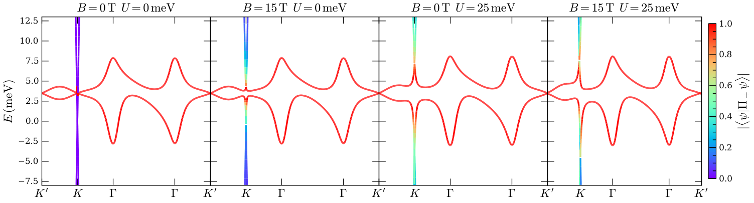
We now briefly discuss the band structure obtained from (108). For concreteness we will fix meV, and . Since we are mainly interested in the orbital effects of the field, we will ignore the Zeeman energy.
Similarly to , the main orbital effects of on the band structure are to hybridize the mirror-odd Dirac fermion with the mirror-even flat bands. Examples of the band structure in the graphene valley for various values of are shown in figure 4, where the color denotes the magnitude of the mirror-even component of the band wavefunctions.
The orbital effects of the magnetic field are rather different than in the case of TBG Kwan et al. 2020. First, when , mirror symmetry implies that the spectrum at each point is an even function of . This means that at small and small , the orbital effects on the band structure are rather weak. Secondly, despite the explicit breaking of by the magnetic field, Dirac points remain at the Moire points to an extremely good approximation for all experimentally relevant field strengths.
E.3 Effects of the field near the and points
In this section we adopt the approach used in Bistritzer and MacDonald 2011 to make some simple statements about the effects of the field on the band structure near the Moire and points, at small values of . Throughout we will focus on the graphene valley, and will neglect the physical spin degree of freedom. We will also find it convenient to follow Tarnopolsky et al. 2019 and use the notation and .
E.3.1 point
We can understand the (lack of) effects of the field at the point in a rather pedestrian manner as follows. We follow Bistritzer and MacDonald 2011 and introduce a minimal model for the modes right at by writing down the Hamiltonian
| (115) |
where we are in the basis , with the lower index denoting the layer index, the upper index denoting a reciprocal space lattice index, and where (working in units where )
| (116) |
As in the analysis of the analogous bilayer problem, there are two zero modes in this simplified 14-band problem. Let and . We will then have a zero mode provided we take
| (117) |
and that
| (118) |
with this last equation trivially satisfied as our matrices are Hermitian.
For simplicity we will now work perturbatively in . At , the zero modes have norm
| (119) | ||||
After correctly normalizing the wavefunctions, the effective Hamiltonian in the zero-mode subspace near the point then reads
| (120) | ||||
with the Fermi velocity out front confirming that when , , with the th magic angle for twisted -layer graphene Tarnopolsky et al. 2019; Bistritzer and MacDonald 2011. As expected from symmetry considerations, is independent of the magnetic field to this order.
E.3.2 point
The effects of the magnetic field near the point are slightly more interesting, due to the hybridization between the flat bands and the mirror-odd Dirac cone.
We proceed as above: near , the analogous minimal model operates in the space , where again the upper index is the layer index and the lower index is the reciprocal lattice index. Right at , the Hamiltonian is
| (121) |
There are now four zero modes. We write the first four components of each zero mode (in the above basis) as the vector ( as before). In order to have a zero mode, the components must satisfy
| (122) |
and
| (123) |
Evidently we only have zero modes if (which we already know to be the case by looking at the band structure).
To isolate the effects of the magnetic field on the Dirac cones, we will accordingly now set . Treating and as perturbations, the effective Hamiltonian in the zero mode subspace works out to be
| (124) |
When , we solve for the spectrum and find two doubly degenerate states at energies (as before, is the interlayer separation)
| (125) |
These doubly degenerate states form Dirac cones which live at the point above / below zero energy.
By computing the band structure numerically (see figure 5), one finds that when (with the first magic angle), two Dirac cones split off from the point and move along the direction normal to . To demonstrate this within the context of the present ten-band model we can consider e.g. , for which the effective Hamiltonian is
| (126) |
The determinant of this matrix vanishes at , where
| (127) |
which evidently is only a solution provided that , i.e. if , which in this approximation is the same as . Therefore when we have two Dirac cones located at the point at energies , and two at zero energy at the momenta . Since the orbital magnetic energy is much smaller than , this shift is rather small at experimentally relevant field strengths.
On the other hand, when , one finds that the two Dirac cones which split off of the point move off parallel to . To demonstrate this we may take . The Hamiltonian is then
| (128) |
Taking the determinant, one finds two doubly degenerate zero modes when , where now
| (129) |
This is only a solution if , i.e if . Note that the square root dependence of on and the linear dependence on holds on both sides of the magic angle.
References
- Cao et al. (2018a) Y. Cao, V. Fatemi, A. Demir, S. Fang, S. L. Tomarken, J. Y. Luo, J. D. Sanchez-Yamagishi, K. Watanabe, T. Taniguchi, E. Kaxiras, et al., Nature 556, 80 (2018a).
- Chen et al. (2019) G. Chen, L. Jiang, S. Wu, B. Lyu, H. Li, B. L. Chittari, K. Watanabe, T. Taniguchi, Z. Shi, J. Jung, et al., Nature Physics 15, 237 (2019).
- Sharpe et al. (2019) A. L. Sharpe, E. J. Fox, A. W. Barnard, J. Finney, K. Watanabe, T. Taniguchi, M. Kastner, and D. Goldhaber-Gordon, Science 365, 605 (2019).
- Chen et al. (2020a) G. Chen, A. L. Sharpe, E. J. Fox, Y.-H. Zhang, S. Wang, L. Jiang, B. Lyu, H. Li, K. Watanabe, T. Taniguchi, et al., Nature 579, 56 (2020a).
- Serlin et al. (2020) M. Serlin, C. Tschirhart, H. Polshyn, Y. Zhang, J. Zhu, K. Watanabe, T. Taniguchi, L. Balents, and A. Young, Science 367, 900 (2020).
- Zondiner et al. (2020) U. Zondiner, A. Rozen, D. Rodan-Legrain, Y. Cao, R. Queiroz, T. Taniguchi, K. Watanabe, Y. Oreg, F. von Oppen, A. Stern, et al., Nature 582, 203 (2020).
- Saito et al. (2020) Y. Saito, J. Ge, K. Watanabe, T. Taniguchi, E. Berg, and A. F. Young, arXiv preprint arXiv:2008.10830 (2020).
- Saito et al. (2021) Y. Saito, J. Ge, L. Rademaker, K. Watanabe, T. Taniguchi, D. A. Abanin, and A. F. Young, Nature Physics pp. 1–4 (2021).
- Wu et al. (2021) S. Wu, Z. Zhang, K. Watanabe, T. Taniguchi, and E. Y. Andrei, Nature Materials pp. 1–7 (2021).
- Chen et al. (2020b) S. Chen, M. He, Y.-H. Zhang, V. Hsieh, Z. Fei, K. Watanabe, T. Taniguchi, D. H. Cobden, X. Xu, C. R. Dean, et al., Nature Physics pp. 1–7 (2020b).
- Cao et al. (2020) Y. Cao, D. Rodan-Legrain, J. M. Park, F. N. Yuan, K. Watanabe, T. Taniguchi, R. M. Fernandes, L. Fu, and P. Jarillo-Herrero, arXiv preprint arXiv:2004.04148 (2020).
- Rozen et al. (2020) A. Rozen, J. M. Park, U. Zondiner, Y. Cao, D. Rodan-Legrain, T. Taniguchi, K. Watanabe, Y. Oreg, A. Stern, E. Berg, et al., arXiv preprint arXiv:2009.01836 (2020).
- Zhou et al. (2021) H. Zhou, T. Xie, A. Ghazaryan, T. Holder, J. R. Ehrets, E. M. Spanton, T. Taniguchi, K. Watanabe, E. Berg, M. Serbyn, et al., arXiv preprint arXiv:2104.00653 (2021).
- Balents et al. (2020) L. Balents, C. R. Dean, D. K. Efetov, and A. F. Young, Nature Physics 16, 725 (2020).
- Andrei et al. (2021) E. Y. Andrei, D. K. Efetov, P. Jarillo-Herrero, A. H. MacDonald, K. F. Mak, T. Senthil, E. Tutuc, A. Yazdani, and A. F. Young, Nature Reviews Materials pp. 1–6 (2021).
- Liu et al. (2020) X. Liu, Z. Hao, E. Khalaf, J. Y. Lee, Y. Ronen, H. Yoo, D. H. Najafabadi, K. Watanabe, T. Taniguchi, A. Vishwanath, et al., Nature 583, 221 (2020).
- Lu et al. (2019) X. Lu, P. Stepanov, W. Yang, M. Xie, M. A. Aamir, I. Das, C. Urgell, K. Watanabe, T. Taniguchi, G. Zhang, et al., Nature 574, 653 (2019).
- Yankowitz et al. (2019) M. Yankowitz, S. Chen, H. Polshyn, Y. Zhang, K. Watanabe, T. Taniguchi, D. Graf, A. F. Young, and C. R. Dean, Science 363, 1059 (2019).
- Cao et al. (2018b) Y. Cao, V. Fatemi, S. Fang, K. Watanabe, T. Taniguchi, E. Kaxiras, and P. Jarillo-Herrero, Nature 556, 43 (2018b).
- Arora et al. (2020) H. S. Arora, R. Polski, Y. Zhang, A. Thomson, Y. Choi, H. Kim, Z. Lin, I. Z. Wilson, X. Xu, J.-H. Chu, et al., Nature 583, 379 (2020).
- Khalaf et al. (2019) E. Khalaf, A. J. Kruchkov, G. Tarnopolsky, and A. Vishwanath, Physical Review B 100, 085109 (2019).
- Li et al. (2019) X. Li, F. Wu, and A. H. MacDonald, arXiv preprint arXiv:1907.12338 (2019).
- Hao et al. (2021) Z. Hao, A. Zimmerman, P. Ledwith, E. Khalaf, D. H. Najafabadi, K. Watanabe, T. Taniguchi, A. Vishwanath, and P. Kim, Science 371, 1133 (2021).
- Park et al. (2021a) J. M. Park, Y. Cao, K. Watanabe, T. Taniguchi, and P. Jarillo-Herrero, Nature pp. 1–7 (2021a).
- Cao et al. (2021) Y. Cao, J. M. Park, K. Watanabe, T. Taniguchi, and P. Jarillo-Herrero, Nature 595, 526 (2021).
- Calugaru et al. (2021) D. Calugaru, F. Xie, Z.-D. Song, B. Lian, N. Regnault, and B. A. Bernevig, arXiv preprint arXiv:2102.06201 (2021).
- Bistritzer and MacDonald (2011) R. Bistritzer and A. H. MacDonald, Proceedings of the National Academy of Sciences 108, 12233 (2011).
- Tarnopolsky et al. (2019) G. Tarnopolsky, A. J. Kruchkov, and A. Vishwanath, Physical review letters 122, 106405 (2019).
- Lei et al. (2020) C. Lei, L. Linhart, W. Qin, F. Libisch, and A. H. MacDonald, arXiv preprint arXiv:2010.05787 (2020).
- Carr et al. (2020) S. Carr, C. Li, Z. Zhu, E. Kaxiras, S. Sachdev, and A. Kruchkov, Nano letters 20, 3030 (2020).
- Vishwanath et al. (2004a) A. Vishwanath, J. E. Moore, and T. Senthil, Physical Review B 69, 054507 (2004a).
- Bultinck et al. (2020) N. Bultinck, E. Khalaf, S. Liu, S. Chatterjee, A. Vishwanath, and M. P. Zaletel, Physical Review X 10, 031034 (2020).
- Khalaf et al. (2020a) E. Khalaf, S. Chatterjee, N. Bultinck, M. P. Zaletel, and A. Vishwanath, arXiv preprint arXiv:2004.00638 (2020a).
- Chatterjee et al. (2020) S. Chatterjee, N. Bultinck, and M. P. Zaletel, Physical Review B 101, 165141 (2020).
- Khalaf et al. (2020b) E. Khalaf, P. Ledwith, and A. Vishwanath, arXiv preprint arXiv:2012.05915 (2020b).
- Lee et al. (2019) J. Y. Lee, E. Khalaf, S. Liu, X. Liu, Z. Hao, P. Kim, and A. Vishwanath, Nature communications 10, 1 (2019).
- Cornfeld et al. (2020) E. Cornfeld, M. S. Rudner, and E. Berg, arXiv preprint arXiv:2006.10073 (2020).
- Liu et al. (2021) X. Liu, K. Watanabe, T. Taniguchi, and J. Li, arXiv preprint arXiv:2108.03338 (2021).
- Ghaemi et al. (2005) P. Ghaemi, A. Vishwanath, and T. Senthil, Physical Review B 72, 024420 (2005).
- Fulde and Ferrell (1964) P. Fulde and R. A. Ferrell, Phys. Rev. 135, A550 (1964), URL https://link.aps.org/doi/10.1103/PhysRev.135.A550.
- Larkin and Ovchinnikov (1965) A. Larkin and I. Ovchinnikov, Soviet Physics-JETP 20, 762 (1965).
- Fradkin et al. (2004) E. Fradkin, D. A. Huse, R. Moessner, V. Oganesyan, and S. L. Sondhi, Physical Review B 69, 224415 (2004).
- Vishwanath et al. (2004b) A. Vishwanath, L. Balents, and T. Senthil, Physical Review B 69, 224416 (2004b).
- Po et al. (2018) H. C. Po, L. Zou, A. Vishwanath, and T. Senthil, Physical Review X 8, 031089 (2018).
- Park et al. (2021b) J. M. Park, Y. Cao, K. Watanabe, T. Taniguchi, and P. Jarillo-Herrero, Nature 592, 43 (2021b).
- Yang and Agterberg (2000) K. Yang and D. Agterberg, Physical review letters 84, 4970 (2000).
- Lin et al. (2021) J.-X. Lin, Y.-H. Zhang, E. Morissette, Z. Wang, S. Liu, D. Rhodes, K. Watanabe, T. Taniguchi, J. Hone, and J. Li, arXiv preprint arXiv:2102.06566 (2021).
- Sugiyama and Ohmi (1995) T. Sugiyama and T. Ohmi, Journal of the Physical Society of Japan 64, 2746 (1995).
- Scheurer and Samajdar (2020) M. S. Scheurer and R. Samajdar, Physical Review Research 2, 033062 (2020).
- Kawaguchi and Ueda (2012) Y. Kawaguchi and M. Ueda, Physics Reports 520, 253 (2012).
- Mukerjee et al. (2006) S. Mukerjee, C. Xu, and J. Moore, Physical review letters 97, 120406 (2006).
- Pisarski and Tsvelik (2021) R. D. Pisarski and A. M. Tsvelik, arXiv preprint arXiv:2103.15835 (2021).
- Tinkham (2004) M. Tinkham, Introduction to superconductivity (Courier Corporation, 2004).
- Buzdin et al. (2007) A. Buzdin, Y. Matsuda, and T. Shibauchi, EPL (Europhysics Letters) 80, 67004 (2007).
- Samokhin and Truong (2017) K. Samokhin and B. Truong, Physical Review B 96, 214501 (2017).
- Fischer et al. (2021) A. Fischer, Z. A. Goodwin, A. A. Mostofi, J. Lischner, D. M. Kennes, and L. Klebl, arXiv preprint arXiv:2104.10176 (2021).
- Kwan et al. (2020) Y. H. Kwan, S. Parameswaran, and S. Sondhi, Physical Review B 101, 205116 (2020).