Adaptive Channel Estimation Based on Model-Driven Deep Learning for Wideband mmWave Systems Thanks: This work was supported in part by the National Natural Science Foundation of China under Grant 61941104.
Abstract
Channel estimation in wideband millimeter-wave (mmWave) systems is very challenging due to the beam squint effect. To solve the problem, we propose a learnable iterative shrinkage thresholding algorithm-based channel estimator (LISTA-CE) based on deep learning. The proposed channel estimator can learn to transform the beam-frequency mmWave channel into the domain with sparse features through training data. The transform domain enables us to adopt a simple denoiser with few trainable parameters. We further enhance the adaptivity of the estimator by introducing hypernetwork to automatically generate learnable parameters for LISTA-CE online. Simulation results show that the proposed approach can significantly outperform the state-of-the-art deep learning-based algorithms with lower complexity and fewer parameters and adapt to new scenarios rapidly.
Index Terms:
Deep learning, hypernetwork, model-driven, channel estimation, lens antenna array, beam squintI Introduction
Beamspace multiple-input multiple-output (MIMO) implemented by a discrete lens antenna array is a promising technique for 5G wireless communications. It transforms the spatial channel into the beam domain to concentrate the signal from different directions[1], which can reduce the number of radio-frequency (RF) chains significantly and thus has been successfully employed in millimeter-wave (mmWave) communications systems. However, channel estimation is very challenging because limited measurements can be observed in the baseband.
Several channel estimation approaches have been proposed [2, 3, 4]. The support detection approach in [2] utilizes the structural characteristics of the mmWave beamspace channel to reduce the pilot overhead while maintaining reliable performance. In [3], the channel matrix is regarded as a 2D image, which converts channel estimation into image reconstruction. These approaches have been developed for narrowband mmWave systems and therefore ignore the beam squint effect in wideband mmWave systems. In [4], the successive support detection (SSD) technique based on applying successive interference cancelation can estimate the wideband channels. Its performance can be further improved if several essential characteristics of mmWave channels, such as sparsity and channel correlation between adjacent antennas and subcarriers, are considered.
Recently, deep learning (DL) has been applied to physical layer communications [5, 6, 7, 8, 9, 10], including channel state information feedback [7], signal detection[8, 9], and channel estimation [10]. As a prevailing approach, model-driven DL combines expert knowledge in wireless communications with DL and has been proved to be very effective [6, 10]. For channel estimation, a model-driven DL network unfolds the approximate message passing algorithm and can estimate narrowband beamspace mmWave channels [10]. A learned denoising-based generalized expectation consistent (LDGEC) signal recovery network is developed for wideband beamspace channel estimation [11]. These DL-based approaches can obtain better performance than traditional compressed sensing (CS)-based algorithms because of the powerful ability of DL. However, they only regard the mmWave channel as an image and use a complex denoising convolutional neural network to learn the channel structure. The inherent sparsity property of mmWave channel is not utilized, resulting in many learnable parameters and high complexity.
In this article, we investigate a model-driven DL-based channel estimator for the lens-based wideband beamspace MIMO-orthogonal frequency-division multiplexing (OFDM) system. The network structure is obtained by unfolding the iterative shrinkage thresholding algorithm (ISTA) with a few learnable parameters. Different from other DL-based channel estimator using complex image denoiser, the proposed channel estimator learns to transform the beam-frequency domain mmWave channel into the domain with sparse features, thereby enables us to adopt a simple denoiser with few trainable parameters. Leveraging a small number of key parameters in the network, we further introduce another neural network named HyperNet to generate learnable parameters online automatically. Simulation results show that the proposed approach can significantly outperform the state-of-the-art DL-based algorithms with lower complexity and fewer parameters and present fast adaptation to the channel environment.
II System Model and Problem Formulation
In this section, we first present the lens-based wideband beamspace MIMO-OFDM systems. After introducing the beam squint effect, we formulate the beamspace channel estimation as a compressed image recovery problem.
II-A mmWave Beamspace Channel Model

As illustrated in Fig. 1, we consider a lens-based wideband beamspace MIMO-OFDM system. The base station (BS) equipped with an -element lens antenna array and RF chains simultaneously serves a single-antenna user. Considering the widely used Saleh-Valenzuela channel model[4], the spatial channel at sub-carrier is given by
| (1) |
for where is the number of resolvable paths, and are the complex gain and the time delay of the -th path, respectively. Furthermore, is the array response vector and is the spatial direction at sub-carrier defined as
| (2) |
where is the frequency of sub-carrier with and representing the carrier frequency and bandwidth, respectively, is the speed of light, is the physical direction, and is the antenna spacing, which is usually designed according to the carrier frequency as . A large in wideband system causes to vary greatly in different frequency of subcarrier, and results in different spatial channel , which is called beam squint effect. When the BS is equipped with a uniform linear lens antenna array, the array response vector can be represented as
| (3) |
where represents the index of different antennas. Lens antenna array as shown in Fig. 1 can transform the spatial domain in (1) into the beamspace domain. Specifically, lens antenna array plays the role of an -element spatial discrete Fourier transform (DFT) matrix . Accordingly, the wideband beamspace channel at sub-carrier can be expressed as
| (4) |
where denotes the -th path component at sub-carrier in the beamspace domain and determined by as
| (5) | ||||
where is the Dirichlet sinc function and for are the spatial directions pre-defined by the lens antenna array.
II-B Problem Formulation
The received signal vector at the BS can be written as
| (6) |
where is the pilot transmitted at sub-carrier in instant for and , and represents a Gaussian noise vector. is the adaptive selection network that is fixed for different sub-carriers. The pilot signal is known at the receiver side and we set for convenience. The received signal in instants is given by
| (7) |
where and . In this article, low-cost -bit phase shifters are utilized in the adaptive selection network . Therefore, the elements of are randomly selected from the set with equal probability.
Because the beamspace channel vectors at different subcarriers are correlated through lens antenna array response vector , which is highly similar to a D natural image. By stacking beamspace channel vectors into a matrix and transforming the complex values into real values, we have the following signal recovery model,
| (8) |
where is the received signal in the real value domain, , and . If we regard the beam-frequency matrix as a D natural image, many compressed image recovery methods can be used here for beamspace channel estimation, which enables us to develop a model-driven DL-based channel estimation network.
III Proposed Channel Estimation Network
In this section, we propose the learnable ISTA-based channel estimator (LISTA-CE) for beamspace channel estimation. After introducing the traditional ISTA algorithm, we present the network structure.
III-A Traditional ISTA Algorithm
ISTA is a classical signal recovery algorithm in CS [12]. As we regard the beam-frequency channel as a D picture, the beamspace channel estimation problem can be regarded as the compressed image recovery problem and the ISTA algorithm can be applied to estimate the beamspace channel.
ISTA algorithm recovers the signal by updating the following steps iteratively,
| (9) |
| (10) |
where is the transformation matrix that makes the sparse in some transform domain, is the iteration index, and is the iteration stepsize. The two update steps (9) and (10) are mainly used to perform gradient descent and optimization process, respectively. Therefore, can be regarded as the noisy signal and is used to perform denoising on regularized by .
III-B LISTA-CE-based Channel Estimator

(a) Beam-frequency domain

(b) Beam-delay domain
Although ISTA is an effective algorithm to solve the compressed signal recovery problem, many numerical parameters, such as and , need to be selected manually. Furthermore, choosing a proper transformation matrix is challenging. Usually, the DFT matrix is utilized but it is not an accurate sparse transformation matrix for mmWave channel, especially for a widedband system with the beam squint effect. For example, the pseudo-color map of the beam-delay domain channel in Figure. 2(b) is obtained by taking DFT for the beam-frequency matrix in Fig. 2(a). From the figure, the beam-delay domain is not exactly sparse in the transform domain, which motivates us to utilize the DL to learn the sparse transformation matrix .

To solve the problem, we develop the LISTA-CE network. The structure of LISTA-CE is illustrated in Fig. 3, which is a revised version of ISTA algorithm by adding learnable variables. The network consists of cascade layers and each has the same structure with four modules: Module , Module , Module and Module . The input of the LISTA-CE is the received signal , and the final output is the estimation of .
In LISTA-CE, Module and Module perform channel transformation and denoising in the frequency domain while Module and Module perform channel transformation and denoising in the beam domain, respectively. Following are details on the four modules.
-
Module : can be written as
(11) which is obtained by deep unfolding the ISTA algorithm into network, and is caculated in Module , which will be introduced later. Different from (9) in the ISTA algorithm, the stepsize in (11) is learned from data and not shared for each layer. If is fixed and shared for all layers (11) is reduced to (9).
-
Module : Denote as the sparse transformation for , where and are two learnable matrices. As proven in [13], . Therefore, we can rewrite (10) as
(12) where . The optimization problem in (12) can be interpreted as the denoising problem and solved by the soft denoiser, . Furthermore, is denoted as the inverse transformation for converting the signal from the sparse transform domain to the beam-frequency domain. The network structure of is symmetric to that of , which is composed of two fully connected layers. Therefore, the closed-form solution for (12) is given by
(13) where represents the threshold of the soft denoiser in the -th layer.
-
Module : Module is similar to Module but with as input and as stepsize, that is,
(15) -
Module : To perform channel transformation and denoising in the beam domain, we need to transpose firstly because the left multiplication operation in the sparse transformation represents the transformation of the columns of the matrix. Denote the transpose operations as and the inverse operation . Therefore, can be denoted as
(16) The structures of and are similar to and , respectively, but with different weights.
From the above discussion, the learnable variables inLISTA-CE network are .
IV Adaptive LISTA-CE Network
For DL-based channel estimator, how to adapt to channel environment rapidly is significantly important. In this section, we design the LISTA-CEHyper network that introduces the HyperNet network into LISTA-CE network to adjust several trainable variables to adapt the channel environment. After introducing the network structure, we analyze the complexity of different algorithms.
IV-A LISTA-CEHyper Network

Although the LISTA-CE network has superior channel estimation performance, the training and test environment mismatch will result in performance degradation. This is because the trainable variables obtained in specific settings are not suitable for another. For example, the LISTA-CE trained with the data generated from and SNR dB will have performance degradation when tested at and SNR dB. To solve the problem, we introduce the hypernetwork [15] into the LISTA-CE. In [15], the hypernetwork can generate a small number of weights for another network based on important features. As are significantly related to the number of resolvable paths and SNR value, and are chosen as the input and output for HyperNet, respectively11 1 Noth that the number of resolvable paths can be obtained by simple channel estimator in online stage.. Denote and for convenience. Three fully connected layers are used for HyperNet, which can be written as
| (17) |
where .
We first train LISTA-CE with all possible and SNR and obtain an average model called LISTA-CEAver. Then, the learnable sparse transformations are fixed and HyperNet is introduced to generate in the online deployment phase. We denote LISTA-CE combined with HyperNet as LISTA-CEHyper as shown in Fig. 4.
| Parameters | Computational Complexity | |
| LISTA-CE | ||
| LISTA-CEHyper | ||
| LDGEC | ||
| ISTA | 2 | |
| ISTA-Net+ | ||
| SSD | 0 | |
| OMP | 0 |
IV-B Complexity Analysis
We compare the complexity of LISTA-CE with other channel estimators, including LDGEC[11], ISTA[12], ISTA-Net+[13], SSD[4] and orthogonal matching pursuit (OMP)[16]. As shown in Table I, the complexities of the SSD and the OMP algorithms are and , respectively, where is the beam windows and much smaller than ( is assumed as when ). Compared to the DL-based LDGEC network and ISTA-Net+, the proposed LISTA-CE and LISTA-CEHyper have lower computational complexity because the complexity of LISTA-CE is mainly determined by matrix multiplication, which is , while the complexity of LDGEC network is determined by matrix inversion. The computational complexity of ISTA-Net+ is , dominated by convolution operation, where is the size of the filter and and are the numbers of input and output channels of convolution, respectively, and in [13]. Although LISTA-CE has more trainable parameters than ISTA-Net+, it can achieve better performance shown by simulation results in the next section.
V Simulation Results

In this section, we provide numerical results to show the performance of the proposed adaptive model-driven DL network for wideband beamspace channel estimation. The channel matrix is generated according to the system model (1) in Section II. We assume and . The carrier frequency is GHz, the bandwidth is GHz, and the number of subcarriers is . The channel matrix is generated with , , and the maximum delay ns.

The training, validation, and testing datasets contain 10000, 1280, and 2560 samples, respectively. We set the dimensions of matrices, , , and in LISTA-CE and LISTA-CEHyper to 128, 256, and 128, respectively, and set the batch size to 64. We generate the adaptive selection network, , for each batch. The LISTA-CE is trained using the Adam optimizer with learning rate . Furthermore, the learning rate is when training the HyperNet of LISTA-CEHyper. We use the normalized mean-squared error (NMSE) as the performance metric, which is defined as
| (18) |
We firstly analyze the convergence of LISTA-CE with other channel estimation algorithms. As shown in Fig. 5, all the algorithms can converge within 10 layers except the LDGEC network. Specifically, the proposed LISTA-CE can converge within 7 layers. Therefore, the LISTA-CE network can be deployed with a small number of layers in the online stage.
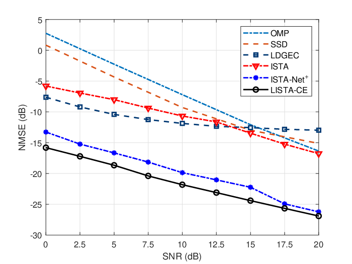
Fig. 6 compares the NMSE performance of the LISTA-CE with other channel estimation algorithms. The LISTA-CE can outperform other CS-based algorithms, including SSD, ISTA, and OMP. Compared to the LDGEC network, the LISTA-CE has better NMSE performance and lower complexity shown in section IV-B because LISTA-CE takes the sparsity of beamspace channel in the transform domain into consideration. Compared with ISTA-Net+, the LISTA-CE has approximately dB performance gain and less computational complexity shown in section IV-B. Furthermore, we utilize the DFT to transform the frequency domain into the delay domain and consider the ISTA-based channel estimator. The LISTA-CE can outperform the ISTA algorithm, as the beamspace channel in the learned sparse transform domain is much more sparse than in the delay domain.
Finally, we investigate the NMSE performance of the SSD algorithm, LISTA-CEHyper and LISTA-CEAver in Fig. 7. The LISTA-CEAver and LISTA-CEHyper are trained in and dB. After training, we test the two networks for and dB, which contains and SNR that has not been encountered in the training procedure. From the figure, LISTA-CEHyper can outperform LISTA-CEAver and the SSD algorithm in most scenarios, especially at high SNR, which indicates the LISTA-CEHyper can quickly adapt to new channel environments.
VI Conclusion
In this paper, we developed a model-driven unfolding network called LISTA-CE for wideband beamspace MIMO-OFDM channel estimation. The network can utilize the sparsity of the mmWave channel to reduce the complexity and the number of learnable variables. To adapt to the channel environment rapidly, the LISTA-CEHyper has been proposed by introducing the hypernetwork into LISTA-CE. Simulation results demonstrated that the LISTA-CE can outperform CS-based and existing DL-based channel estimation algorithms and the LISTA-CEHyper network can rapidly adapt to new environments.
Acknowledgment
This work was supported in part by the National Natural Science Foundation of China under Grant 61941104.
References
- [1] Y. Zeng, R. Zhang, and Z. N. Chen, “Electromagnetic lens-focusing antenna enabled massive MIMO: Performance improvement and cost reduction,” IEEE J. Sel. Areas Commun., vol. 32, no. 6, pp. 1194–1206, 2014.
- [2] X. Gao, L. Dai, S. Han, C. I, and X. Wang, “Reliable beamspace channel estimation for millimeter-wave massive mimo systems with lens antenna array,” IEEE Trans. Wireless Commun., vol. 16, no. 9, pp. 6010–6021, 2017.
- [3] J. Yang, C. Wen, S. Jin, and F. Gao, “Beamspace channel estimation in mmwave systems via cosparse image reconstruction technique,” IEEE Trans. Commun., vol. 66, no. 10, pp. 4767–4782, 2018.
- [4] X. Gao, L. Dai, S. Zhou, A. M. Sayeed, and L. Hanzo, “Wideband beamspace channel estimation for millimeter-Wave MIMO systems relying on lens antenna arrays,” IEEE Trans. Signal Process., vol. 67, no. 18, pp. 4809–4824, 2019.
- [5] Z. Qin, H. Ye, G. Y. Li, and B. H. F. Juang, “Deep learning in physical layer communications,” IEEE Wireless Commun., vol. 26, no. 2, pp. 93–99, 2019.
- [6] H. He, S. Jin, C. Wen, F. Gao, G. Y. Li, and Z. Xu, “Model-driven deep learning for physical layer communications,” IEEE Wireless Commun., vol. 26, no. 5, pp. 77–83, 2019.
- [7] C. K. Wen, W. T. Shih, and S. Jin, “Deep learning for massive MIMO CSI feedback,” IEEE Wireless Commun. Lett., vol. 7, no. 5, pp. 748–751, 2018.
- [8] H. Ye, G. Y. Li, and B. H. Juang, “Power of deep learning for channel estimation and signal detection in OFDM systems,” IEEE Wireless Commun. Lett., vol. 7, no. 1, pp. 114–117, 2018.
- [9] H. He, C. Wen, S. Jin, and G. Y. Li, “Model-driven deep learning for mimo detection,” IEEE Trans. Signal Process., vol. 68, pp. 1702–1715, 2020.
- [10] H. He, C. K. Wen, S. Jin, and G. Y. Li, “Deep learning-based channel estimation for beamspace mmWave massive MIMO systems,” IEEE Wireless Commun. Lett., vol. 7, no. 5, pp. 852–855, 2018.
- [11] H. He, R. Wang, S. Jin, C.-K. Wen, and G. Y. Li, “Beamspace channel estimation in terahertz communications: a model-driven unsupervised learning approach,” arXiv preprint arXiv:2006.16628, 2020.
- [12] R. Tibshirani, “Regression shrinkage and selection via the lasso,” Journal of the Royal Statistical Society. Series B (Methodological), vol. 58, no. 1, pp. 267–288, 1996. [Online]. Available: http://www.jstor.org/stable/2346178
- [13] J. Zhang and B. Ghanem, “ISTA-Net: Interpretable optimization-inspired deep network for image compressive sensing,” in IEEE/CVF Conf. Comput. Vis. Pattern Recogn., 2018, pp. 1828–1837.
- [14] K. He, X. Zhang, S. Ren, and J. Sun, “Deep residual learning for image recognition,” in IEEE/CVF Conf. Comput. Vis. Pattern Recogn., 2016, pp. 770–778.
- [15] D. Ha, A. Dai, and Q. V. Le. HyperNetworks. [Online]. Available: http://arxiv.org/abs/1609.09106
- [16] K. Venugopal, A. Alkhateeb, N. González Prelcic, and R. W. Heath, “Channel estimation for hybrid architecture-based wideband millimeter wave systems,” IEEE J. Sel. Areas Commun., vol. 35, no. 9, pp. 1996–2009, 2017.