An Energy-Based View of Graph Neural Networks
Abstract
Graph neural networks are a popular variant of neural networks that work with graph-structured data. In this work, we consider combining graph neural networks with the energy-based view of Grathwohl et al. 2019 with the aim of obtaining a more robust classifier. We successfully implement this framework by proposing a novel method to ensure generation over features as well as the adjacency matrix and evaluate our method against the standard graph convolutional network (GCN) architecture (Kipf & Welling 2016). Our approach obtains comparable discriminative performance while improving robustness, opening promising new directions for future research for energy-based graph neural networks.
1 Introduction
Graph neural networks (GNNs) are a generalization of neural networks that operate on graph-structured data, typically in the form of an adjacency matrix or graph laplacian, and feature vectors defined for the nodes. They have found success in tasks such as link prediction, node classification, and graph classification (e.g., Izadi et al. 2020, Wang et al. 2019b, Zhang et al. 2019). Alongside the empirical success, recent theoretical work has elucidated properties on their depth (Oono & Suzuki 2019), architectural alignment with algorithms (Xu et al. 2019), and their discriminative power (Xu et al. 2018). Recently, the work of Grathwohl et al. 2019 proposed viewing traditional classifiers as energy-based models, adjusting the softmax transfer function to the Boltzmann distribution, and adding an inner stochastic Langevin gradient descent (Welling & Teh 2011) loop over new samples. We extend this framework for GNNs, and introduce a novel method to ensure generation over the adjacency matrix itself along with node features. We evaluate our approach for the node classification task on the Cora, Pubmed, and Citeseer datasets and explore its generative capabilities.
2 Background and Prior Work
One of the most popular GNN architectures is the GCN architecture of Kipf & Welling 2016, which utilizes a normalized adjacency matrix with self-connections. Consider the adjacency matrix of a graph, . We define , where is the identity matrix. Let . Layer-wise propagation is given by:
| (1) |
Equation 1 follows from Kipf & Welling 2016, and multiplication by ensures symmetric normalization of the graph adjacency matrix . is the data matrix with row-wise examples, where is the number of features. is a non-linear activation function, and is a linear transformation which typically reduces the dimensionality of the data. The output of the final layer is -dimensional, where is the number of classes. This is passed through a softmax function, which is then optimized through the cross-entropy loss.
In the work of Grathwohl et al. 2019, it was noted that the softmax function can be changed in the following way: with typical machine learning classification, we are interested in a function , which maps the input data to real valued numbers, where is the number of classes, and are trainable parameters. When this is passed through a softmax function, this can be viewed as a conditional distribution of conditioned on . In viewing this as a conditional distribution, we can also see that the joint distribution is given by normalization by the partition function.
| (2) |
By marginalization of , we have the probability density function of :
| (3) |
By viewing this as a Boltzmann distribution, the energy function is given as:
| (4) |
An energy-based view of convolutional neural networks was given in the work of Xie et al. 2016, and applied to various tasks in subsequent works (Xie et al. 2017; Xie et al. 2019). Combining energy-based methods and graph neural networks has been explored in the works of Cao & Shen 2020 and Ma et al. 2019. In Ma et al. 2019, the energy is given as the sum over the node embeddings produced by a graph neural network normalized by the number of nodes, which is input into a multilayer perceptron and passed through a ReLU. In Cao & Shen 2020, an analogy to the coulomb potential is used in designing a feature pooling mechanism. Our work focuses on extending the framework of Grathwohl et al. 2019 for GNNs and the exact approach is detailed in the following section.
3 Methodology
In essence, the algorithm is a stochastic Langevin gradient descent (SLGD) loop nested inside of an stochastic gradient descent (SGD) loop. The inner SLGD loop samples the generative features over some simple distribution, and minimizes the energy of the new features using SGLD. The outer SGD loop computes the cross-entropy of the classifier, and combines the loss for the classifier as well as the generative loss, and computes the gradient. Finally, within the SGD loop, we generate new links in the adjacency matrix for nodes that are close in energy.
Batch sample and from dataset , with number of samples . Let this set be .
for all do
Replace with in , creating . Also replace with in .
for do
end for
Let (energy of the graph with the original features);
;
Add to .
The key factor for convergence when using stochastic Langevin gradient descent training with graph structured data is the renormalization by the total graph energy. The intuitive justification is that the gradient correction for the features of a node takes into account the total energy of the graph, since the messages are passed over the entire graph in the forward pass. The generative loss, , ensures that the energy of the original classifier over the selected indices is close to the energy of the generative features. This encourages their probabilities to be close to each other.
In addition to the generation over features, we have incorporated generation over the adjacency matrix itself. The motivation for this stems from the fact that for traditional machine learning models, samples are thought to be independent but that need not be the case for graph structured data as nodes are connected by edges. We use the energy of a sample as a quantitative measure to incorporate edges between the sampled data and existing graph. We compare the energy of two nodes, and add a link to the graph if the difference between the energy of two nodes is within the threshold . For stability, we do this once every 50 epochs. In the complex networks literature (e.g., Krioukov et al. 2010), which has connections to the statistical mechanics literature, the connection probability of two nodes can be given by the Fermi-Dirac distribution. Under this assumption, two nodes that are close in energy have a high probability of being connected.
4 Experimental results
To evaluate our approach for training an energy-based GNN, three citation network datasets are considered – Cora, Pubmed and Citeseer. In Table , the reported accuracies are the average performance on the test set for 5 runs with random initialization, with a train-test split following that of Kipf & Welling 2016. The deep graph library (DGL) framework (Wang et al. 2019a) is utilized for implementing the GCN upon which the energy based framework was implemented. The hyperparameters used in the experiments are given in Table 1. GCN-JEMO corresponds to the model with an additional term in the loss function which encourages the weight matrix for each layer to be orthogonal. We observe better performance with this additional constraint that promotes weight orthogonality:
| (5) |
where denotes the standard Frobenius norm .
| Model | CORA | Pubmed | Citeseer |
|---|---|---|---|
| GCN | 81.5 | 79.0 | 70.3 |
| GCN-JEM (ours) | 82.44 | 77.04 | 67.28 |
| GCN-JEMO (ours) | 83.66 | 77.6 | 66.72 |
It should be noted that some papers for the Cora and PubMed datasets appear to use different training/test splits than the one used in the original GCN paper. To be consistent with the literature, we use the original train/test splits in the GCN paper (Kipf & Welling 2016).
Our technique is in a sense architecture agnostic and can be used with any graph neural network with a similar message-passing scheme. In our study, we use the vanilla GCN (Kipf & Welling 2016) as a baseline comparison. In theory, we could adapt our technique with any of the leading architectures.
| Parameter | Value |
|---|---|
| epoch | 500 |
| learning rate | 0.01 |
| SGLD lr | 1 |
| SGLD steps | 20 |
| 0.05 | |
| SGLD noise | 0.01 |
| Sampling batch size | 32 |
5 Discussion
Our experimental results do not consistently improve the accuracy across the three datasets (an improvement for CORA is obtained), but it should be noted that the main focus of Grathwohl et al. 2019 was to improve the robustness of classifiers while having discriminative performance comparable to other top performing models. In Grathwohl et al. 2019, the authors compare their method to other hybrid models, and in fact lose accuracy compared to a purely discriminative model. As such, the generative capabilities of the proposed model is explored.


Spectrum of the adjacency matrix: In Figure 1, the spectrum of the original adjacency matrix and the spectrum of the generative adjacency matrix for the Cora dataset is shown. The -axis is the eigenvalue, and the -axis is the count of the eigenvalue with log scaling. The number of bins is set at . It is seen that the spectrum of the generative adjacency matrix resembles that of the spectrum of the original adjacency matrix. By only adding links to nodes that are close in energy, it is thought that the generative is only adding short cycles. The number of closed paths of length can be computed with the following formula:
| (6) |
Where is the spectrum of the adjacency matrix. The cycles of length are computed at for the original matrix, and for the generative matrix.
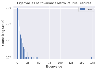
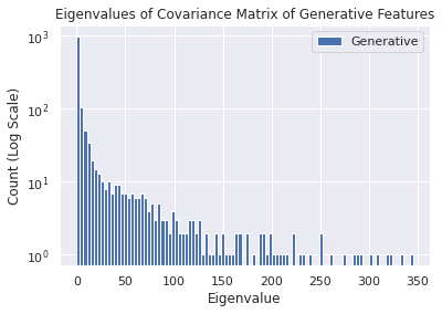
Spectrum of the feature covariance matrix: In Figure 2, the spectrum of the covariance of the original features as well as the covariance of the generative features for the Cora dataset are shown. The -axis is the eigenvalue, and the -axis is the count with log scaling. The number of bins is set at . The generative features add high covariance eigenvalues, which may add robustness against adversarial examples. It is hypothesized that if the features have more variance, then the classifier is less likely to be overtuned to the dataset.


Confidence in predictions: In Figure 3, the confidence of the prediction over the training dataset is shown for both the discriminative and generative models, where confidence is the max of the softmax of the output. The -axis is the confidence in the prediction, and the -axis is the count at regular scaling. The number of bins is set to . It is seen that the generative model overall is less confident in its predictions.
One metric to measure the calibration of a classifier is the Expected Calibration Error (ECE). First, one computes the confidence in the predictions of the dataset. Then, one bins these into equally spaced buckets. The ECE measures the absolute difference between the average accuracy over that bucket and the average confidence, weighed by the cardinality of the bucket over the total number of samples. For a perfectly calibrated classifier, this value will be 0 for any choice of , the number of buckets.
| (7) |
We compute an ECE of for the generative model and for the discriminative model over the test set of Cora (lower is better).
5.1 Future directions
Combining the energy-based framework with graph neural networks presents promising new directions for further research, both from a graph generation and theoretical point-of-view. One point of further exploration is exploring the limitations of depth as set out in Oono & Suzuki 2019. The paper posits that GNNs are limited in depth due to the action of repeated application of the graph operator. It is thought that this can be ameliorated by perturbing at every layer within the generative framework proposed in this work. Another direction for future work would be in utilizing our generative model for tasks in computational chemistry and bioinformatics tasks, where graph structure is abound, and where many tasks are inverse problems–given some chemical property that one requires, what is the structure that gives that property? Such tasks are thought to be apt for a generative graph model.
References
- Cao & Shen (2020) Yue Cao and Yang Shen. Energy-based graph convolutional networks for scoring protein docking models. Proteins: Structure, Function, and Bioinformatics, 88(8):1091–1099, 2020.
- Grathwohl et al. (2019) Will Grathwohl, Kuan-Chieh Wang, Jörn-Henrik Jacobsen, David Duvenaud, Mohammad Norouzi, and Kevin Swersky. Your classifier is secretly an energy based model and you should treat it like one. arXiv preprint arXiv:1912.03263, 2019.
- Izadi et al. (2020) Mohammad Rasool Izadi, Yihao Fang, Robert Stevenson, and Lizhen Lin. Optimization of graph neural networks with natural gradient descent. arXiv preprint arXiv:2008.09624, 2020.
- Kipf & Welling (2016) Thomas N Kipf and Max Welling. Semi-supervised classification with graph convolutional networks. arXiv preprint arXiv:1609.02907, 2016.
- Krioukov et al. (2010) Dmitri Krioukov, Fragkiskos Papadopoulos, Maksim Kitsak, Amin Vahdat, and Marián Boguná. Hyperbolic geometry of complex networks. Physical Review E, 82(3):036106, 2010.
- Ma et al. (2019) Tengfei Ma, Junyuan Shang, Cao Xiao, and Jimeng Sun. Genn: predicting correlated drug-drug interactions with graph energy neural networks. arXiv preprint arXiv:1910.02107, 2019.
- Oono & Suzuki (2019) Kenta Oono and Taiji Suzuki. Graph neural networks exponentially lose expressive power for node classification. arXiv preprint cs.LG/1905.10947, 2019.
- Wang et al. (2019a) Minjie Wang, Lingfan Yu, Da Zheng, Quan Gan, Yu Gai, Zihao Ye, Mufei Li, Jinjing Zhou, Qi Huang, Chao Ma, Ziyue Huang, Qipeng Guo, Hao Zhang, Haibin Lin, Junbo Zhao, Jinyang Li, Alexander J Smola, and Zheng Zhang. Deep graph library: Towards efficient and scalable deep learning on graphs. ICLR Workshop on Representation Learning on Graphs and Manifolds, 2019a. URL https://arxiv.org/abs/1909.01315.
- Wang et al. (2019b) Rui Wang, Bicheng Li, Shengwei Hu, Wenqian Du, and Min Zhang. Knowledge graph embedding via graph attenuated attention networks. IEEE Access, 8:5212–5224, 2019b.
- Welling & Teh (2011) Max Welling and Yee W Teh. Bayesian learning via stochastic gradient langevin dynamics. In Proceedings of the 28th international conference on machine learning (ICML-11), pp. 681–688. Citeseer, 2011.
- Xie et al. (2016) Jianwen Xie, Yang Lu, Song-Chun Zhu, and Yingnian Wu. A theory of generative convnet. In International Conference on Machine Learning, pp. 2635–2644. PMLR, 2016.
- Xie et al. (2017) Jianwen Xie, Song-Chun Zhu, and Ying Nian Wu. Synthesizing dynamic patterns by spatial-temporal generative convnet. In Proceedings of the ieee conference on computer vision and pattern recognition, pp. 7093–7101, 2017.
- Xie et al. (2019) Jianwen Xie, Song-Chun Zhu, and Ying Nian Wu. Learning energy-based spatial-temporal generative convnets for dynamic patterns. IEEE transactions on pattern analysis and machine intelligence, 2019.
- Xu et al. (2018) Keyulu Xu, Weihua Hu, Jure Leskovec, and Stefanie Jegelka. How powerful are graph neural networks? arXiv preprint arXiv:1810.00826, 2018.
- Xu et al. (2019) Keyulu Xu, Jingling Li, Mozhi Zhang, Simon S Du, Ken-ichi Kawarabayashi, and Stefanie Jegelka. What can neural networks reason about? arXiv preprint arXiv:1905.13211, 2019.
- Zhang et al. (2019) Zhen Zhang, Jiajun Bu, Martin Ester, Jianfeng Zhang, Chengwei Yao, Zhi Yu, and Can Wang. Hierarchical graph pooling with structure learning. arXiv preprint arXiv:1911.05954, 2019.