Observation of non-Abelian topological semimetals and their phase transitions
Abstract
Topological phases of matter lie at the heart of physics, connecting elegant mathematical principles to real materials that are believed to shape future electronic and quantum computing technologies. To date, studies in this discipline have almost exclusively been restricted to single-gap band topology because of the Fermi-Dirac filling effect. Here, we theoretically analyze and experimentally confirm a novel class of multi-gap topological phases, which we will refer to as non-Abelian topological semimetals, on kagome geometries. These unprecedented forms of matter depend on the notion of Euler class and frame charges which arise due to non-Abelian charge conversion processes when band nodes of different gaps are braided along each other in momentum space. We identify such exotic phenomena in acoustic metamaterials and uncover a rich topological phase diagram induced by the creation, braiding and recombination of band nodes. Using pump-probe measurements, we verify the non-Abelian charge conversion processes where topological charges of nodes are transferred from one gap to another. Moreover, in such processes, we discover symmetry-enforced intermediate phases featuring triply-degenerate band nodes with unique dispersions that are directly linked to the multi-gap topological invariants. Furthermore, we confirm that edge states can faithfully characterize the multi-gap topological phase diagram. Our study unveils a new regime of topological phases where multi-gap topology and non-Abelian charges of band nodes play a crucial role in understanding semimetals with inter-connected multiple bands.
With the advent of topological phases, the past few years have seen rapid progresses in classifying topological states of matter. Upon analyzing the manner in which bands transform at high-symmetry momenta, one can deduce compatibility relations Kruthoff et al. 2017 conveying how many different classes of gapped band structures exist on a lattice geometry with a given set of symmetries (see Fig. 1A for schematic illustration). Moreover, by comparing to real space, efficient schemes were proposed that can discern which of these classes can be deemed topological by absence of an atomic limit Po et al. 2017; Bradlyn et al. 2017.
Here, we consider an exotic type of topological phases beyond the above paradigms that, instead, depend on topological charge conversion processes when band nodes are braided with respect to each other in momentum space or recombined over the Brillouin zone. The braiding of band nodes is in some sense the reciprocal space analog of the non-Abelian braiding of particles in real space and is manifested by a new topological invariant, the Euler class, Wu et al. 2019; Ahn et al. 2019; Bouhon et al. 2020a. Considering a kagome model and its realization in acoustic metamaterials, we uncover a rich interplay between these concepts and crystalline symmetries Fu 2011; Slager et al. 2012; Bouhon and Black-Schaffer 2017; Fang et al. 2012; Slager 2019; Cornfeld and Carmeli 2021 and further experimentally confirm the above physics in acoustic metamaterials by tuning their geometry. The rich phase diagram features unavoidable intermediate phases featuring band degeneracies at high symmetry point with unconventional dispersion features that have a topological origin that is not captured by representation theory alone Yang and Nagaosa 2014; Bradlyn et al. 2016. In addition, we reveal the edge physics associated with the non-Abelian band braiding within the above context.

[h]
Euler class and multi-gap topology
While the study of topological materials and their interplay has resulted in a thriving field on both the theoretical and experimental front, Euler class provides a new paradigm of topological phases. Akin to Chern numbers, systems that feature combined twofold rotation and time reversal symmetry, , or combined parity and time reversal symmetry, , can be described by a real Hamiltonian that can exhibit this topological invariant Wu et al. 2019; Ahn et al. 2019; Bouhon et al. 2020a. From a more physical perspective, these new forms of topology can be best understood as being the consequence of a perspective that takes into account multiple band gap conditions Bouhon et al. 2020b.
For instance, one can revert to a minimal Euler model that arises in a three-band system featuring two gapless bands and a gapped band, as detailed in Fig. 1. The Euler invariant manifests itself by the presence of a number of irremovable band nodes between the two gapless bands. Conventionally, semi-metals host nodes with opposite topological charges that can be pairwise annihilated as the consequence of the celebrated Nielsen-Ninomiya theorem. In the Euler case, however, the nodes have an additional frame charge that is the same for the irremovable nodes. The according inability to annihilate the band nodes reveals the topological obstruction that the topological Euler number imposes.
The above counter-intuitive possibility is intimately tied to both the real-valued form of the Hamiltonian and the concept of orientability. Namely, the reality condition ensures that the set of Eigenstates can be interpreted as an oriented orthonormal frame, or dreibein when restricting to three-band systems as in this work. Decomposing the 3D rotation matrix along paths encircling stable nodes we can then directly compute the acquired angle of the monopole, or frame charge, reflecting the geometry of SO(3) rotations Johansson and Sjöqvist 2004; Bouhon et al. 2020a. Then, as a component of the spectral decomposition of the Hamiltonian, this frame is only defined up to a sign for each Eigenstate. Hence, the frame charges of the nodes are related to the flag variety Wu et al. 2019; Bouhon et al. 2020a. As a consequence, the band nodes correspond to -disclinations in a biaxial nematic liquid crystals Alexander et al. 2012; Liu et al. 2016; Volovik and Mineev 2018 and the charges associated to nodal points within three bands take values in the conjugacy classes of the quaternion group, i.e. with . Specifically, in our case and characterize single nodes in each of the respective gaps, represents a pair of nodes in each gap, and () captures the stability of two nodes of the same gap Wu et al. 2019; Tiwari and Bzdušek 2020.
Using the fact that frame charges behave as quaternions, we then directly uncover a geometric relation between the braiding process involving the two gaps Wu et al. 2019; Ahn et al. 2019; Bouhon et al. 2020a, as explained in Fig. 1B, and the Euler invariant. Specifically, one can start from a trivially gapped system and create pairs of band nodes in the two gaps having charges and , respectively. Each gap hosts a pair of oppositely-valued band node charges, which may be gapped out in a reverse process to arrive back at the trivial system (i.e., Euler class ). However, braiding a node residing in the first band gap, say , along a node in the second gap, say , produces in each gap a pair of nodes that cannot be annihilated upon collision (non-zero Euler class), which can effectively be phrased in terms of the conversion of the non-Abelian charges of the braided nodes rendering, e.g., the combination Wu et al. 2019; Ahn et al. 2019; Bouhon et al. 2020a, see Fig. 1. We note that an additional trivial band can thus trivialize the Euler model by the reverse braid process, showing that this enigmatic topology is formally a form a fragile topology, albeit rather distinct from the symmetry eigenvalue indicated variant Po et al. 2018; Bouhon et al. 2019; Song et al. 2019; Peri et al. 2020; Song et al. 2020.
In the above we have implicitly applied the concept of patch Euler class, defined for a patch in the Brillouin zone that contains the nodes of pairs of bands isolated from all other bands by an energy gap Bouhon et al. 2020a. The patch Euler class is thus computed independently of the potential presence of nodes connecting the two bands under consideration with other bands outside the patch.
Dirac Strings
The concrete setup that we will present shortly, however, takes the above insight to a next level and features a profound role of so-called Dirac strings in one band gap that affect the charges in the other. Dirac strings naturally appear when considering smooth representations of real eigenvectors, marking the necessary discontinuity of the gauge sign upon the creation of any pair of nodes Ahn et al. 2019. They are the 2D analogue within the real context of the Dirac strings of 3D Weyl semimetals within the complex context. It can be shown that by specifying a relative sign as the charge of each node within a gap (which we represent below through open/filled symbols for opposite charges and with distinct symbols for different gaps, e.g., , and , for the first and second gap respectively) as well as the Dirac strings connecting such nodes, we obtain a picture that exhaustively captures the topological content of the band structure.
To this end only a few rules have to be taken into account in order to predict the outcomes of the braiding of nodes. Namely, () each DS must connect one pair of same-gap-nodes, i.e. , , , etc., () the charge of a node switches when crossing the DS of a neighboring (adjacent) gap, i.e. , , () any couple of Dirac strings in the same gap can be recombined through the permutation of the end nodes, i.e. . We note that these rules are merely different representations of a consistent charge assignment, and refer to Supplementary Note A for a detailed account on deforming DS configurations.
Interplay with kagome geometry
The above view relating Euler forms and multi-gap topologies can be made rigorous using homotopy theory Bouhon et al. 2020b, culminating in more intricate insulating Euler class topologies. However, it is all we need to put the physics presented here into perspective. Starting from a kagome geometry, we combine a symmetry-eigenvalue analysis together with the above new topological concepts to unravel topological transitions between a rich variety of phases arising via a symmetry-constrained braiding of band nodes. These insights are then accompanied by direct signatures that reveal Euler class physics Ünal et al. 2020.
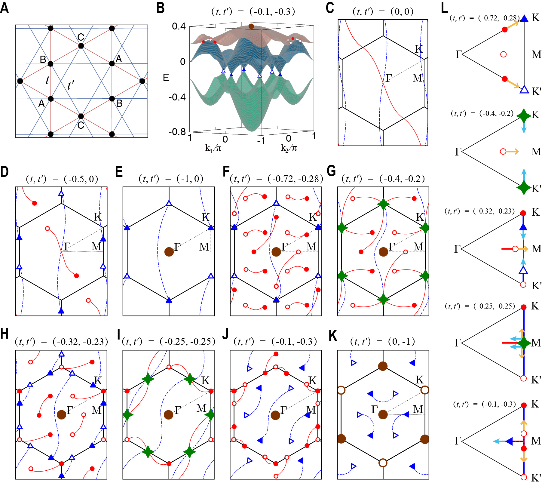
We now turn to the specific model that will be the center stage to put the above ideas into play. We depart from -orbitals located at (see Fig. 2A) and include the NN and the NNN couplings to arrive at the following Hamiltonian,
| (1) |
written in the Bloch basis using the Zak gauge (see Supplementary Note B), with
| (2) |
The wavevector is given over the Brillouin zone in units of the reciprocal lattice vectors, i.e., with where are the reciprocal primitive vectors dual to , and () are the NN (NNN) couplings. In the following, we refer to the point as , the and points, and the , and points.
Topological phase diagram
We start from the simplest gapped phase and then introduce band nodes, to study the evolution and braiding of the nodes along a designed trajectory in parameter space. To this end, consider the gapped atomic insulating phase that breaks symmetry, by setting and . This system then has the band energies , , and , and the corresponding Bloch eigenstates , , and . In the following, we refer to gap I as the (partial) energy gap between bands 1 and 2, and gap II as the (partial) energy gap between bands 2 and 3.
The Berry phase factors for each band () over a non-contractible path where is a reciprocal lattice vector, i.e., with the -th band projector , are then readily given by
| (3) |
where we have used the periodic gauge for the Wilson loop integration Bouhon and Black-Schaffer 2017. Berry phases on non-contractible path are also referred as Zak phases Zak 1989. Taking and writing the vector , we find (modulo )
| (4) |
While the total band bundle of the three bands is orientable, i.e., the above Berry phases sum to in each direction, the ‘flag bundle’ (where we consider each band separately) is non-orientable as indicated by the non-zero Berry phases Bouhon et al. 2020b. Each -Berry phase indicates the presence of an odd-number of Dirac strings crossing perpendicularly the path of integration Ahn et al. 2018. The corresponding configuration of Dirac strings of this non-orientable atomic phase is shown in Fig. 2C where the Dirac string across gap I (DSI) is shown as a blue dashed line, and the Dirac string across gap II (DSII) as a red full line. It is remarkable that, as long as is preserved, the system cannot exhibit a fully trivial and orientable band structure, as will become clear below.
We now deform the model to obtain the simplest kagome model while restoring the symmetry. This is done by setting and . During the deformation there is a band inversion in each gap, thus creating two simple nodes of opposite charges in each gap, see Fig. 2D where and . The final configuration shown in Fig. 2E has two simple nodal points at the K and points in gap I (small blue triangles) that are connected by DSI (a Dirac string in gap I), and a double nodal point at in gap II (large brown circle). DSII is fully resorbed, and DSI has been chosen as to avoid the nodes of gap II. While these degeneracies, at s and , correspond to the two-dimensional irreducible representations and of the elementary band representation of -atomic orbitals at Wyckoff position of layer group L80 ITC 2006; ITC 2010, our analysis reveals the origin of stability of the double node at which is independent of the crystalline symmetries. Indeed, in order to go from Fig. 2D to Fig. 2E, DSI must cross one node of gap II and flip its charge (cf. rule () above, and the left column of Fig. S-3 in Supplementary Note A). As a consequence, the two nodes in gap II in the vicinity of have equal charge leading to a patch Euler class of (equivalently, a frame charge of ), thus indicating that they cannot be annihilated. A robust associated feature of the nontrivial patch Euler class of the stable double node degeneracy (at ), is its quadratic dispersion in all directions, as opposed to the linear dispersion (“Dirac cone”) around the double degeneracy (at ), see Fig. 1C. We emphasize that the pair of nodes at are stable upon the breaking of point group of the kagome lattice (L80) as long as the symmetry is preserved as predicted by the Euler class (frame charge) obstruction.
Symmetry-constrained braiding of band nodes
We come to a main feature that concerns the transfer of the double degeneracies from one gap to the other. We focus here on the point and discuss the analog for the point in the Supplementary Note C (see Fig.S-5). These processes thrive on the Kagome symmetries that necessitate triple degeneracies at , (see below), and in the charge conversion processes. Namely, we show that the braiding of nodes effectively acts as a pump of simple nodes (at ) and double nodes (at ) from one gap to the other other, mediated by triply-degenerate points.
The process is illustrated through Figs. 2E-K, while the irreducible representation (IRREP) content of the band structures is detailed in Fig. S-4 of Supplementary Note C. First, two sextets of nodes in gap II (red circles) are generated from , i.e., there are two nodes on each of the three -- and -- lines (Fig. 2F). These extra nodes must appear together upon a band inversion at as a result of the crystalline symmetries () of the system, see Figs. S-4a-b that show the reordering of IRREPs and the resulting symmetry protected nodes inside the Brillouin zone. Importantly, the charge configuration precisely captures the fact that the nodes can be annihilated in the reversed process. In particular, the Euler class (frame charge) of the nodes at is preserved. Then, the ---nodes reach the points first, thus realizing two triply-degenerate points (represented by the green stars in Fig. 2G) which is the necessary step upon a band inversion at () (see Figs. S-4a-c). Each triply-degenerate point then gives birth to one simple node in gap II at the () point, and three simple nodes in gap I (blue triangles) on the -M- lines (Fig. 2H). This follows by symmetry from the band inversion at () (see Fig. S-4d). We note that the step from Fig. 2G to H requires the recombination of Dirac strings (cf. rule ). Also, defining a loop around the () encircling the ---nodes in Fig. 2F, the frame charge of is conserved through Fig. 2G and Fig. 2H. Then, the ---nodes in gap II and the ---nodes in gap I join at the points, realizing three triply-degenerate points (Fig. 2I). Contrary to the previous case, these triple points are not imposed by symmetry (Figs. S-4d-e) but are rather model specific (see below). Each triply-degenerate point then gives birth to two ---nodes in gap I and two ---nodes in gap II (Fig. 2J). This results by symmetry from the band inversion at (Figs. S-4f). Also, the transition of charges through Fig. 2H-I-J requires the flip of the charges of the nodes in gap II after crossing the DSI (rule ()). The full band structure at this step of the process (Fig.2J) is shown in Fig. 2B. The ---nodes in gap II then reach the and points, where two double nodes are formed, each with a nontrivial patch Euler class (frame charge ) (Fig. 2K). We note that the step Fig. 2J-K requires the recombination of DSI (rule ()).
Key bulk features
Given the complexity of the conversion processes, we recapitulate some of the essential features lying at the core of the symmetry-constrained braiding for which symmetry and topology must be married in a new way. In our framework, we already mentioned the quadratic dispersion in all directions of the double nodes, e.g. at (Fig. S-4a) and at (Fig. S-4g). This is a robust feature of the non-trivial patch Euler class (frame charge ) of two stable nodes (see Fig. 1C) that sit on top of each-other as a result of a crystalline symmetry (i.e. at , and at ) Lenggenhager et al. 2020.
It is known that three-dimensional semimetals with symmetry and fourfold or sixfold rotational symmetry can host a double degeneracy at that gives rise to a triply degenerate node along the -rotation axis Zhu et al. 2016; Kim et al. 2018; Lenggenhager et al. 2020. This is also another important aspect of the bulk topology here for the (and , see SM C) point, that are unavoidable by symmetry upon the pumping of nodes from one gap to the other. On the contrary, the triply-degenerate point at the , and points only exist as long as -dependent same-sub-lattice-site hopping terms are discarded (i.e., , ). In other words, by discarding intra-sublattice-site hoppings the kagome model cannot be gapped, i.e., the three bands must remain connected through simple, double, and triple nodes.
Very interestingly, the frame charge associated to one triply-degenerate node reflects again the dispersion of the bands. A frame charge of implies a triple node with two linear bands (at in Fig. S-4c), while a frame charge of implies a parabolically-dispersed triply-degenerate point (at in Fig. S-5b), as shown in Fig. 1C.
Edge projections
The above determination of bulk charges (i.e., non-Abelian frame charges, Dirac strings, and patch Euler class) also allows us to systematically obtain the Zak phases for different edge projections and predict the existence of edge branches in the different gaps. Indeed, whenever the Zak phase’s integration path crosses an odd (even) number of Dirac strings, we get a -(-)Zak phase. Zak has shown that in one-dimensional quantum systems (here the 1D slices of the 2D phase) the Zak phase, obtained from the projection to a group of bands isolated by an energy gap, predicts the location of the center of charge of the Bloch eigenstates (i.e. the expectation value of the position operator) Zak 1989. The bulk-edge correspondence linking the value of the Zak phase with the presence of an edge state follows from the conservation of charges and the incommensurability between the number of atomic orbitals, located at the sites that compose the finite 1D system, and the number of band-projected orbitals originating from the different gap-separated blocks of bands. Incommensurability, also often called charge anomaly Su et al. 1979, typically happens when there is a mismatch between the locations of the atomic and the band orbitals.
We consider the zigzag (see below) and armchair (in Supplementary Note G) edges, which are defined with respect to the honeycomb structure underlying the kagome lattice (i.e. connecting the centers of every small triangle forming the kagome lattice), see the green lines in Fig. 3C and F. The integration path in momentum space for a given edge geometry is dictated by the redefinition of the Brillouin zone within the coordinates dual to the edge axes , where is perpendicular to the edge and remains a good quantum number thanks to the translational invariance along the edge. Then, is the integration axis for the Zak phase. The edge-oriented Brillouin zones are given as the insets of Fig. 5 for the zigzag edges, and of Fig. S-11 for the armchair edges, where is the vertical axis in both cases. Crucially, we find that there is an edge state, given an edge projection and an energy gap, whenever the Zak phase is zero. This matches with the fact that the atomic orbitals are located on the boundary of the unit cell (i.e. Wyckoff position ). In other words, for the given geometry, the -Zak phase indicates a charge anomaly and hence the existence of a topological edge state.
From the known bulk charge configuration, we then expect observable conversions of the edge states through the braiding process. Inversely, the conversion of the edge states through the different steps of the phase diagram provides an indirect manifestation of the bulk braiding of nodes. We note in this regard recent work on one-dimensional gapped real three-band Hamiltonian realized in electric circuits Guo et al. 2020, where the relation between Zak phases and non-Abelian charges has been observed. Within this work we consider genuine Euler class semimetallic materials, a topological phase that has no one-dimensional equivalent, and the according braiding process (which similarly requires two spatial dimensions) leading to these phases. Moreover, the discussed unavoidable bulk features, such as stability of nodes, the pumping effect and triple degeneracies upon braiding of nodes, are universal and applicable outside the tunable realm of metamaterials. Indeed, we emphasize that, while relations between Zak phases and edge states are well-defined, a general bulk-boundary correspondence in terms of the non-Abelian frame charges is yet to be formally understood.
Acoustic metamaterials
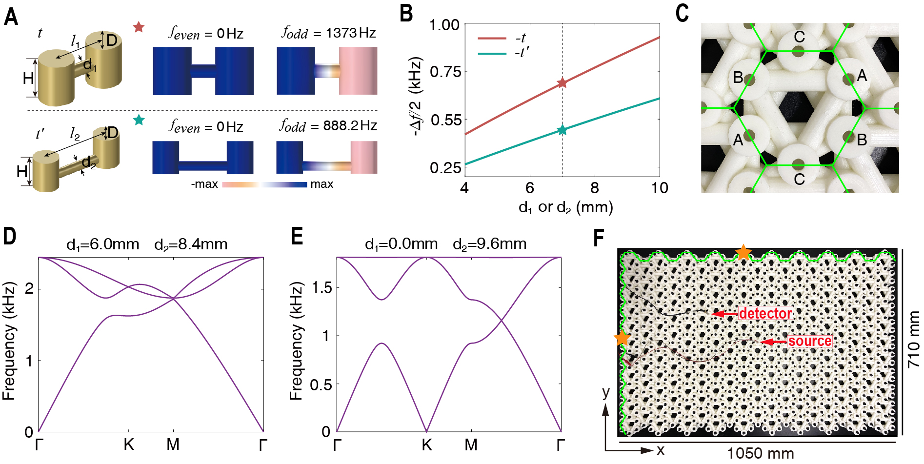
To verify the above evolution and braiding of the band nodes, we created a physical realization of the kagome model using acoustic metametarials based on coupled acoustic resonators. Such acoustic metamaterials have been demonstrated as a highly-tunable and versatile platform for the study of topological phenomena Yang et al. 2015; Xiao et al. 2015; He et al. 2016; Lu et al. 2017; Li et al. 2017; He et al. 2018; Xue et al. 2019; Ni et al. 2019; Zhang et al. 2019. In our design, each acoustic resonator is a hollow cylinder with an air region of height and diameter encapsulated by a shell made of resin which confines the acoustic waves. These acoustic resonators play the roles of the sites in the kagome model. The nearest-neighbor (NN) and next-nearest-neighbor (NNN) couplings between the acoustic resonators are then achieved through the air tubes connecting the resonators with diameters and , respectively. The acoustic metamaterial, with a lattice constant of mm, is fabricated using the 3D printing technology based on photosensitive resin (see more details in Supplementary Note D. As illustrated in Fig. 3A, two acoustic resonators connected with a tube support two hybridized modes (even and odd modes) with a splitting . The coupling between the two resonators is equal to . We find that for both the NN and NNN couplings, their strength can be tuned at will through the diameters and (Fig. 3B). A photo of the unit-cell of the fabricated acoustic metamaterial is shown in Fig. 3C for mm and mm. The corresponding acoustic band structure is presented in Fig. 3D, showing the anticipated triple degeneracy at the M point (similar to the case in Fig. 2I). By tuning the diameters to and mm, the acoustic band structure with quadratic band touching at the and M points is realized (see Fig. 3E; similar to the case in Fig. 2K). Although the acoustic setup does not exactly match the tight-binding model, the acoustic metamaterial effectively reproduces all topological band features of the model, as shown below.
Characterization of the bulk bands
The experimental set-up for the measurement of the acoustic band structures is shown in Fig. 3F. The fabricated acoustic metamaterial has 200 unit-cells, making a rectangular geometry of mmmm. The upper and left edge boundaries are closed (except at the corners) while the lower and right edge boundaries are open. Such a structure is optimized for the measurements of the bulk and edge bands (see Supplementary Note E). For the measurement of the bulk bands, an acoustic source is placed into a resonator at the center of the sample to excite the bulk Bloch waves at various frequencies from 5Hz to 3kHz. A probe microphone scans the acoustic pressure at all other resonators. By Fourier-transforming the detected acoustic pressure distributions at each excitation frequency, we obtain the acoustic bulk band structure for each of the six fabricated acoustic metamaterials (see Supplementary Note F for details). Similarly, when measuring the edge bands, the acoustic source is placed at the center of the armchair or zigzag edge boundary (labeled by the yellow stars), while the acoustic pressure distributions along the edge boundaries are scanned at various excitation frequencies.
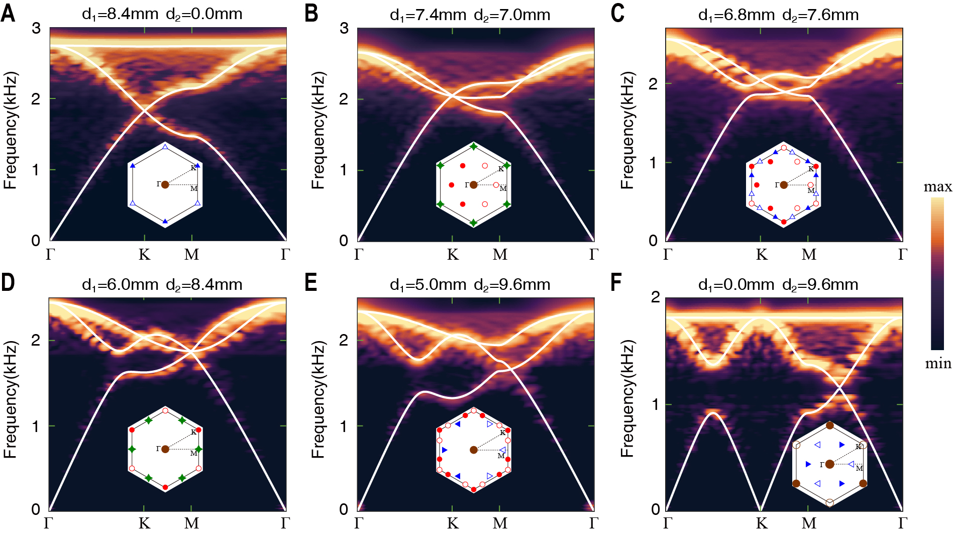
We first measure the bulk bands for the six acoustic metamaterials, similar (but not exactly identical) to the cases in Figs. 2E, 2G-2K along the braiding trajectory. As presented in Fig. 4, the measured acoustic band structures agree excellently with the calculated acoustic band structures. These band structures faithfully regenerate the band nodes evolution in Fig. 2. Specifically, in Fig. 4A ( mm and ), the acoustic metamaterial exhibits the usual dispersion of the kagome lattice with two Dirac nodes at the K and K′ points in gap I as well as a quadratic band touching at the point in gap II. Another known feature of the familiar kagome lattice is that the third band emerges as a flat band. In Fig. 4B, by tuning the diameters of the connecting tubes to mm and mm, the triple degeneracy emerges at the K and K′ points. Meanwhile, the Dirac nodes are transferred to gap II in the K--K′ lines. In Fig. 4C ( mm and mm), the triple degenerate points split into three Dirac nodes: one at the K (or K′) point in gap II and two on the K-M-K′ lines in gap I. In Fig. 4D, by tuning the parameters to mm and , the Dirac nodes in the K--K′ lines in gap II and those in the K-M-K′ lines in gap I coalesce to form the triple degeneracy at the three M points. Meanwhile, the Dirac nodes in gap II remains at the K and K′ points. In Fig. 4E ( mm and mm), the triple degeneracy splits into Dirac nodes again. But now, the Dirac nodes lying on the K--K′ lines are transferred into gap I, while the Dirac nodes on the K-M-K′ lines are transferred into gap II. The latter Dirac nodes eventually coalesce at the K and K′ points to form quadratic band touching, as shown in Fig. 4F by setting mm and mm. Several remarks are in place: First, the whole process indicates that the degeneracy at the K point in gap I switches with the degeneracy on the - and - lines in gap II. By changing the charges of the nodes in gap II, the reciprocal braiding processes lead to a double node at the () point in gap II with nontrivial patch Euler class. However, since such braiding appears six times due to the symmetry, the total Euler class remains nontrivial, . Second, from material science aspects, except the band structure in Fig. 3A, all other band structures, particularly the triple degeneracy in Figs. 3B and 3D and the multiple quadratic degeneracy in Fig. 3F, are unprecedented dispersion features. These exotic band structures reveal that kagome materials embrace rich physical properties that are attractive for fundamental science (e.g., kagome Mott insulators) and applications (e.g., Dirac materials with tunable bands).

Measurement of the edge dispersions
The dispersions of the edge states at the armchair and zigzag boundaries of the six acoustic metamaterials are measured for each acoustic metamaterial. In Fig. 5, we present the measured results for the zigzag boundaries, while the experimental data for the armchair boundaries are presented in the Supplementary Note G. Since gap II is often much smaller than gap I which hinders the study of edge states in gap II, we focus on the edge states in gap I in this work. Fig. 5A shows that the edge states emerge only at one side of the projection of a Dirac node. The zigzag edge states reflect the nontrivial Zak phase along the - direction for each . The results in Fig. 5A is consistent with the fact that each Dirac node changes the Zak phase from to 0 or vise versa. The edge band structure in Fig. 5B reflects that a triple degeneracy point also flips the Zak phase between and 0. The triple degenerate point can be regarded as composed of an odd number of Dirac nodes in both gaps I and II (as seen from Figs. 2F and 2G). Fig. 5C again reflects that the Dirac nodes (and the triple degenerate points) are the monopoles of the Berry gauge fields that quantize the Zak phases and therefore are the terminations of the Dirac strings. From Fig. 5D to Fig. 5F, pairs of the band nodes project into the same position. Therefore, the Zak phase does not change with and the edge states emerge at all , as confirmed by consistent results from experiments and simulation. The above edge phenomena can be understood equivalently through the projection of the Dirac strings. The regions with an even number of projected Dirac strings correspond to 0 Zak phase, whereas the regions with an odd number of projected Dirac strings correspond to Zak phase. In our system, because the Wyckoff position is at the boundary of the unit-cell, the 0 Zak phase leads to topological edge states, while the regions with Zak phase has no edge states.
Conclusion and outlook
We theoretically predict and experimentally observe non-Abelian topological semimetals, a new type of topological phases with multi-gap topological invariants that depend on Euler class and crystalline symmetries, in tunable kagome materials. Through the evolution of band nodes and its realization in acoustic metamaterials, we unveil the general rules for the conversion of band nodes in different gaps, leading to an exceptionally rich topological phase diagram. We find that the band evolution processes involve symmetry-enforced intermediate phases hosting doubly and triply degenerate points with unique dispersion features that are directly linked to their non-Abelian charges. Apart from these universal bulk features, we also reveal how the band evolution process is reflected at the edges through the Zak phase. The interplay between multi-gap topology, the conversion of non-Abelian topological charges of nodes between adjacent band gaps, and crystalline symmetry sets a new benchmark in the study of topological phases of matter. Moreover, the verification of these unprecedented fundamental phenomena opens a new frontier of non-Abelian topological semimetals.
Author contributions
A. B. and R.-J. S. performed the theory analysis underpinning the project. B. J. and J.-H. J. designed the metamaterials. B. J., Z.-K. L., X. Z., B .H., F. L. and J.-H. J. performed the experiments. A. B., R.-J. S. and J.-H. J. wrote the manuscript with input from all authors.
Competing interests
The authors declare no competing interests.
Data and materials availability
Relevant data are available in the main text and the supplementary materials. Additional data is available upon reasonable request.
Acknowledgements
B. J., Z.-K. L. and J.-H. J. are supported by the National Natural Science Foundations of China (Grant No. 12074281) and the Jiangsu Distinguished Professor Funding. X. Z. and B. H. are supported by the National Natural Science Foundation of China (Grant No. 12074279), the Major Program of Natural Science Research of Jiangsu Higher Education Institutions (Grant No. 18KJA140003). The work at Soochow University is also supported by the Priority Academic Program Development (PAPD) of Jiangsu Higher Education Institutions. R.-J. S. acknowledges funding from the Marie Skłodowska-Curie programme under EC Grant No. 842901 and the Winton programme as well as Trinity College at the University of Cambridge. F. L. is supported by the Natural Science Foundation of Guangdong Province (No. 2020A1515010549).
References
- Kruthoff et al. (2017) Jorrit Kruthoff, Jan de Boer, Jasper van Wezel, Charles L. Kane, and Robert-Jan Slager, “Topological classification of crystalline insulators through band structure combinatorics,” Phys. Rev. X 7, 041069 (2017).
- Po et al. (2017) Hoi Chun Po, Ashvin Vishwanath, and Haruki Watanabe, “Symmetry-based indicators of band topology in the 230 space groups,” Nat. Commun. 8, 50 (2017).
- Bradlyn et al. (2017) Barry Bradlyn, L. Elcoro, Jennifer Cano, M. G. Vergniory, Zhijun Wang, C. Felser, M. I. Aroyo, and B. Andrei Bernevig, “Topological quantum chemistry,” Nature 547, 298 (2017).
- Wu et al. (2019) QuanSheng Wu, Alexey A. Soluyanov, and Tomáš Bzdušek, “Non-abelian band topology in noninteracting metals,” Science 365, 1273–1277 (2019).
- Ahn et al. (2019) Junyeong Ahn, Sungjoon Park, and Bohm-Jung Yang, “Failure of nielsen-ninomiya theorem and fragile topology in two-dimensional systems with space-time inversion symmetry: Application to twisted bilayer graphene at magic angle,” Phys. Rev. X 9, 021013 (2019).
- Bouhon et al. (2020a) Adrien Bouhon, QuanSheng Wu, Robert-Jan Slager, Hongming Weng, Oleg V. Yazyev, and Tomáš Bzdušek, “Non-abelian reciprocal braiding of weyl points and its manifestation in zrte,” Nature Physics 16, 1137–1143 (2020a).
- Fu (2011) Liang Fu, “Topological crystalline insulators,” Phys. Rev. Lett. 106, 106802 (2011).
- Slager et al. (2012) Robert-Jan Slager, Andrej Mesaros, Vladimir Juričić, and Jan Zaanen, “The space group classification of topological band-insulators,” Nat. Phys. 9, 98 (2012).
- Bouhon and Black-Schaffer (2017) Adrien Bouhon and Annica M. Black-Schaffer, “Global band topology of simple and double dirac-point semimetals,” Phys. Rev. B 95, 241101 (2017).
- Fang et al. (2012) Chen Fang, Matthew J. Gilbert, and B. Andrei Bernevig, “Bulk topological invariants in noninteracting point group symmetric insulators,” Phys. Rev. B 86, 115112 (2012).
- Slager (2019) Robert-Jan Slager, “The translational side of topological band insulators,” Journal of Physics and Chemistry of Solids 128, 24 – 38 (2019), spin-Orbit Coupled Materials.
- Cornfeld and Carmeli (2021) Eyal Cornfeld and Shachar Carmeli, “Tenfold topology of crystals: Unified classification of crystalline topological insulators and superconductors,” Phys. Rev. Research 3, 013052 (2021).
- Yang and Nagaosa (2014) Bohm-Jung Yang and Naoto Nagaosa, “Classification of stable three-dimensional dirac semimetals with nontrivial topology,” Nature communications 5, 1–10 (2014).
- Bradlyn et al. (2016) Barry Bradlyn, Jennifer Cano, Zhijun Wang, M. G. Vergniory, C. Felser, R. J. Cava, and B. Andrei Bernevig, “Beyond dirac and weyl fermions: Unconventional quasiparticles in conventional crystals,” Science 353 (2016), 10.1126/science.aaf5037.
- Bouhon et al. (2020b) Adrien Bouhon, Tomáš Bzdušek, and Robert-Jan Slager, “Geometric approach to fragile topology beyond symmetry indicators,” Phys. Rev. B 102, 115135 (2020b).
- Johansson and Sjöqvist (2004) Niklas Johansson and Erik Sjöqvist, “Optimal Topological Test for Degeneracies of Real Hamiltonians,” Phys. Rev. Lett. 92, 060406 (2004).
- Alexander et al. (2012) Gareth P. Alexander, Bryan Gin-ge Chen, Elisabetta A. Matsumoto, and Randall D. Kamien, “Colloquium: Disclination loops, point defects, and all that in nematic liquid crystals,” Rev. Mod. Phys. 84, 497–514 (2012).
- Liu et al. (2016) Ke Liu, Jaakko Nissinen, Robert-Jan Slager, Kai Wu, and Jan Zaanen, “Generalized liquid crystals: Giant fluctuations and the vestigial chiral order of , , and matter,” Phys. Rev. X 6, 041025 (2016).
- Volovik and Mineev (2018) GE Volovik and VP Mineev, “Investigation of singularities in superfluid he3 in liquid crystals by the homotopic topology methods,” in Basic Notions Of Condensed Matter Physics (CRC Press, 2018) pp. 392–401.
- Tiwari and Bzdušek (2020) Apoorv Tiwari and Tomá š Bzdušek, “Non-abelian topology of nodal-line rings in -symmetric systems,” Phys. Rev. B 101, 195130 (2020).
- Po et al. (2018) Hoi Chun Po, Haruki Watanabe, and Ashvin Vishwanath, “Fragile topology and wannier obstructions,” Phys. Rev. Lett. 121, 126402 (2018).
- Bouhon et al. (2019) Adrien Bouhon, Annica M. Black-Schaffer, and Robert-Jan Slager, “Wilson loop approach to fragile topology of split elementary band representations and topological crystalline insulators with time-reversal symmetry,” Phys. Rev. B 100, 195135 (2019).
- Song et al. (2019) Zhida Song, L. Elcoro, Nicolas Regnault, and B. Andrei Bernevig, “Fragile phases as affine monoids: Full classification and material examples,” (2019), arXiv:1905.03262 [cond-mat.mes-hall] .
- Peri et al. (2020) Valerio Peri, Zhi-Da Song, Marc Serra-Garcia, Pascal Engeler, Raquel Queiroz, Xueqin Huang, Weiyin Deng, Zhengyou Liu, B. Andrei Bernevig, and Sebastian D. Huber, “Experimental characterization of fragile topology in an acoustic metamaterial,” Science 367, 797–800 (2020).
- Song et al. (2020) Zhi-Da Song, Luis Elcoro, and B. Andrei Bernevig, “Twisted bulk-boundary correspondence of fragile topology,” Science 367, 794–797 (2020).
- Ünal et al. (2020) F. Nur Ünal, Adrien Bouhon, and Robert-Jan Slager, “Topological euler class as a dynamical observable in optical lattices,” Phys. Rev. Lett. 125, 053601 (2020).
- Zak (1989) J. Zak, “Berry’s phase for energy bands in solids,” Phys. Rev. Lett. 62, 2747–2750 (1989).
- Ahn et al. (2018) Junyeong Ahn, Dongwook Kim, Youngkuk Kim, and Bohm-Jung Yang, “Band topology and linking structure of nodal line semimetals with monopole charges,” Phys. Rev. Lett. 121, 106403 (2018).
- ITC (2006) International Tables for Crystallography. Volume A, Space-group symmetry, online ed. (2006) edited by T. Hahn.
- ITC (2010) International Tables for Crystallography. Volume E, Subperiodic groups, online ed. (2010) edited by T. Hahn.
- Lenggenhager et al. (2020) Patrick M. Lenggenhager, Xiaoxiong Liu, Stepan S. Tsirkin, Titus Neupert, and Tomáš Bzdušek, “Multi-band nodal links in triple-point materials,” (2020), arXiv:2008.02807 [cond-mat.mes-hall] .
- Zhu et al. (2016) Ziming Zhu, Georg W. Winkler, QuanSheng Wu, Ju Li, and Alexey A. Soluyanov, “Triple point topological metals,” Phys. Rev. X 6, 031003 (2016).
- Kim et al. (2018) Jinwoong Kim, Heung-Sik Kim, and David Vanderbilt, “Nearly triple nodal point topological phase in half-metallic gdn,” Phys. Rev. B 98, 155122 (2018).
- Su et al. (1979) W. P. Su, J. R. Schrieffer, and A. J. Heeger, “Solitons in polyacetylene,” Phys. Rev. Lett. 42, 1698–1701 (1979).
- Guo et al. (2020) Qinghua Guo, Tianshu Jiang, Ruo-Yang Zhang, Lei Zhang, Zhao-Qing Zhang, Biao Yang, Shuang Zhang, and C. T. Chan, “Experimental observation of non-abelian topological charges and bulk-edge correspondence,” (2020), arXiv:2008.06100 [cond-mat.mes-hall] .
- Yang et al. (2015) Zhaoju Yang, Fei Gao, Xihang Shi, Xiao Lin, Zhen Gao, Yidong Chong, and Baile Zhang, “Topological acoustics,” Phys. Rev. Lett. 114, 114301 (2015).
- Xiao et al. (2015) Meng Xiao, Wen-Jie Chen, Wen-Yu He, and C. T. Chan, “Synthetic gauge flux and weyl points in acoustic systems,” Nat. Phys. 11, 920–924 (2015).
- He et al. (2016) C. He, X. Ni, H. Ge, X. C. Sun, Y.-B. Chen, M.-H. Lu, X.-P. Liu, and Y.-F. Chen, “Acoustic topological insulator and robust one-way sound transport,” Nat. Phys. 12, 1124–1129 (2016).
- Lu et al. (2017) J. Lu, C. Qiu, L. Ye, X. Fan, M. Ke, F. Zhang, and Z. Liu, “Observation of topological valley transport of sound in sonic crystals,” Nat. Phys. 13, 369–374 (2017).
- Li et al. (2017) F. Li, X. Huang, J. Lu, J. Ma, and Z. Liu, “Weyl points and fermi arcs in a chiral phononic crystal,” Nat. Phys. 14, 30–34 (2017).
- He et al. (2018) Hailong He, Chunyin Qiu, Liping Ye, Xiangxi Cai, Xiying Fan, Manzhu Ke, Fan Zhang, and Zhengyou Liu, “Topological negative refraction of surface acoustic waves in a weyl phononic crystal,” Nature 560, 61–64 (2018).
- Xue et al. (2019) H. Xue, Y. Yang, F. Gao, Y. Chong, and B. Zhang, “Acoustic higher-order topological insulator on a kagome lattice,” Nat. Mater. 18, 108–112 (2019).
- Ni et al. (2019) X. Ni, M. Weiner, A Alú, and A. B. Khanikaev, “Observation of higher-order topological acoustic states protected by generalized chiral symmetry,” Nat. Mater. 18, 113–120 (2019).
- Zhang et al. (2019) X. Zhang, H.-X. Wang, Z.-K. Lin, Y. Tian, B. Xie, M.-H. Lu, Y.-F. Chen, and J.-H. Jiang, “Second-order topology and multidimensional topological transitions in sonic crystals,” Nat. Phys. 15, 582–588 (2019).
- Lidorikis et al. (1998) E. Lidorikis, M. M. Sigalas, E. N. Economou, and C. M. Soukoulis, “Tight-binding parametrization for photonic band gap materials,” Phys. Rev. Lett. 81, 1405–1408 (1998).
A More on Dirac strings
We here wish to further elaborate on the Dirac strings (DS) as motivated in the main text. As a first step we can make matters more concrete by showing how a DS is formed in the context of a simple model. To this end consider a two-band model with and for . The two bands are gapped for , then a band inversion occurs at for from which two simple nodes are produced on the line that move outward for increasing , see Fig. S-1. When the nodes annihilate for at the Brillouin zone boundary, the system exhibits a non-contractible Dirac string at that can be shown to mark a switch in orientation.
As a next step, we make the recombination rules more insightful. In the main text we already motivated the rules concerning charge conversion when nodes of the adjacent gap pass a Dirac string. In addition, we outlined that upon permuting the end point of a DS, we obtain a set of similar configurations that merely form different representations of the same system. For concreteness we recapitulate these charge conversion and recombination rules in Fig. S-2. The consistency of the underlying physics is effectively illustrated in Fig. S-3. Using that passing a double Dirac string always gives a trivial phase factor, owing to the fact that , we see that the different recombination configurations in the main text can indeed be adiabatically deformed into each other.
B The kagome model
We here elaborate more on the proposed model in the main text. We start from a kagome geometry, see Fig. 2 in the main text. The primitive Bravais lattice vectors are
(with the orthonormal Cartesian frame , e.g., , , ), and the reciprocal primitive vectors are
The Kagome lattice can be obtained from the layer group LG80, with point group , and taking the Wyckoff position (WP) . We define the position of sub-lattice sites
In the following we assume that a single s-wave orbital is occupied on each sub-lattice site. The minimal kagome model is then defined as
| (1) |
where we only have included the nearest-neighbor and next-nearest-neighbor hopping terms, where
with the nearest-neighbor bond vectors
and the next-nearest-neighbor bond vectors
Let us write the momentum in units of the reciprocal lattice vectors as , with inside the Brillouin zone. We then have
| (2) | ||||
and
| (3) | ||||
which we can readily substitute in Eq. (1).
C Band structures and IRREP ordering through the complete braiding process
In conjunction with the detailed enumeration of the charge conversion processes in the main text (Fig. 2), we here give the band structure corresponding to each step of the braiding process together with all the relevant irreducible representations (IRREPs) over the Brillouin zone. This allows us to relate the movement of the nodes to band inversions at specific points and regions of the Brillouin zone. By doing so, we have a simple prediction of the nodes that must (dis-)appear together by symmetry inside the Brillouin zone, and similarly for the existence of triply degenerate points at and .
Starting with Fig. S-4a) the set of IRREPs correspond to the induced IRREPs for the elementary band representation of -orbitals maximally localized at the three sub-lattice sites of Wyckoff position for the layer group . Since the basal mirror symmetry () does not play any role here, it is convenient to use the IRREPs of point group (instead of ) ITC 2006; ITC 2010.
Fig. S-4 provides the data with the IRREP reordering upon the band inversions associated to the symmetry-constrained braiding of nodes, as discussed in detail in the main text.
| a) [E] | b) [F] | c) [G] |
| d) [H] | ||
| e) [I] | f) [J] | g) [K] |
| a) | b) | c) |
|---|---|---|
1 Pumping of a double node from gap II to gap I and triply degenerate point at
In addition to the braiding process of Fig. 2 (Fig. S-4), we consider the continuation of the braiding process with the transfer of the double node at from gap II to gap I. As shown in Fig. S-5 following the process of the main text we may indeed further tune the parameters. Taking opposite signs between the NN and NNN hopping parameters, and upon increasing and decreasing , we see that a characteristic triple band node is formed at . First, the transfer of simple nodes in gap II from to , and of the simple nodes in gap I to as well (Fig. S-5a) leads to the triple point at (Fig. S-5b). Evolving the parameters further we see the triple node gaps and the double node degeneracy, quantified by a finite patch Euler class, now resides in the first gap (Fig. S-5c). This process is readily obtained by symmetry through a band inversion at between the IRRPEs and (Fig. S-5a-b-c). Remarkably, we can characterize the triple point at (Fig. S-5b), that must necessarily occur upon the band inversion, in terms of its frame charge.
Given the nontrivial patch Euler class of the double node at before and after the band inversion, the corresponding frame charge is . Remarkably, the dispersion of the triple point directly reflects the non-trivial frame charge , i.e. there must be two bands from the three with a quadratic dispersion (see the band structure of Fig. S-5b). This must be contrasted with the dispersion of the triple point at in Fig. S-4c) with a frame charge of where two of the bands must be linear instead.
We thus conclude the intrinsic relationship between the dispersion at a triply degenerate point and the value of its frame charge, in the same way as the patch Euler class dictates the dispersion of a pair of nodes between two bands.
D Construction principles of the kagome acoustic metamaterials
The kagome acoustic metamaterials are constructed using coupled acoustic resonators. We start from the basic element of the construction, two identical, cylindrical resonators connected with an air tube in between them (see Fig. 3A in the main text). The associated effective Hamiltonian (in unit of frequency) is
| (4) |
Here, is the frequency of the lowest resonant modes (s-like acoustic modes) in the two identical resonators, and represents a real-valued coupling coefficient between them. The eigen-frequencies of the above Hamiltonian are associated with the two hybridized modes. These are the even and odd modes described by the eigenvectors , respectively. We use the signs and to represent the even and odd modes, respectively, in analog to the bonding and anti-bonding states in electronic systems. Therefore, a positive (negative) coupling coefficient indicates that the eigen-frequency of the even mode is higher (lower) than that of the odd mode . Quantitatively, is equal to half of the frequency difference, i.e., . In our construction, the geometry parameters of the acoustic resonators are mm and mm for the inner space, while the thickness of the resin is about 2 mm. Such a design is to ensure that the frequency of the lowest mode is far away from the other resonant modes, such as the mode (7145.8Hz) and the doubly degenerate - modes (10470Hz). Note that the lowest mode is very special. After hybridization, the even eigen-mode in the coupled two resonators system always has zero frequency and uniform acoustic pressure everywhere, as indicated by Fig. 3A in the main text. Nevertheless, such a zero-frequency even-mode can develop into plane wave like Bloch states in the lowest acoustic band. We find that as long as the mode is utilized, the coupling coefficient between the resonators is always negative (as shown in Fig. 3B in the main text).
The kagome lattices are constructed by many coupled acoustic resonators. The kagome model studied in this work consists of coexisting nearest-neighbor (NN) and next-nearest-neighbor (NNN) couplings. We realize the NN couplings with horizontal tubes centered at and the NNN couplings with horizontal tubes either centered at or at . In this way, all the tubes do not cross each other and thus remains independent. It is worth noting that the coupling strengths depend only on the diameters and the lengths of the tubes, and independent of the z positions of the tubes. Once the lattice constant is fixed, the lengths of the tubes are determined. The NN and NNN couplings are then tuned by the diameters of the tubes. The quantitative dependences of the NN and NNN couplings on the diameters of the connecting tubes are shown in Fig. 3B in the man text which are obtained from numerical simulations. Here, we remark that although the acoustic bands cannot be quantitatively explained by a tight-binding picture Lidorikis et al. 1998, the ability to tune the NN and NNN couplings at will through the diameters of the connecting tubes still enable us to reproduce all features of the non-Abelian reciprocal braiding and the associated band evolution for the lowest three acoustic bands.

E Methods and samples
All simulations of acoustic wave dynamics and calculations of acoustic energy bands were performed using the commercial finite-element solver COMSOL Multiphysics. The photosensitive resin used in 3D printing can be modelled as rigid walls for acoustic waves, considering its huge acoustic impedance contrast to the air background. The systems are filled with air in which the acoustic waves propagate (modeled with a mass density of 1.300 kg/m3 and the speed of sound of 343 m/s at room temperatures). In the metamaterials, the bulk band structures of the acoustic waves are calculated by solving the eigen-mode equation for acoustic waves in a single unit cell with Bloch boundary conditions in two-dimensional x-y plane. In comparison, the edge band structures are calculated by solving the same equation in ribbon-like structures with the zigzag or armchair boundary in one direction while periodic boundary condition in the other direction (see next section). Particularly, in our set-up, the zigzag boundary is along the y direction, while the armchair boundary is along the direction (see Fig. 3F in the main text).
The six experimental samples are all fabricated by commercial 3D printing technology based on photosensitive resin provided by a company in Shenzhen city. The fabrication precision is literally 0.1 mm. All samples are constructed using the coupled acoustic resonators. Each sample has 200 unit cells and has a geometry of mm3 along the , and directions, separately. Each acoustic resonator and each connecting tube are encapsulated by photosensitive resin with a thickness of 2.1 mm. The top and bottom resin layers are enhanced to a thickness of 3 mm. A hole is open at the top of each resonator with a diameter of 7 mm for the detection of the acoustic wave amplitude in each resonator, with and labeling the unit cell and the type of sites (A, B or C), respectively. When detecting the acoustic wave amplitude in the j-th unit cell at the site, we keep the top holes in all other resonators (except the resonators with the source and the detector) as closed by rubber plugs.

To measure both the bulk and edge dispersions in the same sample, we create a zigzag boundary at the left edge of the sample and an armchair boundary at the upper edge, while other edge boundaries are left open for the bulk modes to leak out of the sample. To disconnect the zigzag and armchair edge boundaries, we also open the resonators at the corner between the two edge boundaries. Here, by “open”, we mean that the side surfaces of the resonators are half open (but the top and the bottom surfaces remain unchanged), so that the acoustic waves are able to propagate into the free space.
An acoustic source is placed into a resonator at the center of the sample for the excitation of the bulk modes. The acoustic wavefunction (technically, the acoustic pressure field) distributions are manually detected for each resonator through a portable probe microphone with a diameter about 7 mm (just fitting the size of the top hole in each resonator). The amplitude and phase distributions of the acoustic wavefunctions (precisely the acoustic pressure fields) are detected and then automatically recorded by an Agilent network analyzer (model: Keysight E5061B). By Fourier transforming the detected acoustic pressure distributions at each excitation frequency, we obtain the acoustic bulk band structure for each sample (the results are presented in Fig. 4 in main text). To measure the edge band structures for the zigzag (armchair) edge boundary, we place the acoustic source into a resonator in the middle of the zigzag (armchair) boundary.
F Details of the acoustic bulk band structure measurements
To increase the acoustic signal resolution, the probe microphone is connected to a power amplifier with 10 times amplification. A speaker as an acoustic source is inserted into a resonant cavity through the top hole for the excitation of the bulk states. The excited acoustic wave is then detected manually in each resonator using the probe microphone. Technically, the detected signal is the acoustic pressure in each resonator with both amplitude and phase signals. Therefore, for each frequency, we obtain a profile of the detected acoustic field. Some examples of the detected acoustic field profiles are shown in Supplementary Figure S-8. Note that the measured acoustic field profiles are different when the acoustic source (labeled as the green star in the figures) is placed in the A, B or C sites in the same unit cell, since in kagome lattices, these sites are inequivalent. In particular, for the sixth sample which has mm and mm, the kagome lattice can be divided into two independent parts. The measured acoustic field profiles are quite different when the position of the acoustic source is different, as indicated by Supplementary Figs. S-8D-F.
We then carefully check the experimental results by performing the measurements for each sample with the source in sites A, B and C in the central unit cell, i.e., we perform three independent measurements. We then carry out the Fourier transformation of the detected acoustic pressure profiles on the A, B and C sub-lattice sites and sum the intensity of the three Fourier transformation signals together. That is, from the detected real-space acoustic wavefunctions , we obtain the Fourier transformed signals, , using the fast Fourier transformation (FFT) function in Matlab. The quantity presented in Supplementary Fig. S-9 is . Specifically, we present for each sample the obtained for three different positions of the acoustic source: with the source in sites C (left column), B (middle column) and A (right column) in the central unit cell. The obtained ’s are slightly different for the three source positions. For some samples, such differences (essentially due to the fact that the A, B and C sites are inequivalent in kagome lattices) are more noticeable, which may be due to the properties of the bulk eigen-states of the measured energy bands. Nevertheless, the overall results show excellent consistency with each other and with the calculated bulk band structure (denoted by the white curves). For each sample, we adopt the which has the best spectral resolution and/or the best consistency with the calculated acoustic bulk band structures, since each is a legitimated experimental representation of the acoustic bulk band structure for one sample. The adopted in Fig. 4 in the main text are labeled by the dashed boxes in Supplementary Fig. S-9 for each of the six fabricated samples (Each sample corresponds to one row in the figure). Finally, we remark that because of the low excitation efficiency of the speaker at low frequencies (limited mainly by the size effect), the detected acoustic signals at low frequencies are much weaker and so are the Fourier transformed signals at low frequencies, as indicated by Fig. 4 in the main text and Supplementary Fig.S-9.


G Details of the acoustic edge dispersion measurements
To measure the acoustic edge dispersions, we insert the acoustic source (i.e., the speaker) into a resonator in the middle of the zigzag (armchair) boundary and detect the acoustic pressure profile along the zigzag (armchair) edge. Examples of the measured acoustic pressure profiles along the edges for each sample are presented in Supplementary Fig. S-10 for both the armchair edges (Figs. 5A-F) and the zigzag edges (Figs. 5G-L).

In the main text, we present the measured acoustic dispersions for the zigzag edge boundaries in Fig. 5. We focus on the edge states in gap I since it is much larger than gap II, and the edge states in gap I is more accessible in experiments in most of the six acoustic kagome metamaterials. In addition, we show in the main text that the topological edge states demonstrate the bulk-edge correspondence as dictated by the band nodes and the Dirac strings. In particular, for the wavevector regions with an even number of projected Dirac strings, topological edge states emerge. In contrast, if there are an odd number of projected Dirac strings, there is no edge state.
Here, we present the measured acoustic edge dispersions in Supplementary Fig. S-11 and discuss the underlying mechanisms and the bulk-edge correspondence. As shown in Supplementary Fig. S-11A, for the armchair boundary, the Dirac nodes at both the and points are projected into the point. According to the bulk-edge correspondence, topological edge states emerge for all . This is essentially because the overlapped projection of the Dirac nodes does not change the Zak phase. Besides, the Dirac strings are projected even times onto the axis. These observations lead to the conclusion that there should be edge states for all . Similar conclusions can be arrived at for Supplementary Figs. S-11B-D, where edge states are found for all . In Supplementary Fig. S-11E, according to the same bulk-edge correspondence, we find that the edge states emerge for large positive and negative ’s. However, for the sample in Supplementary Fig. S-11F, because the NN coupling vanishes, the system breaks into two independent parts. Each of them can be regarded as a triangular lattice. Therefore, additional trivial boundary states can be triggered for small between the projections of the Dirac nodes.
For all six samples, we find consistency between the calculated and measured edge dispersions. The slight deviations between the experimental data and the theoretical curves are probably due to the geometry imperfection of the resonators near the edge boundaries in some samples due to uncontrollable fabrication errors.
