UAV-Assisted Underwater Sensor Networks
using RF and Optical Wireless Links

Pouya Agheli, Hamzeh Beyranvand, and Mohammad Javad Emadi Thanks: P. Agheli, H. Beyranvand, and M. J. Emadi are with the Department of Electrical Engineering, Amirkabir University of Technology (Tehran Polytechnic), Tehran, Iran (E-mails: {pouya.agheli, beyranvand, mj.emadi}@aut.ac.ir).

Abstract

Underwater sensor networks (UWSNs) are of interest to gather data from underwater sensor nodes (SNs) and deliver information to a terrestrial access point (AP) in the uplink transmission, and transfer data from the AP to the SNs in the downlink transmission. In this paper, we investigate a triple-hop UWSN in which autonomous underwater vehicle (AUV) and unmanned aerial vehicle (UAV) relays enable end-to-end communications between the SNs and the AP. It is assumed that the SN–AUV, AUV–UAV, and UAV–AP links are deployed by underwater optical communication (UWOC), free-space optic (FSO), and radio frequency (RF) technologies, respectively. Two scenarios are proposed for the FSO uplink and downlink transmissions between the AUV and the UAV, subject to water-to-air and air-to-water interface impacts; direct transmission scenario (DTS) and retro-reflection scenario (RRS). After providing the channel models and their statistics, the UWSN’s outage probability and average bit error rate (BER) are computed. Besides, a tracking procedure is proposed to set up reliable and stable AUV–UAV FSO communications. Through numerical results, it is concluded that the RSS scheme outperforms the DTS one with about $200\%$ ( $32\%$ ) and $80\%$ ( $17\%$ ) better outage probability (average BER) in the uplink and downlink, respectively. It is also shown that the tracking procedure provides on average $480\%$ and $170\%$ improvements in the network’s outage probability and average BER, respectively, compared to poorly aligned FSO conditions. The results are verified by applying Monte-Carlo simulations.

Index Terms:

Underwater sensor network, autonomous underwater vehicle, unmanned aerial vehicle, underwater optical communication, free-space optic, retro-reflection, tracking procedure, outage probability, and average bit error rate.

I Introduction

Underwater sensor networks (UWSNs) enable biological observations, safe navigation, the study of subaquatic animals and plants, and oil spills’ positioning. The goal is to set up a reliable and fast delivery of sensing data via underwater sensor nodes (SNs) to a terrestrial center in the uplink, as well as the command data from the center to the SNs in the downlink with the lowest outage probability and average bit error rate (BER). The underwater optical communication (UWOC) is a promising technology for collecting data from the SNs distributed at the bottom of a sea, while the radio frequency (RF) and acoustic carriers suffer from high latency and low data rates [1, 2, 3]. Besides, the under- and above-water relays can support the line-of-sight (LOS) transmission requirement of optical wireless links, provide long-distance communications, tackle the high absorption and scattering of optical signals in the water, and minimize the transmission power at the SNs [1] and [4]. To this end, different system models have been proposed to obtain reliable wireless–optical connections between the SNs and the terrestrial center [1, 3], and [5, 6, 7, 8, 9, 10]. Specifically, [3] and [6, 5, 7] have suggested dual-hop networks in which RF and UWOC links connect buoyant relays to a terrestrial access point (AP) and underwater nodes, respectively. However, [1] and [8, 9, 10] have used free-space optic (FSO) links to provide robust and low latency communications between buoyant relays and an AP.

The FSO technology offers high data rates with rapid setup time, easy upgrade, flexibility, freedom from spectrum license regulations, protocol transparency, and enhanced security [11, 12, 13]. However, it comes at the expense of some drawbacks such as pointing error, the requirement of a LOS connection between the communicating nodes, and sensitivity to the atmospheric conditions such as rain, snow, fog, and dust [14, 15, 16]. To compensate for the outage issue of the FSO links in the adverse atmospheric conditions, the hybrid RF/FSO solution is introduced [17, 18, 19, 20, 21, 22, 23]. Furthermore, in [24], buffer-aided RF/FSO links have been utilized to enhance the network’s performance in the unfavorable atmospheric conditions at the cost of increasing the delay. In [25], a cognitive RF–FSO fronthaul assignment algorithm is proposed to tackle FSO misalignment and unfavorable weather conditions. The performance of wireless networks based on FSO links has been investigated in [26] and [27], where the impacts of wireless co-channel interference and FSO pointing error have been taken into account.

Low-cost and highly mobile unmanned aerial vehicles (UAVs) have been used for many diverse applications, e.g., disaster management, environmental monitoring, and cellular (or satellite) networks [28, 29, 30]. Thanks to their structures, UAVs enable fast deployment, flexible reconfiguration, and LOS connections without complex infrastructure requirements [31] and [32]. Furthermore, UAVs have been utilized for remote sensing and relaying systems, which gather data from multiple sensors via ground-to-air links and, in return, deliver command data over air-to-ground links [29]. Likewise, [7] has analyzed a dual-hop RF–UWOC communication system in which a buoyant node relays data between a UAV and a submarine over RF and UWOC links, respectively.

For FSO and UWOC use cases, pointing error is a barrier to have highly reliable communications in harsh environments or with mobile transceivers, such as UAVs [33]. However, various pointing, acquisition, and tracking mechanisms have been proposed that maintain stable LOS connections for FSO mobile applications [33]. Specifically, one promising solution is to take advantage of a modulating retro-reflection (MRR) system that can be exerted for widespread applications, e.g., satellite, marine, and submarine communication networks [34, 35, 36, 33]. In general, the MRR system is assembled with an optical modulator and a passive retro-reflector of which corner cube reflector (CCR) and cat’s eye reflector (CER) are two frequently-used types [33]. According to [34] and [35], single- and double-path MRR-assisted FSO fading channels have been modeled by using log-normal and Gamma-Gamma distributions for weak and moderate-to-strong turbulence levels, respectively. Furthermore, [36] has studied the impacts of atmospheric and distance parameters on the performance of MRR-assisted FSO links.

The previous studies have analyzed double-hop UWSNs with buoyant relays, e.g., ships, and UWOC links that cannot reliably communicate with deeply-located sensors at the bottom of the sea due to the high absorption and scattering phenomena. Also, the RF or FSO links communicating with the terrestrial center are probably affected by obstacles, e.g., nearby ships, between the buoyant relays and the terrestrial center. To solve the aforementioned issues, we investigate a triple-hop network wherein an autonomous underwater vehicle (AUV) relay is connected to the deeply-located sensors by relatively shorter UWOC links, and a UAV relays data between the AUV and the terrestrial AP through FSO and RF links, respectively, to provide blockage-free communications. Nevertheless, no tracking system has been proposed in the recent studies on UAV relaying over the sea. Since the FSO links connect two under- and above-water relays, we take into account the water-to-air (W2A) and air-to-water (A2W) impacts on the FSO links [37, 38]. The main contributions of the paper are summarized as follows.

•

We study two full-duplex (FD) transmission strategies for the AUV–UAV FSO links; the first one uses two independent links for the uplink and downlink transmissions, while the other is based on the MRR system, where the uplink signals are transmitted to the UAV by reflecting and modulating the received downlink signals at the AUV.
•

For reliable and stable AUV–UAV FSO communications with minimum pointing error, a tracking procedure at the UAV is proposed under an $n$ -step acquisition-and-tracking algorithm with two tracking modes.
•

Closed-form end-to-end outage probability and average BER expressions are derived for the uplink and downlink transmissions. To do so, we obtain the channel statistics, signal-to-noise ratio (SNR), outage probability, and average BER at each hop.
•

Through numerical results, the network’s performance is investigated from the outage probability and average BER perspectives, which are verified by using Monte-Carlo simulations. Also, the effects of various physical conditions and the AUV–UAV tracking procedure on the network’s performance are studied.

Organization: Section II introduces the channel models and their corresponding statistics at each hop of the UWSN in the presence of the AUV and UAV relays. The AUV–UAV tracking procedure and performance analyses are represented in Section III. Numerical results and discussions are presented in Section IV. Finally, the paper is concluded in Section V.

Notation: $[\,\cdot\,]^{T}$ stands for the transpose, and $(\,\cdot\,)^{-1}$ presents the inverse operator. Also, $\operatorname{erf}(x)\!=\!\frac{2}{\sqrt{\pi}}\int_{0}^{x}e^{-t^{2}}dt$ and $\operatorname{erfc}(x)\!=\!1\!-\operatorname{erf}(x)$ indicate the error and complementary error functions, respectively. In addition, $\operatorname{\gamma}(s,x)\!=\!\int_{0}^{x}t^{s-1}e^{-t}dt$ and $\Gamma(s,x)\!=\!\int_{x}^{\infty}t^{s-1}e^{-t}dt$ are the lower and upper incomplete Gamma functions, respectively, and $\operatorname{\Phi}(x)\!=\!\frac{1}{2}[1\!+\operatorname{erf}(\frac{x}{\sqrt{2}})]$ denotes the standard normal cumulative distribution function (CDF). Moreover, $\bm{x}\!\in\!\mathbb{C}^{n\times 1}$ denotes a vector in an $n$ -dimensional complex space, $\mathbb{E}\{\cdot\}$ is the statistical expectation, $y\!\sim\!\mathcal{N}(m,\sigma^{2})$ and $z\!\sim\!\mathcal{CN}(m,\sigma^{2})$ respectively show real-valued and complex symmetric Gaussian random variables (RVs) with mean $m$ and variance $\sigma^{2}$ .

II System Model

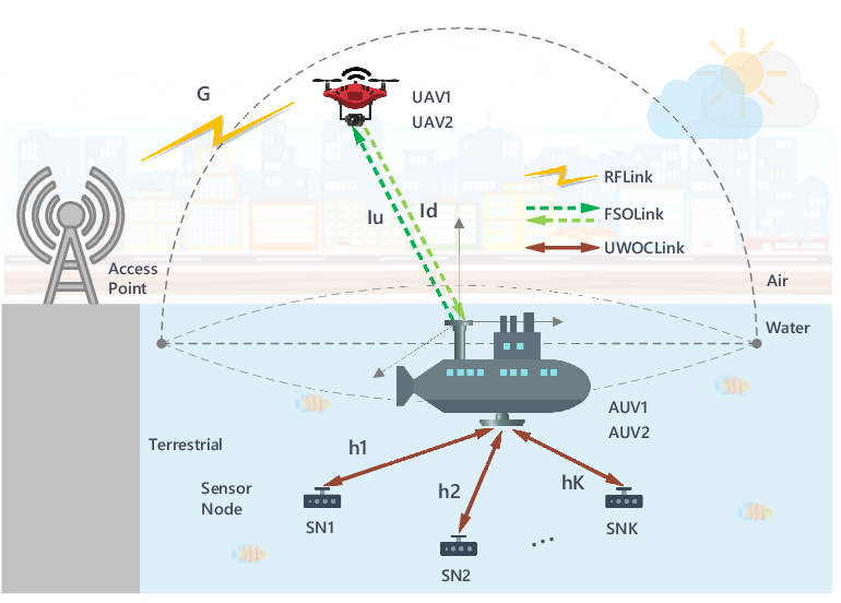
We assume a triple-hop UWSN in which $K$ SNs are connected to an AUV through UWOC links, the AUV is connected to a UAV via FSO links, and the UAV is connected to a terrestrial wireless AP with an RF link, c.f. Fig. 1. For the proposed system model, the following assumptions are made.

•

The UWOC and FSO links are deployed based on the wavelength-division multiplexing (WDM) technique.
•

The uplink and downlink transmissions over the UWOC and RF links are established under the time-division duplexing (TDD) scheme.
•

Two strategies are assumed for the FSO FD transmissions; direct transmission strategy (DTS) and retro-reflection strategy (RRS). In the DTS, uplink and downlink transmissions are performed over independent links. However, in the RRS, the uplink transmission is performed by reflecting the received downlink FSO beams on the UAV by an MRR terminal at the AUV.
•

On-off keying (OOK) modulation is applied for the uplink and downlink transmissions through all nodes.

It is also assumed that uplink and downlink data transmissions between the SNs and the AP are accomplished within $L$ time slots. In the case of TDD transmission, each slot with the length of $\tau$ is divided into uplink transmission (UT) and downlink transmission (DT) sub-slots with the lengths of $\tau_{u}$ and $\tau_{d}\!=\!\tau\!-\!\tau_{u}$ , respectively, c.f. Fig. 2. For an end-to-end connection between $K$ SNs and the AP, we have the following transmission framework.

Connection establishment. To establish the connection, the AUV and UAV relays transmit paging signals to their connected ends and synchronize them through a header slot (HS) with the length of $\tau_{\text{HS}}$ .

$L$ -slot data transmission. After the HS, the SNs and AP transmit their uplink and downlink information signals, respectively, in their dedicated sub-slots. Once each relay detects the signals, it demodulates, buffers, and forwards (DBF) the remodulated signals over the next time slot.

Connection termination. Finally, after $L$ time slots, the relays transmit another paging signals in a trailer slot (TS) with the length of $\tau_{\text{TS}}$ to terminate the connection.

Refer to caption — Fig. 1: The proposed UAV-assisted UWSN with RF and optical wireless links.

Before analysing the end-to-end performance of the UWSN, in the following subsections, we provide UWOC, FSO, and RF channel models, SNR expressions, and their corresponding statistics.

II-A UWOC Channel Model

The UWOC link of the $k$ th SN is modeled by [37]

h_{k}=h_{l,k}h_{t,k}h_{p,k},~\text{for}~k=1,2,...,K,

(1)

which includes the oceanic path-loss, $h_{l,k}$ , turbulence, $h_{t,k}$ , and pointing error, $h_{p,k}$ .

II-A1 Oceanic path-loss

$h_{l,k}$ is modeled under Beer-Lambert law, as below

h_{l,k}=\operatorname{exp}\!\left(-{\alpha_{a,k}d_{a,k}}\right)\!,

(2)

where $\alpha_{a,k}$ denotes the water extinction factor, and $d_{a,k}$ represents the average distance between the $k$ th SN and the AUV.

II-A2 Oceanic turbulence

For the conventional weak turbulence conditions, $h_{t,k}$ is modeled by a log-normal RV with the following probability density function (p.d.f) [1]

f_{h_{t,k}}(h_{t,k})=\frac{1}{2h_{t,k}\sqrt{2\pi\sigma_{x_{k}}^{2}}}\operatorname{exp}\!\left(\!-\frac{\left(\ln(h_{t,k})-2\mu_{x_{k}}\right)^{2}}{8\sigma_{x_{k}}^{2}}\right)\!\!,

(3)

such that $\mu_{x_{k}}\!=\!-\sigma_{x_{k}}^{2}$ , and $\sigma_{x_{k}}^{2}\!=\!0.307C_{n}^{2}k_{k}^{7/6}d_{a,k}^{11/6}$ , where $C_{n}^{2}$ represents the index of the refraction structure, $k_{k}\!=\!{2\pi}/\lambda_{k}$ is the optical wave number, and $\lambda_{k}$ denotes the wavelength of the $k$ th WDM channel.

II-A3 Oceanic pointing error

The p.d.f of $h_{p,k}$ for a circular detection mechanism is modeled by [5, 39]

f_{h_{p,k}}(h_{p,k})=\frac{\xi^{2}}{h_{0}^{\xi^{2}}}h_{p,k}^{\xi^{2}-1},~~0\leq h_{p,k}\leq h_{0},

(4)

where $h_{0}$ and $\xi$ are UWOC pointing error constants.

II-A4 Statistics of the UWOC link

By using (2)–(4) and similar steps as [40], the p.d.f of $h_{k}$ is derived as

f_{h_{k}}(h_{k})=\frac{\xi^{2}h_{k}^{\xi^{2}-1}}{2(h_{0}h_{l,k})^{\xi^{2}}}\operatorname{erfc}\!\left(\!\frac{\ln\!\left(\!{\frac{h_{k}}{h_{0}h_{l,k}}}\!\right)+\varphi_{k}}{\sqrt{8\sigma_{x_{k}}^{2}}}\!\right)\!\varphi_{k}^{\prime},

(5)

where $\varphi_{k}\!=\!2\sigma_{x_{k}}^{2}\!\left(1+2\xi^{2}\right)$ , and $\varphi_{k}^{\prime}\!=\!2\sigma_{x_{k}}^{2}\xi^{2}\!\left(1+\xi^{2}\right)$ .

Therefore, the received signal transmitted over the $k$ th UWOC link is written as

r_{k}=\eta_{k}h_{k}s_{k}+n_{k},

(6)

where $\eta_{k}$ denotes the optical-to-electrical conversion parameter, $s_{k}\!\in\!\{0,\sqrt{P}\}$ is the OOK modulation symbol, $P$ denotes the maximum transmission power, and $n_{k}\!\sim\!\mathcal{N}(0,\delta_{k}^{2})$ indicates the additive noise. Thus, the SNR of the $k$ th UWOC link is derived as

\gamma_{k}=\frac{\left(\eta_{k}h_{k}s_{k}\right)^{2}}{\delta_{k}^{2}}=\bar{\gamma}_{k}h_{k}^{2},

(7)

where $\bar{\gamma}_{k}={\eta_{k}^{2}s_{k}^{2}}/{\delta_{k}^{2}}$ represents the average SNR. By the use of (5) and (7), the p.d.f of $\gamma_{k}$ is obtained as

f_{\gamma_{k}}(\gamma_{k})=\frac{\xi^{2}\left(\gamma_{k}/\bar{\gamma}_{k}\right)^{\frac{\xi^{2}}{2}-1}}{4(h_{0}h_{l,k})^{\xi^{2}}}\operatorname{erfc}\!\left(\!\frac{\ln\!\left(\!{\frac{\sqrt{\gamma_{k}}}{h_{0}h_{l,k}\sqrt{\bar{\gamma}_{k}}}}\!\right)+\varphi_{k}}{\sqrt{8\sigma_{x_{k}}^{2}}}\!\right)\!\varphi_{k}^{\prime}.

(8)

By the use of the standard CDF definition, and after some mathematical manipulations, the CDF of $\gamma_{k}$ is derived as

		$\displaystyle F_{\gamma_{k}}(\gamma_{k})=\frac{\bar{\gamma}_{k}\varphi_{k}^{\prime}}{2}\Bigg[\!\operatorname{erfc}\!\left(\frac{\Theta_{k}(\gamma_{k})}{\sqrt{8\sigma_{x_{k}}^{2}}}\right)\!\operatorname{exp}\!\Big({{\Theta_{k}(\gamma_{k})\xi^{2}}}\Big)$
		$\displaystyle~~~+\operatorname{erfc}\!\left(\frac{4\sigma_{x_{k}}^{2}\xi^{2}-\Theta_{k}(\gamma_{k})}{\sqrt{8\sigma_{x_{k}}^{2}}}\right)\!\operatorname{exp}\!\Big(2\sigma_{x_{k}}^{2}\xi^{4}\Big)\!\Bigg]\!\operatorname{exp}\!\Big(\!\!-\varphi_{k}\xi^{2}\Big)\!,$		(9)

where $\Theta_{k}(\gamma_{k})=\ln\!\left(\!{\frac{\sqrt{\gamma_{k}}}{h_{0}h_{l,k}\sqrt{\bar{\gamma}_{k}}}}\!\right)+\varphi_{k}.$

II-B FSO Channel Model

The AUV–UAV FSO links experience W2A and A2W impacts caused by the erratic random and non-random waves in the air-water interface at the uplink and downlink transmissions, respectively. Specifically, the waves reflect and scatter optical signals and result in extra additive loss component which can exceed the absorption loss. Therefore, the FSO channel is modeled as

I_{j}=I_{l,j}I_{t,j}I_{p,j},

(10)

where $j\!=\!1$ stands for the downlink transmission, while $j\!=\!2$ indicates the uplink one. Also, $I_{l,j}$ , $I_{t,j}$ , and $I_{p,j}$ denote the atmospheric path-loss, turbulence, and pointing error, respectively.

II-B1 Atmospheric path-loss

$I_{l,j}$ is given by

I_{l,j}=\operatorname{exp}\!\left(-\alpha_{au}d_{au}\right)\!,

(11)

where $\alpha_{au}$ is the air attenuation factor which depends on weather conditions, and $d_{au}$ denotes the average distance between the AUV and UAV.

II-B2 Atmospheric turbulence

By taking into account the A2W and W2A impacts, $I_{t,j}$ follows the Birnbaum-Saunders distribution with the following p.d.f[37, 38]

	$\displaystyle f_{I_{t,j}}(I_{t,j};\alpha,\beta)$	$\displaystyle=\frac{1}{2\sqrt{2\pi}\alpha\beta}\left[\left(\frac{\beta}{I_{t,j}}\right)^{\!\!1/2}\!+\left(\frac{\beta}{I_{t,j}}\right)^{\!\!3/2}\right]$
		$\displaystyle~~~\times\operatorname{exp}\!\left[-\frac{1}{2\alpha^{2}}\left(\frac{I_{t,j}}{\beta}+\frac{\beta}{I_{t,j}}-2\right)\right]\!,$		(12)

where $\alpha\!>\!0$ and $\beta\!>\!0$ denote shape and scale parameters, respectively.

II-B3 Atmospheric pointing error

For $I_{p,j}$ , we have

f_{I_{p,j}}(I_{p,j})=\frac{\zeta^{2}}{I_{0}^{\zeta^{2}}}I_{p,j}^{\zeta^{2}-1},~~0\leq I_{p,j}\leq I_{0},

(13)

where $I_{0}\!=\!\left[\operatorname{erf}(\nu)\right]^{2}$ , and $\zeta\!=\!\frac{1}{2}w_{z_{eq}}\sigma_{s}^{-1}$ denotes the ratio between the equivalent beam radius and FSO pointing error displacement standard deviation. Also, $w_{z_{eq}}^{2}\!=\!w_{z}^{2}\sqrt{0.25\pi}\operatorname{erf}(\nu)\nu^{-1}\operatorname{exp}(\nu^{2})$ , and $\nu\!=\!\sqrt{0.5\pi}\,w_{z}^{-1}r_{s}$ , where $w_{z}$ denotes FSO beam waist at distance $z$ , and $r_{s}$ implies the alignment-based radial distance at the detector.

In the following two subsections, statistics of the FSO link are separately investigated for the DTS and RRS schemes.

II-B4 Statistics of the FSO link for the DTS

In the DTS, the signals are transmitted over two independent links in the uplink and downlink. Thus, the statistical properties of those links are studied in what follows.

Proposition 1.

The p.d.f of the FSO link for the DTS scheme is given by

	$\displaystyle f_{I_{j}}(I_{j};\alpha,\beta)$	$\displaystyle=\frac{e^{1/{\alpha^{2}}}}{2\sqrt{\pi}}\frac{\zeta^{2}I_{j}^{\zeta^{2}-1}}{\gamma_{0,j}^{\zeta^{2}}}\Bigg[\Gamma\!\left(\frac{1}{2}-\zeta^{2},\frac{I_{j}}{\gamma_{0,j}}\right)$
		$\displaystyle~~~+\frac{1}{2\alpha^{2}}\,\Gamma\!\left(\!-\frac{1}{2}-\zeta^{2},\frac{I_{j}}{\gamma_{0,j}}\right)\!\Bigg],$		(14)

where $\gamma_{0,j}\!=\!2\alpha^{2}\beta I_{0}I_{l,j}$ .

Sketch of Proof.

See Appendix A. ∎

In the DTS, the received FSO signals in the downlink, i.e., $j\!=\!1$ , and uplink, i.e., $j\!=\!2$ , are given by

\hat{\bm{r}}_{j}=\mu_{j}I_{j}\hat{\bm{s}}_{j}+\bm{w}_{j},

(15)

where $\hat{\bm{s}}_{j}\!=\!\left[\hat{s}_{j,1},\hat{s}_{j,2},...,\hat{s}_{j,K}\right]^{T}$ , $\hat{s}_{j,k}\!\in\!\{0,\sqrt{\hat{P}_{j}}\}$ is the information symbol with OOK modulation, and $\mathbb{E}\!\left\{\hat{s}_{j,k}\hat{s}_{j,k^{\prime}}\right\}\!=\!0$ for $k\!\neq\!k^{\prime}$ . Also, $\mu_{j}$ indicates the optical-to-electrical conversion parameter, and $\bm{w}_{j}\!\sim\!\mathcal{N}(\bm{0},\Phi_{j}^{2}I_{\!K\!\times\!K}\!)$ denotes the independent and identically distributed (i.i.d.) additive noise. Thus, the SNR for the $k$ th SN is as follows

\hat{{\gamma}}_{j,k}=\frac{\mu_{j}^{2}I_{j}^{2}\hat{{s}}_{j,k}^{2}}{{\Phi_{j}^{2}}}=\tilde{{\gamma}}_{j,k}I_{j}^{2},

(16)

where $\mathbb{E}\!\left\{\hat{{s}}_{j,k}{w}_{j,k}\right\}\!=\!{0}$ , and $\tilde{{\gamma}}_{j,k}\!=\!\mu_{j}^{2}\hat{{s}}_{j,k}^{2}/\Phi_{j}^{2}$ . By using (1) and (16), we have

		$\displaystyle f_{\hat{\gamma}_{j,k}}(\hat{\gamma}_{j,k};\alpha,\beta)=\frac{e^{1/{\alpha^{2}}}}{4\sqrt{\pi}}\frac{\zeta^{2}(\hat{\gamma}_{j,k}/\tilde{\gamma}_{j,k})^{\frac{\zeta^{2}}{2}-1}}{\gamma_{0,j}^{\zeta^{2}}}$
		$\displaystyle\!\!\times\!\Bigg[\Gamma\!\left(\frac{1}{2}-\zeta^{2},\frac{\sqrt{\hat{\gamma}_{j,k}}}{\gamma_{0,j}\sqrt{\tilde{\gamma}_{j,k}}}\right)+\frac{1}{2\alpha^{2}}\,\Gamma\!\left(\!-\frac{1}{2}-\zeta^{2},\frac{\sqrt{\hat{\gamma}_{j,k}}}{\gamma_{0,j}\sqrt{\tilde{\gamma}_{j,k}}}\right)\!\Bigg].\,$		(17)

By using the CDF definition and after some mathematical manipulations, the CDF of $\hat{\gamma}_{j,k}$ is derived as

		$\displaystyle F_{\hat{\gamma}_{j,k}}(\hat{\gamma}_{j,k};\alpha,\beta)=$
		$\displaystyle~~~~~\frac{2e^{1/{\alpha^{2}}}}{\sqrt{\pi}}\frac{\zeta^{2}\tilde{\gamma}_{j,k}^{1-\frac{\zeta^{2}}{2}}}{\gamma_{0,j}^{\zeta^{2}}(\zeta^{2}+6)}\Bigg[\!\Bigg(\!\Gamma\!\left(\frac{1}{2}-\zeta^{2},\frac{\sqrt{{\hat{\gamma}_{j,k}}}}{\gamma_{0,j}\sqrt{\tilde{\gamma}_{j,k}}}\right)$
		$\displaystyle~~~+\frac{1}{2\alpha^{2}}\Gamma\!\left(\!-\frac{1}{2}-\zeta^{2},\frac{\sqrt{{\hat{\gamma}_{j,k}}}}{\gamma_{0,j}\sqrt{\tilde{\gamma}_{j,k}}}\right)\!\Bigg)\hat{\gamma}_{j,k}^{\frac{\zeta^{2}+6}{8}}+\Big(\gamma_{0,j}\sqrt{\tilde{\gamma}_{j,k}}\Big)^{\!\!\frac{\zeta^{2}+6}{4}}$
		$\displaystyle\!\times\!\Bigg(\!\!\operatorname{\gamma}\!\left(\!2-\frac{3}{4}\zeta^{2},\frac{\sqrt{{\hat{\gamma}_{j,k}}}}{\gamma_{0,j}\sqrt{\tilde{\gamma}_{j,k}}}\right)\!+\!\frac{1}{2\alpha^{2}}\operatorname{\gamma}\!\left(\!1-\frac{3}{4}\zeta^{2},\frac{\sqrt{{\hat{\gamma}_{j,k}}}}{\gamma_{0,j}\sqrt{\tilde{\gamma}_{j,k}}}\right)\!\Bigg)\!\Bigg].\,$		(18)

II-B5 Statistics of the FSO link for the RRS

Thanks to the MRR system’s structure, the pointing error becomes negligible and is not taken into account in the RRS. Hence, for the downlink, by the use of (10)–(II-B2) with $j\!=\!1$ , we acquire

	$\displaystyle f_{I_{1}}(I_{1};\alpha,\beta)$	$\displaystyle=\frac{1}{2\sqrt{2\pi}\alpha\beta I_{l,1}}\left[\left(\frac{\beta I_{l,1}}{{I_{1}}}\right)^{\!\!1/2}\!+\left(\frac{\beta I_{l,1}}{{I_{1}}}\right)^{\!\!3/2}\right]$
		$\displaystyle~~~\times\operatorname{exp}\!\left[-\frac{1}{2\alpha^{2}}\left(\frac{{I_{1}}}{\beta I_{l,1}}+\frac{\beta I_{l,1}}{{I_{1}}}-2\right)\right]\!.$		(19)

Consequently, we have

		$\displaystyle f_{\hat{\gamma}_{1,k}}(\hat{\gamma}_{1,k};\alpha,\beta)=$
		$\displaystyle~~~\frac{1}{4\sqrt{2\pi}\alpha\beta I_{l,1}}\left[\left(\frac{\beta I_{l,1}\sqrt{\tilde{{\gamma}}_{1,k}}}{\sqrt{\hat{{\gamma}}_{1,k}}}\right)^{\!\!1/2}\!+\left(\frac{\beta I_{l,2}\sqrt{\tilde{{\gamma}}_{1,k}}}{\sqrt{\hat{{\gamma}}_{1,k}}}\right)^{\!\!3/2}\right]$
		$\displaystyle~~~\times\operatorname{exp}\!\left[-\frac{1}{2\alpha^{2}}\left(\frac{\sqrt{\hat{{\gamma}}_{1,k}}}{\beta I_{l,2}\sqrt{\tilde{{\gamma}}_{1,k}}}+\frac{\beta I_{l,2}\sqrt{\tilde{{\gamma}}_{1,k}}}{\sqrt{\hat{{\gamma}}_{1,k}}}-2\right)\right]\!.$		(20)

However, for the uplink, the received downlink signal at the AUV is reflected by the CCR and modulated by the MRR terminal, c.f. Fig. 3.

Therefore, the uplink signal at the UAV’s photodiode (PD) is given by¹¹ 1 Conventionally, the equivalent channel model for the RRS scheme is obtained by $I\!=\!I_{1}I_{2}$ with correlation coefficient $\rho$ . However, we assume that forward and backward channels are reciprocal, i.e., $\rho\!=\!1$ , so we have $I\!=\!I_{1}^{2}\!=\!I_{2}^{2}$ .

\hat{\bm{r}}_{2}=R\mu_{2}I_{2}^{2}\bm{x}_{m}\hat{\bm{s}}_{1}+\bm{w}_{2},

(21)

where $\bm{x}_{m}\!=\operatorname{diag}\left[x_{m,1},x_{m,2},...,x_{m,K}\right]$ is the i.i.d. modulated signal matrix at the MRR with $x_{m,k}\!\in\!\{0,1\}$ for the $k$ th SN with OOK modulation. Also, $R$ denotes the reflection effect of the CCR²² 2 For the proposed FSO system, parameter $R$ is equivalent to a geometric loss at the AUV–UAV link, which has the formula as in [34, (14)].. Therefore, we have

	$\displaystyle f_{I_{2}}(I_{2};\alpha,\beta)$	$\displaystyle=\frac{I_{2}^{-1/2}}{4\sqrt{2\pi}\alpha\beta I_{l,2}}\left[\left(\frac{\beta I_{l,2}}{\sqrt{I_{2}}}\right)^{\!\!1/2}\!+\left(\frac{\beta I_{l,2}}{\sqrt{I_{2}}}\right)^{\!\!3/2}\right]$
		$\displaystyle~~~\times\operatorname{exp}\!\left[-\frac{1}{2\alpha^{2}}\left(\frac{\sqrt{I_{2}}}{\beta I_{l,2}}+\frac{\beta I_{l,2}}{\sqrt{I_{2}}}-2\right)\right]\!.~$		(22)

The SNR’s diagonal matrix in the uplink is derived as

\hat{{\gamma}}_{2,k}=\frac{R^{2}\mu_{2}^{2}I_{2}^{4}{x}_{m,k}^{2}\hat{s}_{2,k}^{2}}{\Phi_{2}^{2}}=\tilde{{\gamma}}_{2,k}I_{2}^{4},

(23)

where $\tilde{{\gamma}}_{2,k}=R^{2}\mu_{2}^{2}{x}_{m,k}^{2}\hat{{s}}_{2,k}^{2}/{\Phi_{2}^{2}}$ . As a result, we obtain

		$\displaystyle\!\!\!f_{\hat{\gamma}_{2,k}}(\hat{\gamma}_{2,k};\alpha,\beta)=$
		$\displaystyle\!\!\!\frac{\sqrt{\tilde{{\gamma}}_{2,k}}}{8\sqrt{2\pi}\alpha\beta I_{l,2}\sqrt{\hat{{\gamma}}_{2,k}}}\left[\left(\frac{\beta I_{l,2}\sqrt[4]{\tilde{{\gamma}}_{2,k}}}{\sqrt[4]{\hat{{\gamma}}_{2,k}}}\right)^{\!\!1/2}\!\!+\left(\frac{\beta I_{l,2}\sqrt[4]{\tilde{{\gamma}}_{2,k}}}{\sqrt[4]{\hat{{\gamma}}_{2,k}}}\right)^{\!\!3/2}\right]$
		$\displaystyle~\!\times\operatorname{exp}\!\left[-\frac{1}{2\alpha^{2}}\left(\frac{\sqrt[4]{\hat{{\gamma}}_{2,k}}}{\beta I_{l,2}\sqrt[4]{\tilde{{\gamma}}_{2,k}}}+\frac{\beta I_{l,2}\sqrt[4]{\tilde{{\gamma}}_{2,k}}}{\sqrt[4]{\hat{{\gamma}}_{2,k}}}-2\right)\right]\!.~$		(24)

By using (II-B5) and (II-B5), the CDF of $\hat{\gamma}_{j,k}$ for the RRS scheme is derived as

		$\displaystyle F_{\hat{\gamma}_{j,k}}(\hat{\gamma}_{j,k};\alpha,\beta)=$
		$\displaystyle~~~\operatorname{\Phi}\!\Bigg(\frac{1}{\alpha}\Bigg[\bigg(\frac{\sqrt[2j]{\hat{{\gamma}}_{j,k}}}{\beta I_{l,j}\sqrt[2j]{\tilde{{\gamma}}_{j,k}}}\bigg)^{\!\!1/2}\!\!-\bigg(\frac{\beta I_{l,j}\sqrt[2j]{\tilde{{\gamma}}_{j,k}}}{\sqrt[2j]{\hat{{\gamma}}_{j,k}}}\bigg)^{\!\!1/2}\Bigg]\Bigg).$		(25)

II-C RF Channel Model

The RF link between the UAV and the terrestrial AP is modeled by

G=G_{l}^{1/2}G_{s},

(26)

where $G_{l}$ and $G_{s}$ denote the large- and small-scale fading, respectively.

II-C1 Large-scale fading

The large-scale fading consists of the pathloss and shadowing, as follows [41]

G_{l}=-20\log_{10}\!\left(\!\frac{40\pi}{3}f\!\right)\!-\!27\log_{10}(d_{ut})\!+\!\chi_{sh}\,[\text{dB}],

(27)

where $f$ $[\text{GHz}]$ is the RF frequency, $d_{ut}$ $[\text{m}]$ denotes the distance, and $\chi_{sh}\!\sim\!\mathcal{N}(0,\sigma_{sh}^{2})$ presents the shadowing.

II-C2 Small-scale fading

$G_{s}$ follows the Nakagami- $m$ distribution with the following p.d.f [6]

f_{G_{s}}(G_{s};m)=\frac{2m^{m}G_{s}^{2m-1}}{\Gamma(m)\Omega^{m}}\operatorname{exp}\!\left(\!-\frac{mG_{s}^{2}}{\Omega}\right)\!,

(28)

where $\Omega\!=\!\mathbb{E}\!\left\{G_{s}^{2}\right\}$ , and $0.5\!\leq\!m\!\leq\!\infty$ indicates the Nakagami fading parameter.

The received RF signal is given by

\hat{\vphantom{\rule{1.0pt}{6.36115pt}}\smash{\hat{{\bm{r}}}}}=G\hat{\vphantom{\rule{1.0pt}{6.36115pt}}\smash{\hat{{\bm{s}}}}}+\bm{v},

(29)

where $\hat{\vphantom{\rule{1.0pt}{6.36115pt}}\smash{\hat{{\bm{s}}}}}\!=\!\left[\hat{\vphantom{\rule{1.0pt}{6.36115pt}}\smash{\hat{{s}}}}_{1},\hat{\vphantom{\rule{1.0pt}{6.36115pt}}\smash{\hat{{s}}}}_{2},...,\hat{\vphantom{\rule{1.0pt}{6.36115pt}}\smash{\hat{{s}}}}_{K}\right]^{T}$ , $\hat{\vphantom{\rule{1.0pt}{6.36115pt}}\smash{\hat{{s}}}}_{k}\!\in\!\{0,\sqrt{\hat{\vphantom{\rule{1.0pt}{6.36115pt}}\smash{\hat{{P}}}}}\}$ is the transmission symbol with OOK modulation, and $\mathbb{E}\!\left\{\hat{\vphantom{\rule{1.0pt}{6.36115pt}}\smash{\hat{{s}}}}_{k}\hat{\vphantom{\rule{1.0pt}{6.36115pt}}\smash{\hat{{s}}}}_{k^{\prime}}\right\}\!=\!0$ for $k\!\neq\!k^{\prime}$ . Also, $\bm{v}\!\sim\!\mathcal{CN}(\bm{0},\Lambda^{2}I_{\!K\!\times\!K}\!)$ is the i.i.d. additive noise. Hence, the SNR is obtained as

\hat{\vphantom{\rule{1.0pt}{6.36115pt}}\smash{\hat{\gamma}}}_{k}=\frac{G^{2}\hat{\vphantom{\rule{1.0pt}{6.36115pt}}\smash{\hat{s}}}_{k}^{2}}{\Lambda^{2}}=\tilde{\vphantom{\rule{1.0pt}{6.57643pt}}\smash{\tilde{\gamma}}}_{k}G^{2},

(30)

where $\tilde{\vphantom{\rule{1.0pt}{6.57643pt}}\smash{\tilde{\gamma}}}_{k}\!=\!\hat{\vphantom{\rule{1.0pt}{6.36115pt}}\smash{\hat{s}}}_{k}^{2}/\Lambda^{2}$ . By the use of (28) and (30), we have

f_{\hat{\hat{\gamma}}_{k}}(\hat{\vphantom{\rule{1.0pt}{6.36115pt}}\smash{\hat{{\gamma}}}}_{k};m)=\frac{m^{m}{\hat{\vphantom{\rule{1.0pt}{6.36115pt}}\smash{\hat{{\gamma}}}}}_{k}^{m-1}}{\Gamma(m)\tilde{\vphantom{\rule{1.0pt}{6.57643pt}}\smash{\tilde{{\gamma}}}}_{k}^{m}G_{l}^{m}}\operatorname{exp}\!\left(\!-\frac{m\hat{\vphantom{\rule{1.0pt}{6.36115pt}}\smash{\hat{{\gamma}}}}_{k}}{\tilde{\vphantom{\rule{1.0pt}{6.57643pt}}\smash{\tilde{{\gamma}}}}_{k}G_{l}}\!\right)\!.

(31)

Consequently, the CDF of $\hat{\vphantom{\rule{1.0pt}{6.36115pt}}\smash{\hat{{\gamma}}}}_{k}$ is given by

F_{\hat{\hat{\gamma}}_{k}}(\hat{\vphantom{\rule{1.0pt}{6.36115pt}}\smash{\hat{{\gamma}}}}_{k};m)=\frac{1}{\Gamma(m)}\operatorname{\gamma}\!\left(\!m,\frac{m\hat{\vphantom{\rule{1.0pt}{6.36115pt}}\smash{\hat{{\gamma}}}}_{k}}{\tilde{\vphantom{\rule{1.0pt}{6.57643pt}}\smash{\tilde{{\gamma}}}}_{k}G_{l}}\!\right)\!.

(32)

III AUV–UAV Tracking Procedure and Performance Analyses

In this section, we firstly propose an AUV–UAV tracking procedure, and then the end-to-end outage probability and average BER expressions are derived.

III-A AUV–UAV Tracking Procedure

To set up reliable and stable FSO communications between the AUV and the UAV, a tracking procedure is required. To this end, we propose Algorithm 1, i.e., an $n$ -step acquisition-and-tracking algorithm applied at the UAV, wherein two tracking modes are considered; coarse and fine tracking modes [33]. Despite trying to provide LOS light paths between the AUV and the UAV in the coarse tracking mode, non-negligible tracking and pointing errors may remain. The fine tracking mode is also considered to fix this issue and make the tracking more accurate.

•

In the coarse tracking mode, based on the light detection and ranging (LiDAR) technology, the UAV persistently transmits short but energetic pulses to catches the AUV and track its trajectory by measuring the reflected signals. Afterward, a gimbal tracker at the UAV sweeps the AUV’s surface to find its optical lens and align the FSO links between the relays, c.f. Fig. 3.
•

In the fine tracking mode, the AUV transmits beacon signals to the UAV after detecting the tracking pulses. Then, at the UAV, the beacon signals are measured by a quadrant photodiode (QPD) and used for driving a fast steering mirror (FSM) under a step track algorithm [42], c.f. Fig. 3.

As depicted in Fig. 4, the measured FSO beam at four quadrants of the QPD are denoted by $\vartheta_{1}$ , $\vartheta_{2}$ , $\vartheta_{3}$ , and $\vartheta_{4}$ , thus the tracking errors are calculated as [42]


$\displaystyle e_{x}$	$\displaystyle=\left\|\frac{(\vartheta_{1}+\vartheta_{4})-(\vartheta_{2}+\vartheta_{3})}{\vartheta_{1}+\vartheta_{2}+\vartheta_{3}+\vartheta_{4}}\right\|,$	(33a)
$\displaystyle e_{y}$	$\displaystyle=\left\|\frac{(\vartheta_{1}+\vartheta_{2})-(\vartheta_{3}+\vartheta_{4})}{\vartheta_{1}+\vartheta_{2}+\vartheta_{3}+\vartheta_{4}}\right\|.$	(33b)

The aim is to achieve almost perfect alignment, i.e., $(e_{x},e_{y})\!\cong\!(0,0)$ . However, it is more practical to define thresholds, such as $\varepsilon_{x}$ and $\varepsilon_{y}$ , for indicating alignment quality conditions. Once $e_{x}$ and $e_{y}$ individually meet $\varepsilon_{x}$ and $\varepsilon_{y}$ , the FSO connections between the AUV and the UAV relays will be established and continued.

Input: Angle parameters

\psi_{j}

\psi_{\text{min}}

\psi_{\text{max}}

, and

\Delta\psi

; the FSO beam at the QPD’s quadrants

\vartheta_{1}

\vartheta_{2}

\vartheta_{3}

, and

\vartheta_{4}

; QPD sampling size

A_{\text{QPD}}

; thresholds

\varepsilon_{x}

and

\varepsilon_{y}

; step factors

n_{0}

and

n

Catch the AUV by using the LiDAR technology.
Initiate

i\!=\!0

.
while the AUV’s beacon signals are not detected do 1

Coarse tracking:
Set the UAV’s divergence angle to

\psi_{j}\!=\!\psi_{\text{min}}\!+\!i\Delta\psi

.
if $\psi_{j}\!=\!\psi_{\text{max}}$ then go to 2;

else

i\!=\!i\!+\!1

. 2

Set

n_{0}\!=\!i

.
Initiate

i\!=\!0

.
Compute

(e_{x},e_{y})

\vartheta_{1}

\vartheta_{2}

\vartheta_{3}

\vartheta_{4}

, (33a), and (33b).
for $i\!\leftarrow\!0$ to $A_{\text{{QPD}}}\!-\!1$ do 3

Fine tracking:
if $(e_{x},e_{y})\!\leq\!(\varepsilon_{x},\varepsilon_{y})$ then set

n\!=\!i\!+\!n_{0}

; stop the process;

else adjust the UAV’s FSM for the

i

th tracking step; update

(e_{x},e_{y})

. 4

Go to 2.

Algorithm 1 The

n

-step tracking procedure

III-B Outage Probability

The end-to-end SNR for the $k$ th SN in the downlink, i.e., $j\!=\!1$ , and uplink, i.e., $j\!=\!2$ , is defined as $\gamma_{j,k}\!=\!\operatorname{min}\!\big\{\!\gamma_{k},\hat{\gamma}_{j,k},\hat{\vphantom{\rule{1.0pt}{6.36115pt}}\smash{\hat{{\gamma}}}}_{k}\!\big\}$ . Herein, $\gamma_{k}$ , $\hat{\gamma}_{j,k}$ , and $\hat{\vphantom{\rule{1.0pt}{6.36115pt}}\smash{\hat{{\gamma}}}}_{k}$ are the SNRs of the UWOC, FSO, and RF links, which are previously presented in (7), (16) or (23), and (30). Therefore, the CDF of $\gamma_{j,k}$ is computed as [43]

		$\displaystyle F_{\gamma_{j,k}}(\gamma_{j,k};\alpha,\beta,m)=F_{\gamma_{k}}(\gamma_{j,k})\!+\!F_{\hat{\gamma}_{j,k}}(\gamma_{j,k};\alpha,\beta)$
		$\displaystyle~~~~~+\!F_{\hat{\hat{\gamma}}_{k}}(\gamma_{j,k};m)\!-\!F_{\gamma_{k}}(\gamma_{j,k})F_{\hat{\gamma}_{j,k}}(\gamma_{j,k};\alpha,\beta)$
		$\displaystyle~~~~~-\!F_{\hat{\gamma}_{j,k}}(\gamma_{j,k};\alpha,\beta)F_{\hat{\hat{\gamma}}_{k}}(\gamma_{j,k};m)\!-\!F_{\gamma_{k}}(\gamma_{j,k})F_{\hat{\hat{\gamma}}_{k}}(\gamma_{j,k};m)$
		$\displaystyle~~~~~+F_{\gamma_{k}}(\gamma_{j,k})F_{\hat{\gamma}_{j,k}}(\gamma_{j,k};\alpha,\beta)F_{\hat{\hat{\gamma}}_{k}}(\gamma_{j,k};m)$
		$\displaystyle=1\!-\!\Big(\!1\!-\!F_{\gamma_{k}}(\gamma_{j,k})\!\Big)\Big(\!1\!-\!F_{\hat{\gamma}_{j,k}}(\gamma_{j,k};\alpha,\beta)\!\Big)\Big(\!1\!-\!F_{\hat{\hat{\gamma}}_{k}}(\gamma_{j,k};m)\!\Big).$		(34)

The quality of service (QoS) is ensured by keeping $\gamma_{j,k}$ above a given threshold $\gamma_{th}$ . Thus, the outage probability for the $k$ th SN is defined as

\displaystyle P_{out,j,k}(\alpha,\beta,m)\triangleq\operatorname{Pr}\!\left\{\gamma_{j,k}\leq\gamma_{th}\right\}=F_{\gamma_{j,k}}(\gamma_{th};\alpha,\beta,m).

(35)

By using (III-B) and (35), we have

		$\displaystyle P_{out,j,k}(\alpha,\beta,m)=1\!-\!\Big(\!1\!-\!F_{\gamma_{k}}(\gamma_{th})\!\Big)$
		$\displaystyle~~~~~~~~\times\!\Big(\!1\!-\!F_{\hat{\gamma}_{j,k}}(\gamma_{th};\alpha,\beta)\!\Big)\Big(\!1\!-\!F_{\hat{\hat{\gamma}}_{k}}(\gamma_{th};m)\!\Big).$		(36)

III-C Average Bit Error Rate

As well-known, the bit error probability at each hop becomes independent from that of the other link according to the DBF protocol. Hence, the end-to-end average BER for the $k$ th SN in the downlink, i.e., $j\!=\!1$ , and uplink, i.e., $j\!=\!2$ , is derived as

		$\displaystyle P_{e,j,k}(\alpha,\beta,m)=$
		$\displaystyle~~~~~~1\!-\!\Big(\!1\!-\!P_{e_{1},k}\!\Big)\Big(\!1\!-\!P_{e_{2},j,k}(\alpha,\beta)\!\Big)\Big(\!1\!-\!P_{e_{3},k}(m)\!\Big),$		(37)

where $P_{e_{1},k}$ , $P_{e_{2},j,k}(\alpha,\beta)$ , and $P_{e_{3},k}$ respectively denote the average BERs of the SN–AUV, AUV–UAV, and UAV–AP links, which have the following expressions.

$\displaystyle P_{e_{1},k}$	$\displaystyle=\frac{q^{p}}{2\Gamma(p)}\int_{0}^{\infty}e^{-q\gamma}\gamma^{p-1}F_{{\gamma}_{k}}(\gamma)\,d\gamma$
	$\displaystyle=\frac{q^{p}\bar{\gamma}_{k}\varphi_{k}^{\prime}}{2\Gamma(p)}\operatorname{exp}\!\big(\!-\!\varphi_{k}\xi^{2}\big)\Bigg[2\operatorname{exp}\!\Big(-\frac{c_{1}(8\sigma_{x_{k}}^{2}\xi^{2}+c_{1})}{8\sigma_{x_{k}}^{2}}\Big)$
	$\displaystyle\times\!\Bigg(\dfrac{\operatorname{exp}\!\Big(\big(8\sigma_{x_{k}}^{2}(\xi^{2}+2p)+2c_{1}\big)^{2}/{32\sigma_{x_{k}}^{2}}\Big)}{\xi^{2}+2p}$
	$\displaystyle-\dfrac{\operatorname{exp}\!\Big(\big(8\sigma_{x_{k}}^{2}(\xi^{2}+2p+2)+2c_{1}\big)^{2}/{32\sigma_{x_{k}}^{2}}\Big)}{\xi^{2}+2p+2}\Bigg)$
	$\displaystyle+\operatorname{exp}\!\Big(2\sigma_{x_{k}}^{2}\xi^{4}\Big)\!\Bigg(\dfrac{\operatorname{exp}\!\Big((p+1)\big(8\sigma_{x_{k}}^{2}(p+1)+2c_{2}\big)\Big)}{p+1}$
	$\displaystyle-\dfrac{\operatorname{exp}\!\Big(p\big(8\sigma_{x_{k}}^{2}p+2c_{2}\big)\Big)}{p}\Bigg)\Bigg],$	(38)

where $c_{1}\!=\!\ln\!\big({{h_{0}h_{l,k}\sqrt{\bar{\gamma}_{k}}}}\big)\!-\!\varphi_{k}$ , and $c_{2}\!=\!c_{1}\!+{4\sigma_{x_{k}}^{2}}\xi^{2}$ . However, $P_{e_{2},j,k}(\alpha,\beta)$ is computed separately for the DTS and RRS schemes. Hence, in the DTS, we have

$\displaystyle P_{e_{2},j,k}(\alpha,\beta)$	$\displaystyle=\frac{q^{p}}{2\Gamma(p)}\!\int_{0}^{\infty}\!\!e^{-q\gamma}\gamma^{p-1}F_{\hat{\gamma}_{j,k}}(\gamma;\alpha,\beta)\,d\gamma$
	$\displaystyle\hskip-34.14322pt=\frac{q^{p}e^{1/{\alpha^{2}}}}{\sqrt{\pi}\Gamma(p)}\frac{\zeta^{2}\tilde{\gamma}_{j,k}({\gamma_{0,j}^{2}\tilde{\gamma}_{j,k}})^{-\frac{\zeta^{2}}{2}+p+1}}{(\zeta^{2}+6)}\Bigg[(\gamma_{0,j}^{2}{\tilde{\gamma}_{j,k}})^{q}$
	$\displaystyle\hskip-34.14322pt\times\!\bigg(\!-\frac{\Gamma(-\xi^{2}+2c_{3}+\frac{9}{2})}{c_{3}+2}-\frac{\Gamma(-\xi^{2}+2c_{3}+\frac{7}{2})}{2\alpha^{2}(c_{3}+2)}$
	$\displaystyle\hskip-34.14322pt+\frac{\Gamma(-\frac{3}{4}\xi^{2}+2p+4)}{p+1}-\frac{\Gamma(-\frac{3}{4}\xi^{2}+2p+3)}{2\alpha^{2}(p+1)}\bigg)$
	$\displaystyle\hskip-34.14322pt+\bigg(\frac{\Gamma(-\xi^{2}+2c_{3}+\frac{5}{2})}{c_{3}+1}+\frac{\Gamma(-\xi^{2}+2c_{3}+\frac{3}{2})}{2\alpha^{2}(c_{3}+1)}$
	$\displaystyle\hskip-34.14322pt-\frac{\Gamma(-\frac{3}{4}\xi^{2}+2p+2)}{p}+\frac{\Gamma(-\frac{3}{4}\xi^{2}+2p+1)}{2\alpha^{2}p}\bigg)\Bigg],$	(39)

where $c_{3}\!=\!\frac{\zeta^{2}-2}{8}\!+\!p$ , and in the RRS, we have

		$\displaystyle P_{e_{2},j,k}(\alpha,\beta)=\frac{q^{p}}{2\Gamma(p)}\!\int_{0}^{\infty}\!\!\!\!e^{-q\gamma}\gamma^{p-1}F_{\hat{\gamma}_{j,k}}(\gamma;\alpha,\beta)\,d\gamma$
		$\displaystyle=\frac{q^{p}}{4\Gamma(p)}\!\int_{0}^{\infty}\!e^{-q\gamma}\gamma^{p-1}\operatorname{erfc}\!\Bigg(\!\!\frac{1}{\alpha\sqrt{2}}\Bigg[\!\bigg(\frac{\sqrt[2j]{{{\gamma}}}}{\beta I_{l,j}\sqrt[2j]{\tilde{{\gamma}}_{j,k}}}\bigg)^{\!\!1/2}$
		$\displaystyle~~~-\bigg(\frac{\beta I_{l,j}\sqrt[2j]{\tilde{{\gamma}}_{j,k}}}{\sqrt[2j]{{{\gamma}}}}\bigg)^{\!\!1/2}\Bigg]\Bigg)d\gamma$
		$\displaystyle\simeq\frac{q^{p}}{4\Gamma(p)}\Bigg[\!-\left(\!{\alpha\sqrt{2\beta I_{l,j}\sqrt[2j]{\tilde{{\gamma}}_{j,k}}}}\right)^{\!4j(p+1)}\frac{\Gamma\!\left({2j(p+1)+\frac{1}{2}}\right)}{\sqrt{\pi}(p+1)}$
		$\displaystyle~~~+\left(\!{\alpha\sqrt{2\beta I_{l,j}\sqrt[2j]{\tilde{{\gamma}}_{j,k}}}}\right)^{\!4jp}\frac{\Gamma\!\left({2jp+\frac{1}{2}}\right)}{\sqrt{\pi}p}$
		$\displaystyle~~~+\left(\frac{1}{\alpha}\sqrt{\frac{\sqrt[2j]{\tilde{{\gamma}}_{j,k}}}{2\beta I_{l,j}}}\right)^{\!4j(p+1)}\frac{\Gamma\!\left({-2j(p+1)+\frac{1}{2}}\right)}{\sqrt{\pi}(p+1)}$
		$\displaystyle~~~-\left(\frac{1}{\alpha}\sqrt{\frac{\sqrt[2j]{\tilde{{\gamma}}_{j,k}}}{2\beta I_{l,j}}}\right)^{\!4jp}\frac{\Gamma\!\left({-2jp+\frac{1}{2}}\right)}{\sqrt{\pi}p}\Bigg].$		(40)

Also, we have

$\displaystyle P_{e_{3},k}(m)$	$\displaystyle=\frac{q^{p}}{2\Gamma(p)}\int_{0}^{\infty}e^{-q\gamma}\gamma^{p-1}F_{\hat{\hat{\gamma}}_{k}}(\gamma;m)\,d\gamma$
	$\displaystyle=\frac{q^{p}}{2\Gamma(p)\Gamma(m)}\int_{0}^{\infty}e^{-q\gamma}\gamma^{p-1}\operatorname{\gamma}\!\left(\!m,\frac{m\gamma}{\tilde{\vphantom{\rule{1.0pt}{6.57643pt}}\smash{\tilde{{\gamma}}}}_{k}}\!\right)d\gamma$
	$\displaystyle=\frac{q^{p}}{2\Gamma(p)\Gamma(m)}\bigg[{\left(\frac{\tilde{\vphantom{\rule{1.0pt}{6.57643pt}}\smash{\tilde{{\gamma}}}}_{k}}{m}\right)^{\!p+1}}\frac{\Gamma(m+p+1)}{p+1}$
	$\displaystyle~~~-{\left(\frac{\tilde{\vphantom{\rule{1.0pt}{6.57643pt}}\smash{\tilde{{\gamma}}}}_{k}}{m}\right)^{\!p}}\frac{\Gamma(m+p)}{p}\bigg].$	(41)

In (III-C)–(III-C), $p\!=\!0.5$ and $q\!=\!0.25$ with OOK modulation [5].

IV Numerical Results and Discussions

In what follows, the performance of the triple-hop UWSN is investigated through numerical results, from various perspectives. The wavelength assignments for the UWOC links are performed with the center wavelength of $532$ $\![\text{nm}]$ and grid size of $30$ $\![\text{mm}]$ , c.f. Fig. 5. Thus, the wavelength assigned to the $k$ th UWOC link, i.e., $\lambda_{k}$ , is

\dfrac{1}{\lambda_{k}}=\dfrac{1}{532}+\dfrac{(-1)^{k-1}}{30\!\times\!10^{6}}\Big\lceil\dfrac{k-1}{2}\Big\rceil.

(42)

The parameters used for the numerical results are summarized in Table I, otherwise they are clearly mentioned in the paper.

TABLE I: Network parameters for numerical results.

Parameter	Symbol	Value
FSO wavelengths	$\{\lambda_{u},\lambda_{d}\}$	$\{1064,1550\}$ $\![\text{nm}]$
RF frequency	$f$	$2$ $\![\text{GHz}]$
Average links’ lengths	$\{d_{a,k},d_{au},d_{ut}\}$	$\{0.15,1.5,20\}$ $\![\text{km}]\!\!$
Clear water extinction factor	$\alpha_{a,k}$	$21.79$ $\![\text{dB/km}]$
Clear air attenuation factor	$\alpha_{au}$	$0.44$ $\![\text{dB/km}]$
Snowy air attenuation factor		$4.53$ $\![\text{dB/km}]$
Foggy air attenuation factor		$50$ $\![\text{dB/km}]$
Refraction structure index	$C_{n}^{2}$	$10^{-15}$ $\![\text{m}^{-2/3}]$
UWOC pointing error constants	$\{h_{0},\xi\}$	$\{0.0764,2.35\}$
FSO displacement deviation	$\sigma_{s}$	$30$ $[\text{cm}]$
FSO beam waist	$w_{z}$	$1.25$ $[\text{m}]$
FSO receiver’s radius	$r_{a}$	$20$ $[\text{cm}]$
Birnbaum-Saunders parameters	$\{\alpha,\beta\}$	$\!\{0.6866,0.8093\}$
Shadowing standard deviation	$\sigma_{sh}$	$8$ $\![\text{dB}]$
Nakagami fading parameter	$m$	$0.5$
Reflection effect of the CCR	$R$	$0.5$

To investigate the network’s end-to-end outage probability and average BER, Fig. 6 (a) and Fig. 6 (b) are depicted, respectively. It is shown that the retro-reflection system improves the network’s outage probability and average BER, compared to the FSO direct transmission scheme. For example, the RRS scheme outperforms the DTS one in the uplink and downlink with on average $200\%$ ( $32\%$ ) and $80\%$ ( $17\%$ ) better outage probability (average BER), respectively, in the case of the clear weather and the average SNR of $40$ $\![\text{dB}]$ . This happens due to the fact that the pointing error is assumed negligible for the FSO links based on the retro-reflection system. The same reason is also true if we compare the RRS uplink with its downlink, where the primary one surpasses the latter one. As an illustrative example, for the clear weather and the average SNR of $40$ $\![\text{dB}]$ , the RRS uplink offers about $67\%$ ( $13\%$ ) lower outage probability (average BER) than the downlink one. In this case, since the uplink channel incorporates two correlated pointing error-free forward and backward channels, it presents a better performance compared to the downlink channel. Moreover, in both figures, the network’s performance is analyzed under clear, snowy, and foggy weather conditions. As expected, the network’s performance degrades by changing the weather from a clear condition to the foggy one. All results are verified by Monte-Carlo simulations with $500$ iterations.

Fig. 7 illustrates the AUV–UAV fine tracking procedure on a QPD with a $40\!\times\!40$ $\![\text{cm}^{2}]$ dimension, $2$ $\![\text{cm}]$ grid size, and $A_{\text{{QPD}}}\!=\!441$ sampling points. In this figure, a random $16$ -point dashed circle area within the defined dimension is assigned for the FSO beam refracted on the QPD after the coarse tracking procedure. Based on the step track algorithm, a tracking pointer starts from the center and sweeps the QPD’s surface step-by-step to find the location of the beam. Once the beam is tracked, the pointer tries to measure the beams’ territory. After the tracking procedure is successfully done, the FSM aligns the FSO beam to the center of the QPD and minimizes the tracking and pointing errors. Herein, the white, yellow (within the dashed circle area), and solid blue spots show sampling points, FSO beam, and tracking points, where each blue line connecting a tracking point to its neighbor is a tracking step.

Besides, Fig. 8 depicts the AUV-UAV tracking error, i.e., $e_{x}$ or $e_{y}$ , versus the number of tracking steps, based on a Monte-Carlo simulation with $500$ iterations. For the coarse tracking, we have $\psi_{\text{min}}\!=\!-\tan^{\!-1}(12.5/d_{au}[\text{m}])$ , $\psi_{\text{max}}\!=\!\tan^{\!-1}(12.5/d_{au}[\text{m}])$ , and $\Delta\psi\!=\!2\tan^{\!-1}(w_{z}/d_{au}[\text{m}])$ . Given that, if it is assumed that the AUV’s length is about $25$ $\![\text{m}]$ , the coarse tracking step would take an integer random value between $1$ and $10$ . In this figure, the coarse tracking is performed within almost $n_{0}\!=\!6$ steps. However, for the fine tracking, the procedure as depicted in Fig. 7 is simulated separately for $40\!\times\!40$ and $60\!\times\!60$ $\![\text{cm}^{2}]$ QPD dimensions, i.e., $A_{\text{{QPD}}}\!=\!441$ and $961$ with the grid size of $2$ $\![\text{cm}]$ , respectively, and the step sizes of $2$ and $4$ $\![\text{cm}]$ . It is concluded that there is a trade-off between the tracking error threshold and the number of tracking steps. The number of tracking steps reduces for larger step size, with the penalty of non-zero tracking error threshold. For instance, with $441$ sampling points and $2$ $\![\text{cm}]$ step size, the tracking error drops to zero with average $n\!=\!112$ steps. Nevertheless, with the same sampling points but $4$ $\![\text{cm}]$ step size, the tracking error diminishes to its minimum value of $0.11$ with average $n\!=\!67$ steps. Furthermore, it is shown that increasing the number of sampling points boosts the number of tracking steps, thus it takes much time to track the FSO beam on the QPD.

Fig. 9 (a) and Fig. 9 (b) sequentially present the network’s outage probability and average BER versus average SNR for different values of the tracking error threshold, i.e., $\varepsilon\!=\!\varepsilon_{x}\!=\!\varepsilon_{y}$ . According to Fig. 8, a minimum number of tracking steps is required based on the number of sampling points and the step size to meet the dedicated threshold. As an example, with $441$ sampling points and $2$ $[\text{cm}]$ step size, about $112$ , $109$ , and $100$ steps are required to satisfy $\varepsilon\!=\!0$ , $\varepsilon\!=\!0.1$ , and $\varepsilon\!=\!0.2$ , respectively. It is also observed that the RRS uplink outperforms the RRS downlink, and the RRS downlink outperforms both DTS uplink and downlink. It is shown that, by increasing the tracking error threshold, the network’s performance degrades since the tracking and pointing errors are enlarged. For instance, in the case of the clear weather with the average SNR of $40$ $\![\text{dB}]$ , the outage probability for the uplink RRS takes on average $20\%$ and $75\%$ higher values by increasing the threshold from $\varepsilon\!=\!0$ to $\varepsilon\!=\!0.1$ and $\varepsilon\!=\!0.2$ , respectively. For depicting this figure, we initiate $w_{z}^{-1}r_{s}$ as $0.84$ , $0.88$ , and $0.91$ for $\varepsilon\!=\!0$ , $\varepsilon\!=\!0.1$ , and $\varepsilon\!=\!0.2$ , respectively³³ 3 One can show that the bounds for the $r_{s}$ between the ideal alignment and misalignment are obtained as $1\!-\!w_{z}^{-1}r_{a}\!\leq\!w_{z}^{-1}r_{s}\!\leq\!1\!+\!w_{z}^{-1}r_{a}$ [25]..

Finally, to illustrate the effects of UWOC and FSO links’ lengths on the network’s performance, Fig. 10 is depicted. For this purpose, we define a set of $(d_{au},d_{a,k})$ and analyze the network’s outage probability and average BER for the uplink and downlink transmissions for different values of $d_{au}$ and $d_{a,k}$ . Similarly, the RRS scheme enhances the network’s performance in comparison to the DTS one in the uplink and downlink. Also, the network’s end-to-end outage probability and average BER reduce by increasing the distances of either the UWOC links or the FSO ones due to rising their path-loss coefficients. As an illustrative example, for the average SNR of $40$ $\![\text{dB}]$ , the outage probability for the uplink RRS increases on average $198\%$ and $32\%$ by doubling the UWOC and FSO link’s lengths, respectively. It goes without saying that changing the distances of the UWOC links affects the network’s performance much more than that of the FSO ones, due to the higher water extinction factor compared to the clear weather state.

V Conclusion

We studied the triple-hop UWSN wherein $K$ SNs are connected to the AUV by UWOC links, the AUV is connected to the UAV via FSO links, and the UAV is connected to the terrestrial AP with an RF link. The end-to-end transmission framework was discussed, and the DTS and RRS schemes were considered for the FSO uplink and downlink transmissions, subject to the W2A and A2W impacts. We firstly provided the channel models and their corresponding statistics, then computed the UWSN’s end-to-end outage probability and average BER. Furthermore, the AUV–UAV tracking procedure was proposed based on the suggested $n$ -step acquisition-and-tracking algorithm with coarse and fine tracking modes, to provide reliable and stable FSO communications. Through numerical results, it was shown that the RSS scheme outperforms the DTS one with on average $200\%$ ( $32\%$ ) and $80\%$ ( $17\%$ ) lower outage probability (average BER) in the uplink and downlink, respectively. Besides, it was concluded that the tracking procedure improves the network’s performance with up to $480\%$ and $170\%$ , on average, improvements from the outage probability and average BER perspectives, respectively, in comparison to poorly aligned FSO conditions. The results were validated by using Monte-Carlo simulations.

Appendix A The Proof of Proposition 1

With similar steps as in [40], and by using (II-B2), we have

		$\displaystyle f_{I_{j}}(I_{j};\alpha,\beta)=\frac{\zeta^{2}I_{j}^{\zeta^{2}-1}}{(I_{0}I_{l,j})^{\zeta^{2}}}\int_{I_{j}/{I_{0}I_{l,j}}}^{\infty}I_{t,j}^{-\zeta^{2}}f_{I_{t,j}}(I_{t,j};\alpha,\beta)\,dI_{t,j}$
		$\displaystyle=\frac{1}{2\sqrt{2\pi}\alpha\beta}\frac{\zeta^{2}I_{j}^{\zeta^{2}-1}}{(I_{0}I_{l,j})^{\zeta^{2}}}$
		$\displaystyle\times\!\Bigg\{\!\int_{I_{j}/{I_{0}I_{l,j}}}^{\infty}\!\!\!\!I_{t,j}^{-\zeta^{2}}\left(\frac{\beta}{I_{t,j}}\right)^{\!\!1/2}\!\!\!\operatorname{exp}\!\left[-\frac{1}{2\alpha^{2}}\left(\frac{I_{t,j}}{\beta}+\frac{\beta}{I_{t,j}}-2\right)\right]\!dI_{t,j}$
		$\displaystyle+\!\int_{I_{j}/{I_{0}I_{l,j}}}^{\infty}\!\!\!\!I_{t,j}^{-\zeta^{2}}\left(\frac{\beta}{I_{t,j}}\right)^{\!\!3/2}\!\!\!\operatorname{exp}\!\left[-\frac{1}{2\alpha^{2}}\left(\frac{I_{t,j}}{\beta}+\frac{\beta}{I_{t,j}}-2\right)\right]\!dI_{t,j}\!\Bigg\}$
		$\displaystyle=\frac{1}{2\sqrt{2\pi}\alpha}\frac{\zeta^{2}I_{j}^{\zeta^{2}-1}}{(\beta I_{0}I_{l,j})^{\zeta^{2}}}$
		$\displaystyle\times\!\Bigg\{\!\int_{I/{\beta I_{0}I_{l,j}}}^{\infty}\!\!\left(\frac{1}{u}\right)^{\!\!1/2+\zeta^{2}}\!\!\!\operatorname{exp}\!\left[-\frac{1}{2\alpha^{2}}\left(u+\frac{1}{u}-2\right)\right]\!du$
		$\displaystyle+\!\int_{I_{j}/{\beta I_{0}I_{l,j}}}^{\infty}\!\!\left(\frac{1}{u}\right)^{\!\!3/2+\zeta^{2}}\!\!\!\operatorname{exp}\!\left[-\frac{1}{2\alpha^{2}}\left(u+\frac{1}{u}-2\right)\right]\!du\!\Bigg\}.$		(43)

According to the integral limits, the $u$ is large enough to use the approximation $u\!+\!\frac{1}{u}\!\simeq\!u$ , at the cost of a negligible error. After some mathematical computations, (1) is derived.

References

[1] C. Christopoulou, H. G. Sandalidis, and I. S. Ansari, “Outage probability of a multisensor mixed UOWC-FSO setup,” IEEE Sensors Letters, vol. 3, no. 8, pp. 1–4, 2019.
[2] H. Kaushal and G. Kaddoum, “Underwater optical wireless communication,” IEEE Access, vol. 4, pp. 1518–1547, 2016.
[3] M. Amer and Y. Al-Eryani, “Underwater optical communication system relayed by $\alpha-\mu$ fading channel: Outage, capacity and asymptotic analysis,” arXiv preprint arXiv:1911.04243, 2019.
[4] A. Vavoulas, H. G. Sandalidis, and D. Varoutas, “Underwater optical wireless networks: A $k$ -connectivity analysis,” IEEE Journal of Oceanic Engineering, vol. 39, no. 4, pp. 801–809, 2014.
[5] R. P. Naik, U. S. Acharya, and P. Krishnan, “Co-operative RF-UWOC link performance over hyperbolic tangent log-normal distribution channel with pointing errors,” Optics Communications, Elsevier, vol. 469, 2020.
[6] S. Anees and R. Deka, “On the performance of DF based dual-hop mixed RF/UWOC system,” in IEEE Vehicular Technology Conference, pp. 1–5, 2019.
[7] H. Lei, Y. Zhang, K.-H. Park, I. S. Ansari, G. Pan, and M.-S. Alouini, “Performance analysis of dual-hop RF-UWOC systems,” IEEE Photonics Journal, vol. 12, no. 2, pp. 1–15, 2020.
[8] S. Anees, S. R. Baruah, and P. Sarma, “Hybrid RF-FSO system cascaded with UWOC link,” International Journal of Innovative Technology and Exploring Engineering, vol. 8, no. 10, pp. 2278–3075, 2019.
[9] C.-Y. Li, X.-H. Huang, H.-H. Lu, Y.-C. Huang, Q.-P. Huang, and S.-C. Tu, “A WDM PAM4 FSO–UWOC integrated system with a channel capacity of 100 Gb/s,” Journal of Lightwave Technology, vol. 38, no. 7, pp. 1766–1776, 2019.
[10] A. Jurado-Navas, J. M. Garrido-Balsells, M. Castillo-Vazquez, A. García-Zambrana, and A. Puerta-Notario, “Converging underwater and FSO ground communication links,” in IEEE Optical Fiber Communications Conference and Exhibition, pp. 1–3, 2019.
[11] A. M. Abdalla, J. Rodriguez, I. Elfergani, and A. Teixeira, Optical and Wireless Convergence for 5G Networks. Wiley Online Library, 2020.
[12] E. Zedini and M.-S. Alouini, “Multihop relaying over IM/DD FSO systems with pointing errors,” Journal of Lightwave Technology, vol. 33, no. 23, pp. 5007–5015, 2015.
[13] X. Tang, Z. Wang, Z. Xu, and Z. Ghassemlooy, “Multihop free-space optical communications over turbulence channels with pointing errors using heterodyne detection,” Journal of Lightwave Technology, vol. 32, no. 15, pp. 2597–2604, 2014.
[14] M. A. Khalighi and M. Uysal, “Survey on free space optical communication: A communication theory perspective,” IEEE Communications Surveys & Tutorials, vol. 16, no. 4, pp. 2231–2258, 2014.
[15] H. Kaushal and G. Kaddoum, “Optical communication in space: Challenges and mitigation techniques,” IEEE Communications Surveys & Tutorials, vol. 19, no. 1, pp. 57–96, 2016.
[16] P. Agheli, M. J. Emadi, and H. Beyranvand, “Designing cost- and energy-efficient cell-free massive MIMO network with fiber and FSO fronthaul links,” AUT Journal of Electrical Engineering, 2021.
[17] A. Douik, H. Dahrouj, T. Y. Al-Naffouri, and M.-S. Alouini, “Hybrid radio/free-space optical design for next generation backhaul systems,” IEEE Transactions on Communications, vol. 64, no. 6, pp. 2563–2577, 2016.
[18] A. Touati, A. Abdaoui, F. Touati, M. Uysal, and A. Bouallegue, “On the effects of combined atmospheric fading and misalignment on the hybrid FSO/RF transmission,” Journal of Optical Communications and Networking, vol. 8, no. 10, pp. 715–725, 2016.
[19] L. Chen, W. Wang, and C. Zhang, “Multiuser diversity over parallel and hybrid FSO/RF links and its performance analysis,” IEEE Photonics Journal, vol. 8, no. 3, pp. 1–9, 2016.
[20] M. Usman, H.-C. Yang, and M.-S. Alouini, “Practical switching-based hybrid FSO/RF transmission and its performance analysis,” IEEE Photonics Journal, vol. 6, no. 5, pp. 1–13, 2014.
[21] W. Zhang, S. Hranilovic, and C. Shi, “Soft-switching hybrid FSO/RF links using short-length raptor codes: Design and implementation,” IEEE Journal on Selected Areas in Communications, vol. 27, no. 9, pp. 1698–1708, 2009.
[22] V. Jamali, D. S. Michalopoulos, M. Uysal, and R. Schober, “Link allocation for multiuser systems with hybrid RF/FSO backhaul: Delay-limited and delay-tolerant designs,” IEEE Transactions on Wireless Communications, vol. 15, no. 5, pp. 3281–3295, 2016.
[23] M. Najafi, V. Jamali, and R. Schober, “Optimal relay selection for the parallel hybrid RF/FSO relay channel: Non-buffer-aided and buffer-aided designs,” IEEE Transactions on Communications, vol. 65, no. 7, pp. 2794–2810, 2017.
[24] M. Z. Hassan, M. J. Hossain, J. Cheng, and V. C. Leung, “Statistical delay-QoS aware joint power allocation and relaying link selection for free space optics based fronthaul networks,” IEEE Transactions on Communications, vol. 66, no. 3, pp. 1124–1138, 2017.
[25] P. Agheli, M. J. Emadi, and H. Beyranvand, “Cognitive RF-FSO fronthaul assignment in cell-free and user-centric mMIMO networks,” arXiv preprint arXiv:2011.06680, 2021.
[26] A. E. Morra, K. Ahmed, and S. Hranilovic, “Impact of fiber nonlinearity on 5G backhauling via mixed FSO/fiber network,” IEEE Access, vol. 5, pp. 19 942–19 950, 2017.
[27] A. E. Morra and S. Hranilovic, “Mixed mmWave and radio-over-fiber systems with fiber nonlinearity,” IEEE Photonics Technology Letters, vol. 31, no. 1, pp. 23–26, 2018.
[28] J. Ye, C. Zhang, H. Lei, G. Pan, and Z. Ding, “Secure UAV-to-UAV systems with spatially random UAVs,” IEEE Wireless Communications Letters, vol. 8, no. 2, pp. 564–567, 2018.
[29] T. Andre, K. A. Hummel, A. P. Schoellig, E. Yanmaz, M. Asadpour, C. Bettstetter, P. Grippa, H. Hellwagner, S. Sand, and S. Zhang, “Application-driven design of aerial communication networks,” IEEE Communications Magazine, vol. 52, no. 5, pp. 129–137, 2014.
[30] S. Hu, J. Flordelis, F. Rusek, and O. Edfors, “Unmanned aerial vehicle assisted cellular communication,” in IEEE Globecom Workshops, pp. 1–6, 2018.
[31] Y. Zeng, R. Zhang, and T. J. Lim, “Wireless communications with unmanned aerial vehicles: Opportunities and challenges,” IEEE Communications Magazine, vol. 54, no. 5, pp. 36–42, 2016.
[32] M. Mozaffari, W. Saad, M. Bennis, and M. Debbah, “Unmanned aerial vehicle with underlaid device-to-device communications: Performance and tradeoffs,” IEEE Transactions on Wireless Communications, vol. 15, no. 6, pp. 3949–3963, 2016.
[33] Y. Kaymak, R. Rojas-Cessa, J. Feng, N. Ansari, M. Zhou, and T. Zhang, “A survey on acquisition, tracking, and pointing mechanisms for mobile free-space optical communications,” IEEE Communications Surveys & Tutorials, vol. 20, no. 2, pp. 1104–1123, 2018.
[34] G. Yang, C. Li, J. Li, H. Geng, M. Bi, B. Fan, and T. Wang, “Performance analysis of full duplex modulating retro-reflector free-space optical communications over single and double Gamma-Gamma fading channels,” IEEE Transactions on Communications, vol. 66, no. 8, pp. 3597–3609, 2018.
[35] G. Yang, Z. Li, M. Bi, X. Zhou, R. Zeng, T. Wang, and J. Li, “Channel modeling and performance analysis of modulating retroreflector FSO systems under weak turbulence conditions,” IEEE Photonics Journal, vol. 9, no. 2, pp. 1–10, 2017.
[36] X. Li, X. Zhao, P. Zhang, W. Yang, T. Wang, and H. Jiang, “Probability density function of turbulence fading in MRR free space optical link and its applications in MRR free space optical communications,” IET Communications, vol. 11, no. 16, pp. 2476–2481, 2017.
[37] P. Nabavi, A. S. Haq, and M. Yuksel, “Empirical modeling and analysis of water-to-air optical wireless communication channels,” in IEEE International Conference on Communications, pp. 1–6, 2019.
[38] P. Nabavi and M. Yuksel, “Performance analysis of air-to-water optical wireless communication using spads,” in IEEE Global Communications Conference, pp. 1–6, 2019.
[39] H. G. Sandalidis, T. A. Tsiftsis, G. K. Karagiannidis, and M. Uysal, “BER performance of FSO links over strong atmospheric turbulence channels with pointing errors,” IEEE Communications Letters, vol. 12, no. 1, pp. 44–46, 2008.
[40] A. A. Farid and S. Hranilovic, “Outage capacity optimization for free-space optical links with pointing errors,” Journal of Lightwave Technology, vol. 25, no. 7, pp. 1702–1710, 2007.
[41] A. Goldsmith, Wireless communications. Cambridge University Press, 2005.
[42] N. Nakarach and P. Cherntanomwong, “The comparison of optical beam tracking algorithm for free space optics,” in IEEE International Electrical Engineering Congress, pp. 1–4, 2017.
[43] A. Papoulis and S. Pillai, Probability, Random Variables and Stochastic Processes. 4th ed. McGraw-Hill, 1991.

UAV-Assisted Underwater Sensor Networks using RF and Optical Wireless Links