To Mock a Mockingbird: Studies in Bio-mimicry

The ecosystem consists of multiple prey and multiple predators. On a given day a predator encounters some number of prey. Each prey gives out a respective signal. Based on the predators prior knowledge it chooses to consume a prey emitting a specific signal. After eating the prey, based on the utility it got from the prey it updates its information about the signal. This continues over time leading to a variety of phenomena.

It is to be noted that the prey mutate and evolve over each generation but the predator whose lifespan is significantly longer than the prey continuously learns and updates its knowledge. As naturally seen, the predator comes across a randomly sampled set of prey and chooses to consume one prey out of them.

There are two types of ecosystems we can focus on. In the first the prey also compete with each other for resources. In the second one the prey have a reproduction rate and can indefinitely grow if there is no predation. Both ecosystems have very distinct properties and showcase very different phenomena under similar conditions. We mainly focus on the indefinite growth in the examples seen in this paper.

Every prey has the following properties which will be defined below.

• •

  Gene Vector, which encodes toxicity, evasion rate, etc.

• •

  Signal, which is function of the gene vector

• •

  Mutation rate

• •

  Reproduction rate

A predator has the following properties.

• •

  Prior Knowledge

• •

  Learning system and related parameters

• •

  Signal perception function

• •

  Utility function

• •

  Consumption rate

Consider a prey species $A$ with constant utility to predator $P$, meaning that the utility does not change with signal. For example a prey could change its voice frequency but its utility to the predator might not change at all. This situation will result in the predator sampling the prey uniformly, since it prefers every signal exactly the same. An example of which has been shown in Figure  2

We model utility as a function of signal. Given a signal distribution for the prey species, the prey species mutate and slowly change the signaling distribution. The predator will choose signals that induce a higher utility in the prey. This process results in the movement of the signaling distribution in the other direction. An example of such a adrift is shown in Figure  3. We consider a prey with utility proportional to the signal resulting in a left shift (lower end of the signalling range) because the utility on the left will be lower.

An uniform movement in on direction specifically happens in increasing or decreasing functions. If the utility (which is a function of signal) is non monotonic (neither increasing nor decreasing) then the prey population will greedily descend in the direction of lower utility. Figure  4 illustrates an example with a non monotonic utility function.

Consider two prey species $A$, $B$ and a predator $P$.
$A$(Blue) :Constant high utility to $P$
$B$(Green) :Constant low utility to $P$

Over generations, due to exploiting of prey with highest utility by predator we see a natural shift in the signaling range of the population.

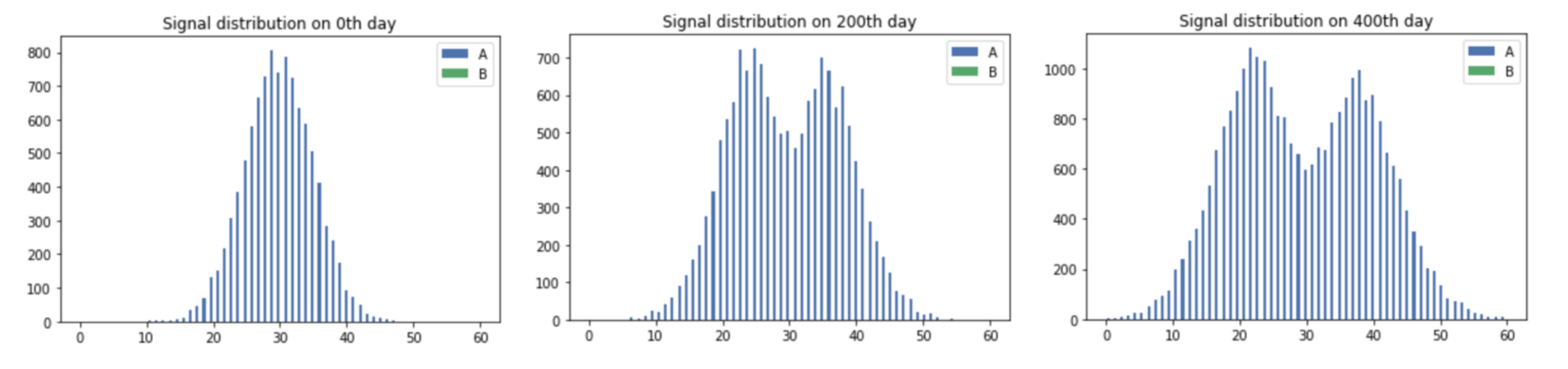
The predator preys on the signaling range with maximum utility. Thus signals that are produced by only the species with high utility will be the prime targets for the predator. On exploitation the prey species with high utility will naturally evolve to signaling range that is shared with a prey species of lower utility. The predator will learn that the common signaling range and associate it with the expected utility. Over generations, a drift in the signal is achieved (Figure  5).

Under the same notion, a prey species with low utility will drift away from prey species with higher utility. But this drift will be slower than the drift in case of a prey species with high utility.

This phenomena occurs when multiple prey species pool together which results in the predator not being able to distinguish between any of the species. This strategy results in an equilibrium as no species can be naturally selected and thus there is no induced drift.

Consider 3 prey species $A$,$B$, $C$ and predator $P$.
$A$ (Blue): constant high utility to $P$
$B$ (Green): constant low utility to $P$
$C$ (Red): constant medium utility to $P$

$u_{BP}(s)<u_{CP}(s)<u_{AP}(s)$

$\alpha_{B}=\alpha_{C}=\alpha_{A}$

As seen in Figure  6 the prey species enter a stable pooling equilibrium. This equilibrium is stable and persists because any change in the signal distribution of a single species will change the distribution of expected utility. This effectively will trigger a drift of all prey species such that the equilibrium is maintained.

This phenomena is the splitting of a single peaked signal distribution of a prey species to a multi-peak distribution. This dynamics can easily be seen in the case of non monotonic functions. Interestingly it is possible to generate the same phenomena using only simple linear monotonic functions.

We consider a situation where prey choose a trade-off between reproduction rate and toxicity. Higher toxicity implies a lower reproduction rate but also a lower utility to the predator.

Consider 3 prey species $A$, $B$, $C$ and predator $P$.
$A$ (Blue): Toxicity is high, utility to predator $P$ is low and reproduction rate is low
$B$ (Green):Toxicity is low, utility to predator $P$ is high and reproduction rate is high
$C$ (Red): Toxicity is moderate, utility to predator $P$ is moderate and reproduction rate is moderate

$u_{BP}(s)>u_{CP}(s)>u_{AP}(s)$

$\alpha_{B}<\alpha_{C}<\alpha_{A}$

In the scenario (Figure  7), prey species $B$ would have gone extinct. But instead we observe that in the presence of mimicry not only does prey species $B$ thrive at the end but also its signal splits into two peaks.

We show a situation where the mimicry of $A$ and $B$ results in mutual extinction. In the control ecosystem where the other does not exist, they actually thrive.

Consider 3 prey species $A$, $B$, $C$ and predator $P$.
$A$ (Blue): Utility to predator $P$ is negatively correlated to signal : $(u_{AP}(s)=a_{0}-a_{1}s)$
$B$ (Green): Utility to predator is constant and rate of mutation is insignificant : $(u_{BP}(s)=b_{0})$
$C$ (Red): Utility to predator is correlated to signal : $(u_{CP}(s)=c_{0}+c_{1}s)$

Since utility of $A$ is negatively correlated with signal it drifts towards the right ($R$) because the predator exploits $A$ of lower signal. Since utility of $C$ is correlated with signal it drifts towards the left ($L$) because the predator selects species $C$ of higher signal. Since, utility of $B$ is constant there is no drift but instead just a flattening of the signal distribution.

Oscillating mimicry where signals of two species is constantly oscillating, is not possible when we consider a one dimensional gene vector, identity signal function ($g$) and a fixed predator population. This situation is due to the formation of a pooling equilibrium.

Drift in higher dimensions is similar to 1-dimensional case except with more freedom.The drift is determined by the signal perception function, utility function of predator and genetic vector of prey.

Consider a prey species $A$ and a predator $P$. $A$ has a genetic constraint that it cannot reproduce if its genes are too different from the rest. This constraint stops the the signaling distribution from spreading out in all directions. The predator $P$ can see signals only along the line $s_{1}-s_{2}=k$ because of the signal perception function $f(s_{1},s_{2})=s_{1}+s_{2}$. Furthermore a utility function $u_{AP}(s_{1},s_{2})=s_{1}+s_{2}$ results in a diagonally left-down drift for the prey species $A$. The resulting drift of a 2-dimensional signal distribution has been illustrated in Figure  11

In the presence of two prey species and two predator species, we can create very interesting phenomena which involve changes in drift direction. Such directional change is not possible in 1-Dimensional signaling due to the creation of a Pooling Equilibrium.

Consider two prey species $A$, $B$ and two predator species $P$ and $Q$. Let the predators and prey have the following functions.

• •

  $P$ signal perception function : $f_{P}(s_{1},s_{2})=s_{1}$. This subcase means that $P$ can distinguish only the $x$ coordinate of the signal.

• •

  $Q$ signal perception function : $f_{Q}(s_{1},s_{2})=s_{2}$. This subcase means that $Q$ can only distinguish the $y$ coordinate of the signal.

• •

  The signaling function of $A$ as a function of the gene vector : $g_{A}(v_{1},v_{2})=(v_{2},-v_{1})$

• •

  The signaling function of $B$ as a function of the gene vector : $g_{B}(v_{1},v_{2})=(-v_{1},-v_{2})$

• •

  The utility function of $P$ as a function of gene vector : $u(v_{1},v_{2})\propto v_{1}+v_{2}$

• •

  The utility function of $Q$ as a function of gene vector : $u(v_{1},v_{2})\propto v_{1}-v_{2}$

The above functions result in the following utility functions.

• •

  $u_{AP}(s_{1},s_{2})\propto s_{1}-s_{2}$

• •

  $u_{AQ}(s_{1},s_{2})\propto-s_{1}-s_{2}$

• •

  $u_{BP}(s_{1},s_{2})\propto-s_{1}-s_{2}$

• •

  $u_{BQ}(s_{1},s_{2})\propto-s_{1}+s_{2}$

Starting at the appropriate positions with correct scaling parameters such that species $A$ has all the $x$ coordinates of its signal less then $B$ but $y$ coordinates of its signal greater than $B$. If initially $u_{AP}>u_{BP}$ and $u_{BQ}>u_{AQ}$, then $A$ will drift left but to predation by $P$ and $B$ will drift down due to predation by $Q$. The drift results in a mean x coordinate decrease for species A and a mean y coordinate decrease in signal for species B. As shown by the utility function the drift in species A results in decrease of $u_{AP}$ but an increase in $u_{AQ}$. Similarly, the drift in species B results in decrease of $u_{BQ}$ but an increase in $u_{BP}$. Thus after a point when $u_{AP}=u_{BP}$ and $u_{BQ}=u_{AQ}$, the predators start gaining interest in the other prey which they were not predating originally. Slowly the predators reduce the predating of their original prey and begin predating the other prey. This will result in $A$ drifting upward due to predation by $Q$ and $B$ drifting right due to predation by $P$.

So $A$ initially starts drifting left, followed by a gradual change in direction resulting in an upward drift. Similarly $B$ initially drifts downward and gradually shifts to drifting right.