Learning low bending and low distortion manifold embeddings © 2021 IEEE. Personal use of this material is permitted. Permission from IEEE must be obtained for all other uses, in any current or future media, including reprinting/republishing this material for advertising or promotional purposes, creating new collective works, for resale or redistribution to servers or lists, or reuse of any copyrighted component of this work in other works.

This paper investigates a loss functional for the geometric regularization of the latent manifold. Such a loss requires some geometric data of the input manifold in the training. We follow here a minimalistic approach involving data on distances and averages on the input manifold. We provide as testbed examples for which this data is explicitly known and easy to compute.

• •

  We propose to complement a discrete loss functional that promotes isometric embeddings in latent space with a discrete bending loss functional which prefers as flat as possible embeddings; this combination optionally permits to train the encoder on its own.
  

• •

  To train a corresponding autoencoder network we consider training data consisting of triplets of two input data points and their Fréchet average together with the distance between the two data points.
  

• •

  Unlike other isometry promoting approaches we do not approximate the Jacobian of the encoder (via backpropagation or complete correlation of all nearest neighbors) but use simple Monte Carlo point sampling.
  

• •

  Matching the theory of isometric maps, our numerical experiments confirm that the bending loss significantly increases smoothness of the resulting latent space manifold over a pure isometry loss. Also we find that the decoder maps linear interpolation in latent space to reasonable interpolations on the data manifold.
  

• •

  We demonstrate that our discrete loss functional is consistent with a well-posed, continuous limit functional on encoder maps from a smooth Riemannian data manifold into latent space.

The paper is structured as follows. Section 2 derives the new regularization loss and discusses its Monte Carlo limit for dense sampling of point pairs. The limit functional of this Monte Carlo limit for vanishing distance between the point pairs is introduced in section 3, and we prove existence of minimizers. As a proof of concept, we train autoencoders on three image datasets representing a priori known data manifolds. Section 4 describes the autoencoder set up, the experimental datasets, and the numerical results.

Denote the geodesic distance between two points $x,y\in M$ by $d_{M}(x,y)$ and their geodesic average by $\av_{M}(x,y)$. As input data to the training or optimization of the encoder $\phi$ we consider a sample $\mathcal{S}_{\epsilon}\subset\{(x,y)\in M\times M\,|\,d_{M}(x,y)\leq\epsilon\}$ of pairs $(x,y)\in M\times M$ of nearby points together with $d_{M}(x,y)$ and $\av_{M}(x,y)$. For a sufficiently small fixed locality radius $\epsilon>0$, the unique existence of the geodesic average is ensured. Our proposed loss function to regularize the encoder $\phi$ then reads

with first and second order difference quotients

where ${\gamma}(s)=|s|^{2}+|s|^{-2}-2$, $\av_{\mathbb{R}^{l}}(a,b)=(a+b)/2$ denotes the linear average in $\mathbb{R}^{l}$, and $\lambda>0$. Note that the first term in $E^{\mathcal{S}_{\epsilon}}$ has a strict minimum for $|\partial_{(x,y)}\phi|=1$. This term thus promotes $\lvert\phi(x)-\phi(y)\rvert=d_{M}(x,y)$ and thus low distortion and approximate isometry. The second term in $E^{\mathcal{S}_{\epsilon}}$ penalizes the deviation of intrinsic averages on $\phi(M)$ from extrinsic ones in $\mathbb{R}^{l}$. Note that this does not only penalize bending or any extrinsic curvature of $\phi(M)$ in $\mathbb{R}^{l}$, but in addition it also penalizes deviation of the inplane parameterization of $\phi(M)$ from a linear one (cf.the corresponding remark for $\Hess\phi$ in the next section). Examples of how to compute $\av_{M}$ and $d_{M}$ for image input data include the corresponding methods from the theories of LDDMM [You10], metamorphosis [TY05], or optimal transport [PC+19]. In our testbed we purposely used low-dimensional manifolds where $\av_{M}$ and $d_{M}$ are explicitly known.

Assuming that $\mathcal{S}_{\epsilon}$ is drawn uniformly from $M\times M$ (subject to the locality condition), our loss function $E^{\mathcal{S}_{\epsilon}}$ is up to $\mathcal{O}(\epsilon)$ the Monte Carlo integration of the energy

where $B_{\epsilon}^{M}(x)$ denotes the geodesic $\epsilon$-ball in $M$, centered at $x$, and where $\strokedint\ldots\mathrm{d}V_{g}$ denotes the mean with respect to the Riemann–Lebesgue volume measure on $M$ (the index $g$ indicates the Riemannian metric). As for the discrete functional $E^{\mathcal{S}_{\epsilon}}$, the energy $\mathcal{E}^{\epsilon}$ penalizes deviation from isometry and from intrinsically and extrinsically flat embeddings.

The energy $\mathcal{E}^{\epsilon}$ is rigid motion invariant by construction, i.e., composition of $\phi$ with a rigid motion does not change the energy. However, even apart from this invariance one cannot expect uniqueness of minimizers due to the nonconvexity of the first integrand. Whenever $M$ is intrinsically flat and homeomorphic to the $m$-disc (or at least globally compatible with an embedding into an $m$-dimensional Euclidean space), there is a unique minimizer of $\mathcal{E}^{\epsilon}$, though, as stated in the following proposition.

Note that this property of recovering flat embeddings may be quite relevant in applications as generative image manifolds were noticed in [SKTF18] to have almost no curvature.

In several applications one may already be content with a nice embedding $\phi$ that is specified only up to an affine transformation (rather than a rigid motion). Indeed, one may want to abandon isometry in favor of improving the approximation of geodesic averages by linear averages. This raises the question whether one can replace the integrand in (4) by some function $f(\partial_{(x,y)}\phi,\partial^{2}_{(x,y)}\phi)$ which is invariant under left composition of $\phi$ with invertible affine (and not just rigid) transformations. Yet, if $\partial_{(x,y)}\phi$ and $\partial^{2}_{(x,y)}\phi$ are non-parallel there is always an affine transform that maps $\partial_{(x,y)}\phi$ onto $(1,0,\cdots)$ and $\partial^{2}_{(x,y)}\phi$ onto $(0,1,0,\cdots)$ so that necessarily $f$ is of the form $f(a,b)\equiv c$ for $a$, $b$ non-parallel and $f(a,b)=h(s)$ for $b=sa$ with some constant $c$ and function $h:\mathbb{R}\to\mathbb{R}$. Thus, the regularizing properties would be lost. An alternative could be to just penalize $|\partial^{2}_{(x,y)}\phi|/|\partial_{(x,y)}\phi|$. Though not affinely invariant, it still encodes that geodesics should be close to linear interpolation without any competing isometry constraints ($|\partial_{(x,y)}\phi|$ in the denominator is needed for scale invariance and prevents a collapse to $\phi(M)=0$). Our loss $\mathcal{E}^{\epsilon}$ controls this flatness measure due to

Replacing $\mathcal{E}^{\epsilon}(\phi)$ with $\strokedint_{M}\strokedint_{B_{\epsilon}^{M}(x)}|\partial^{2}_{(x,y)}\phi|/|\partial_{(x,y)}\phi|\mathrm{d}y\,\mathrm{d}x$ would be infeasible, though: a straightforward calculation shows that a minimizing sequence of embeddings of the cylinder $M=S^{1}\times[0,1]$ into $\mathbb{R}^{l}$ would be cylinders of vanishing radius and diverging length.

The Riemannian gradient (Jacobian) $\Grad\phi(x)\in(T_{x}M)^{l}$ of $\phi$ is defined (denoting standard differentiation of smooth extensions onto $\mathbb{R}^{n}$ by $\grad$ ) via the identity

for all $v\in T_{x}M$, where $\exp_{x}:T_{x}M\to M$ denotes the Riemannian exponential map in $x$. An isometric embedding $\phi:M\to\mathbb{R}^{l}$ is characterized by $\Grad\phi(x)$ being orthogonal in any point $x\in M$. Thus, deviation from an isometric embedding manifests as non-unit singular values of $\Grad\phi(x)$. Similarly, extrinsic bending of the embedding $\phi(M)$ manifests as a non-vanishing Riemannian Hessian $\Hess\phi$ of $\phi$, where the Riemannian Hessian at $x$ is the linear operator

for $\nabla$ the Levi-Civita connection and $\nabla_{v}$ the covariant derivative in direction $v$ [AMS09, Chp. 5]. The associated quadratic form $\hess\phi(x):T_{x}M\times T_{x}M\to\mathbb{R}^{l}$ is

where the Riemannian metric $g$ on $(T_{x}M)^{l}\times T_{x}M$ is applied componentwise, i.e., we use the notation $g(A,v)=(g(A_{j},v))_{j=1,\ldots,l}$ for a matrix whose rows $A_{j}$ are tangent vectors. A natural loss function to promote low distortion and low bending embeddings thus reads

where $\|A\|_{F}^{2}=\tr(A^{*}A)$ is the Frobenius norm of an operator $A$ and $B\mapsto{\Gamma}(B)$ is an admissible function, i.e., a nonnegative function depending only on the singular values of $B$ and being zero if and only if all of them are one.

Let us remark that the orthogonal projection of $\Hess\phi(x)$ onto the normal bundle $[T_{\phi(x)}\phi(M)]^{\perp}$ of $\phi(M)$ is the second fundamental form of $\phi(M)$ pulled back onto $T_{x}M$. If $m=2$ and $l=3$, this is also known as the Weingarten map or shape operator relative to $T_{x}M$. In addition to penalizing this second fundamental form, which indicates extrinsic bending of $\phi(M)$, our functional $\mathcal{E}$ also penalizes the tangential components of $\Hess\phi$.

The above energy can be rewritten in terms of averages. To this end, let $S^{m-1}$ denote the unit sphere in $T_{x}M$ (the base point $x$ will be clear from the context), and let $\mathcal{H}^{m-1}$ denote the $(m-1)$-dimensional Hausdorff measure in $T_{x}M$.

It turns out that for $\epsilon\to 0$ our loss $\mathcal{E}^{\epsilon}$ approximates $\mathcal{E}$, which thus gives a simple interpretation of $\mathcal{E}^{\epsilon}$ in terms of first and second order derivatives of $\phi$.

Let us now establish the existence of minimizers to $\mathcal{E}$. First, we observe that the energy $\mathcal{E}$ is well-defined on all of $H^{2}(M)$, where the Sobolev space $H^{2}(M)$ is defined as the closure of all smooth functions under the norm $\|\phi\|_{H^{2}(M)}$ with

For further details on Sobolev spaces on (compact) manifolds we refer to [Heb96]. Due to the rigid motion invariance of $\mathcal{E}$ we may without loss of generality restrict $\mathcal{E}$ to the subspace $\dot{H}^{2}(M)$ of $H^{2}$-functions with zero average.

If $l\geq 2m$ the condition is always fulfilled since by Whitney’s embedding theorem there exists a smooth embedding which, due to the compactness of $M$, may be chosen such that it has finite energy.

Just as for $\mathcal{E}^{\epsilon}$, the minimizer (modulo a rigid motion) is in general not unique due to the isometry promoting term.

We consider an image resolution of $64\times 64$. The images are generated as follows.

(G) Anisotropic Gaussians. We consider rotations, scalings, and translations of a cut off Gaussian of fixed aspect ratio, with parameters $(\alpha,s,x)\in M=S^{1}\times[a,b]\times[c,d]^{2}$ with distance

where $d_{S^{1}}$ is the geodesic distance on $S^{1}$. The data is similar to the DSprites dataset in [MHHL17].

(S) Sundials. Inspired by [OYHO20], we generate images parametrized by the upper hemisphere $M=S^{2}\cap\{x_{3}\geq 0\}$ by casting a shadow of a vertical rod on a plane. Contrary to [OYHO20] we do not render these images with a 3D engine, but instead simply approximate the shadows by Gaussians (cf.fig. 1): a point $x\in M$ is first mapped onto the plane by drawing the line through $x$ and the rod tip, intersecting the plane at some $y\in\mathbb{R}^{2}$. We then use a Gaussian function with variance $\lvert y\rvert$ in direction $y$ and a fixed small variance in the orthogonal direction, centered at $y/2$. As distance on $M$ we use the geodesic distance on $S^{2}$, $d(x,x^{\prime})=\arccos(x^{T}x^{\prime})$.

(R) Rotated 3D objects. We generate images by rotating a camera pointing at a three-dimensional object, Spot the cow¹¹ 1 https://www.cs.cmu.edu/ kmcrane/Projects/ModelRepository/. We use Pytorch3D [RRN+20] to render the images during training. As distance on $M=SO(3)$ we use the geodesic distance computed via quaternions as $d(q_{1},q_{2})=\arccos(\lvert q_{1}\cdot q_{2}\rvert)$ [Huy09].

The used architecture is as in [BRRG18], however, we used larger input images and a smaller latent dimensionality. The encoder consists of a first layer of $1\times 1$ convolutions with $16$ output channels, followed by blocks consisting of two consecutive $3\times 3$ convolutions with unit stride, zero padded such that the input and output width are equal, and $2\times 2$ average pooling. Each of the convolutional layers in the block is followed by a leaky ReLU nonlinearity with slope $-0.01$. The first convolution in each block doubles the output channels. The final convolution is not followed by a nonlinearity and has only 1 (4 for (R)) output channel(s). The number of convolutional blocks determines the size of the latent code: we used $4$ blocks with input images of size $64\times 64$ ($64\times 64\times 3$ for (R)), resulting in a latent code of size $16$ ($64$ for (R)). The decoder also consists of consecutive blocks of two $3\times 3$ convolutions with leaky ReLU nonlinearities, where each block is followed by $2\times 2$ nearest neighbor upsampling. The final convolutional layer is again not followed by a nonlinearity and has 1 output channel. We use Kaiming initialization [HZRS15], i.e., all convolutional weights are initialized as zero-mean Gaussian random variables with standard deviation $\sqrt{2}/\sqrt{\texttt{fan\char 95\relax in}(1+0.01^{2})}$ for fan_in the layer input dimension, and all biases are initialized with zeros. For training, we use the Adam optimizer [KB15] with learning rate $0.0001$ and default values for $\beta_{1},\beta_{2}$ and $\varepsilon$. The training data are triplets of images plus a distance value (cf.fig. 1 top),

with $x,y\in\mathcal{S}_{\epsilon}\subset M$, $\av_{M}(x,y)$ the geodesic average of $x,y$ in $M$ and $d_{M}(x,y)$ their geodesic distance. This input allows to compute the ingredients $\partial_{(x,y)}\phi$ and $\partial^{2}_{(x,y)}\phi$ of the loss functional $E^{\mathcal{S}_{\epsilon}}(\phi)$ defined in section 2.

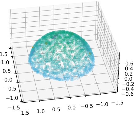
Figure 1 summarizes our approach and its result at one glance for dataset (S); the top box shows examples of training triplets plus distances, the middle box visualizes the obtained manifold embedding $\phi(M)$, and the bottom box displays reconstructions of input images by the full autoencoder.

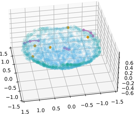Figures 2, 5 and 6 show further obtained manifold embeddings in latent space for different loss weights and for the datasets (R) and (G). In all cases we observe smooth embeddings that neatly reproduce the geometry and topology of the underlying manifold $M$. For visualizing the manifold embeddings $\phi(M)$ we simply perform a principal component analysis (PCA) in latent space and display the resulting top three dimensions (in fig. 5 a second set of principal components is shown in addition). To illustrate that our approach allows separate training of encoder and decoder, for fig. 1 we first trained the encoder map $\phi$ on its own by minimizing $E^{\mathcal{S}_{\epsilon}}(\phi)$ and subsequently trained the decoder map $\psi$ by minimizing, for fixed $\phi$, the reconstruction loss

with $\|\cdot\|_{L^{2}}$ the $L^{2}$-norm on images. For the other datasets we train en- and decoder simultaneously by jointly minimizing $E^{\mathcal{S}_{\epsilon}}(\phi)+\kappa R(\phi,\psi)$ for $\phi$ and $\psi$ (where the weight $\kappa>0$ is not expected to have much influence since $\psi$ will try to minimize $R(\phi,\psi)$ anyhow). We use $\epsilon=\frac{\pi}{2}$ for dataset (S), $\epsilon=\frac{\pi}{4}$ for (R). For (G), for simplicity we used a slightly different sample $\hat{\mathcal{S}}_{\epsilon}\subset\{(y,y^{\prime})\in M\times M\,|\,d_{S^{1}}(\alpha,\alpha^{\prime})\leq\epsilon\}$ with $\epsilon=\frac{\pi}{2}$. During training the isometry, flatness, and reconstruction parts of the loss function are all observed to decrease continuously and monotonically (up to the usual stochastic variations) as shown in fig. 3 for dataset (R), where the full autoencoder is trained simultaneously. Resulting reconstructions $\psi(\phi(x))$ for random $x\in M$ are exemplarily shown in figs. 1 and 6 and are of good quality. Figure 2 illustrates the effect of the flatness term: for zero bending penalization $\lambda$ one obtains a standard isometric embedding of $S^{2}$, while it gets flattened for higher values of $\lambda$ (fig. 1 shows an intermediate $\lambda$). Note that extrinsic bending is obviously reduced this way, while nonlinear inplane distortion is increased (the normal component of the Hessian apparently outweighs the inplane component).

Figure 5 illustrates for dataset (R) that the bending term of our loss functional strongly improves the usefulness of linear interpolation in latent space across moderate distances. While for $\lambda=0$ the decoder output of linear interpolations in latent space does not at all reproduce continuously rotating objects, it clearly does for bending weight $\lambda=10$. Let us emphasize that the decoder was in no way regularized in these experiments, in particular it was not trained on any points obtained via linear interpolation of codes in latent space! Still the rotated cow is cleanly visible (in contrast to the case $\lambda=0$), having undergone merely some minor smoothing. Training the decoder additionally on linear interpolants in latent space will naturally improve the results. We purposely abstained from this extra regularization since it would allow the decoder to compensate the deficiencies visible for $\lambda=0$ so that the regularizing properties of our encoder loss functional $E^{\mathcal{S}_{\epsilon}}$ would be obscured. For $\lambda=10$ the decoder has to compensate much less and is therefore expected to be more robustly trainable. We also quantitatively evaluated the quality of linear interpolation in latent space by measuring the $L^{2}$-error to the ground truth, geodesic interpolation. We calculate this on a test sample set $\mathcal{S}_{\epsilon}^{\prime}$ as

where $\av_{M}(x,y;t)$ is the weighted geodesic average of $x,y\in M$ with weights $1-t,t$ and $\av_{\mathbb{R}^{l}}(a,b;t)=(1-t)a+tb$. Above, $\mathrm{err}_{\text{i}}$ is the error due to linear interpolation, and $\mathrm{err}_{\text{b}}$ is the base reconstruction error which occurs independently of interpolation. Figure 4 displays $\mathrm{err}(t)$ for different values of $\lambda$, showing a marked error reduction for increasing $\lambda$ up to a saturation around $\lambda=5$.

In our experiments, we set the latent space dimensionality $l$ to commonly used values. In particular, we take $l$ substantially larger than would minimally be required for a smooth embedding. This is reasonable since in applications the intrinsic dimensionality $m$ is generally unknown and since this allows the encoder to improve on the flatness of the embedding at the expense of using more dimensions. For example, the flat torus should better be embedded as $S^{1}\times S^{1}\subset\mathbb{R}^{4}$ than as a torus in $\mathbb{R}^{3}$. Figure 5 shows that the encoder makes use of that freedom: even though $l=5$ would be enough ($SO(3)\cong\mathbb{R}P^{3}$, which embeds into $\mathbb{R}^{5}$, but not $\mathbb{R}^{4}$ [Hop40, Han38]), the graph of the standard variation along the principal components of latent space shows that 9 Euclidean dimensions are used for the embedding. For the experiments with datasets (S) and (G), the embedding used 3 and 5 Euclidean dimensions, respectively.

To illustrate the regularization properties of our loss functional we avoided sources of noise in our experiments, as those would require additional tailored regularization. For the anisotropic Gaussian (G) we now illustrate what effect a simple type of noise can have on the embedding $\phi$ without additional regularization: we simply round all Gaussian images to binary images. This quantization makes ellipses in nearby positions, orientations and scalings harder to distinguish. Figure 6 right shows that a cylindrical structure of the resulting latent manifold $\phi(M)$ is still observable, though it is thickened and much less clean than on the left.

This work was supported by the Deutsche Forschungsgemeinschaft (DFG, German Research Foundation) via project 211504053 - Collaborative Research Center 1060 and via Germany’s Excellence Strategy project 390685813 - Hausdorff Center for Mathematics and project 390685587 - Mathematics Münster: Dynamics-Geometry-Structure.

References

- [ABP19] Andrei A. Agrachev, Davide Barilari, and Elisa Paoli. Volume geodesic distortion and Ricci curvature for Hamiltonian dynamics. Annales de l’Institut Fourier, 69(3):1187–1228, 2019.
- [AGL20] Matan Atzmon, Amos Gropp, and Yaron Lipman. Isometric autoencoders. arXiv preprint arXiv:2006.09289, 2020.
- [AMS09] P-A Absil, Robert Mahony, and Rodolphe Sepulchre. Optimization algorithms on matrix manifolds. Princeton University Press, 2009.
- [BRRG18] David Berthelot, Colin Raffel, Aurko Roy, and Ian Goodfellow. Understanding and improving interpolation in autoencoders via an adversarial regularizer. arXiv preprint arXiv:1807.07543, 2018.
- [DG03] David L Donoho and Carrie Grimes. Hessian eigenmaps: Locally linear embedding techniques for high-dimensional data. Proceedings of the National Academy of Sciences, 100(10):5591–5596, 2003.
- [DG05] David L Donoho and Carrie Grimes. Image manifolds which are isometric to Euclidean space. Journal of mathematical imaging and vision, 23(1):5–24, 2005.
- [Han38] W. Hantzsche. Einlagerung von Mannigfaltigkeiten in euklidische Räume. Math. Z., 43(1):38–58, 1938.
- [Heb96] Emmanuel Hebey. Sobolev spaces on Riemannian manifolds, volume 1635. Springer Science & Business Media, 1996.
- [Hop40] Heinz Hopf. Systeme symmetrischer Bilinearformen und euklidische Modelle der projektiven Räume. Vierteljschr. Naturforsch. Ges. Zürich, 85(Beiblatt (Festschrift Rudolf Fueter)):165–177, 1940.
- [Huy09] Du Q. Huynh. Metrics for 3d rotations: Comparison and analysis. J. Math. Imaging Vis., 35(2):155–164, October 2009.
- [HZRS15] Kaiming He, Xiangyu Zhang, Shaoqing Ren, and Jian Sun. Delving deep into rectifiers: Surpassing human-level performance on imagenet classification. In Proceedings of the IEEE International Conference on Computer Vision (ICCV), December 2015.
- [KB15] Diederik P. Kingma and Jimmy Ba. Adam: A method for stochastic optimization. In Yoshua Bengio and Yann LeCun, editors, 3rd International Conference on Learning Representations, ICLR 2015, San Diego, CA, USA, May 7-9, 2015, Conference Track Proceedings, 2015.
- [KZSN20] Keizo Kato, Jing Zhou, Tomotake Sasaki, and Akira Nakagawa. Rate-distortion optimization guided autoencoder for isometric embedding in Euclidean latent space. In International Conference on Machine Learning, pages 5166–5176. PMLR, 2020.
- [MF11] Yunqian Ma and Yun Fu. Manifold learning theory and applications. CRC press, 2011.
- [MHHL17] Loic Matthey, Irina Higgins, Demis Hassabis, and Alexander Lerchner. dsprites: Disentanglement testing sprites dataset. https://github.com/deepmind/dsprites-dataset/, 2017.
- [OYHO20] Alon Oring, Zohar Yakhini, and Yacov Hel-Or. Autoencoder image interpolation by shaping the latent space, 2020.
- [PC+19] Gabriel Peyré, Marco Cuturi, et al. Computational optimal transport: With applications to data science. Foundations and Trends® in Machine Learning, 11(5-6):355–607, 2019.
- [PLD+20] Erez Peterfreund, Ofir Lindenbaum, Felix Dietrich, Tom Bertalan, Matan Gavish, Ioannis G Kevrekidis, and Ronald R Coifman. Local conformal autoencoder for standardized data coordinates. Proceedings of the National Academy of Sciences, 117(49):30918–30927, 2020.
- [PTBK19] Gautam Pai, Ronen Talmon, Alex Bronstein, and Ron Kimmel. Dimal: Deep isometric manifold learning using sparse geodesic sampling. In 2019 IEEE Winter Conference on Applications of Computer Vision (WACV), pages 819–828. IEEE, 2019.
- [RPC+07] Marc Ranzato, Christopher Poultney, Sumit Chopra, Yann LeCun, et al. Efficient learning of sparse representations with an energy-based model. Advances in neural information processing systems, 19:1137, 2007.
- [RRN+20] Nikhila Ravi, Jeremy Reizenstein, David Novotny, Taylor Gordon, Wan-Yen Lo, Justin Johnson, and Georgia Gkioxari. Accelerating 3d deep learning with pytorch3d. arXiv:2007.08501, 2020.
- [RS00] Sam T Roweis and Lawrence K Saul. Nonlinear dimensionality reduction by locally linear embedding. science, 290(5500):2323–2326, 2000.
- [RVM+11] Salah Rifai, Pascal Vincent, Xavier Muller, Xavier Glorot, and Yoshua Bengio. Contractive auto-encoders: Explicit invariance during feature extraction. In Icml, 2011.
- [SKTF18] Hang Shao, Abhishek Kumar, and P Thomas Fletcher. The Riemannian geometry of deep generative models. In Proceedings of the IEEE Conference on Computer Vision and Pattern Recognition Workshops, pages 315–323, 2018.
- [ST19] Ariel Schwartz and Ronen Talmon. Intrinsic isometric manifold learning with application to localization. SIAM Journal on Imaging Sciences, 12(3):1347–1391, 2019.
- [TDSL00] Joshua B Tenenbaum, Vin De Silva, and John C Langford. A global geometric framework for nonlinear dimensionality reduction. science, 290(5500):2319–2323, 2000.
- [TY05] Alain Trouvé and Laurent Younes. Local geometry of deformable templates. SIAM J. Math. Anal., 37(1):17–59, 2005.
- [VLBM08] Pascal Vincent, Hugo Larochelle, Yoshua Bengio, and Pierre-Antoine Manzagol. Extracting and composing robust features with denoising autoencoders. In Proceedings of the 25th international conference on Machine learning, pages 1096–1103, 2008.
- [You10] Laurent Younes. Shapes and diffeomorphisms, volume 171 of Applied Mathematical Sciences. Springer-Verlag, Berlin, 2010.