Efficient channel charting via phase-insensitive
distance computation
Abstract
Channel charting is an unsupervised learning task whose objective is to encode channels so that the obtained representation reflects the relative spatial locations of the corresponding users. It has many potential applications, ranging from user scheduling to proactive handover. In this paper, a channel charting method is proposed, based on a distance measure specifically designed to reduce the effect of small scale fading, which is an irrelevant phenomenon with respect to the channel charting task. A nonlinear dimensionality reduction technique aimed at preserving local distances (Isomap) is then applied to actually get the channel representation. The approach is empirically validated on realistic synthetic multipath MIMO channels, achieving better results than previously proposed approaches, at a lower cost.
Index Terms:
channel charting, dimensionality reduction, MIMO signal processing, machine learning.I Introduction
Machine learning techniques have been applied with success to several wireless communication problems in recent years [1]. However, most of these techniques fall within the supervised learning paradigm, and thus require labeled data to operate. The acquisition of such data may be unpractical or complex to implement within existing communication systems.
Channel charting [2] on the other hand is a fully unsupervised learning task. Indeed, its objective is for a multi-antenna base station to build a low-dimensional map (called chart) of the radio environment based on uplink channel measurements, without requiring access of the users’ actual locations. The chart should reflect as much as possible the physical reality, in the sense that the charting function should preserve spatial neighborhoods. Predicting this way the relative locations of users from channel measurements has many potential applications, ranging from SNR prediction [3] and pilot reuse [4], to user grouping, proactive handover management or beam-finding (see [2] for more details on potential applications). What makes channel charting particularly interesting compared to classical positioning methods is its fully unsupervised nature. Indeed, no link with the application layer in order to get locations from a global navigation satellite system (GNSS) is required (even offline to build a dataset). Only channel measurements are needed, which are readily accessible from the radio access network (RAN). Moreover, having access to the relative locations of users instead of their absolute locations is sufficient for most applications that need to assess the proximity of users. In that sense channel charting can be seen as an unsupervised alternative to radio maps [5].
Contributions. This paper proposes a computationally efficient method to perform channel charting, based on the computation of a distance measure that is designed to be insensitive to small scale fading and to locally reflect physical distance. This measure is theoretically motivated based on a simple physical channel model. It allows to compute a distance matrix from the training channels, which is then used within the Isomap [6] nonlinear dimensionality reduction method to get the chart coordinates. The proposed method is empirically assessed on channel data used in [2], for which it yields better results than previously proposed approaches at a lower computational cost. The method is also assessed on higher-dimensional channels for which some of the previously proposed methods are too costly to be applied.
Related work. In the seminal paper on channel charting [2], the raw second order moment of channels is used as input features in order to reduce the influence of small scale fading which is irrelevant to the channel charting task. Such features have the disadvantage of being of dimension equal to the square of the channel dimension. On the other hand, it was more recently proposed to use the channel autocorrelation as input features [7]. This has the advantage of yielding features of the same dimension as the channel that are also quite insensitive to small scale fading. However, using autocorrelations automatically makes the features translation invariant in the angular and delay domains, which is a potentially harmful property with respect to the channel charting task, especially for channels in line of sight (LoS) or comprising a dominant path. In contrast, the method proposed in this paper does not require to square the channel dimension nor introduces any invariance in the angular or delay domain. Finally, it is interesting to notice that the distance measure used in this paper was also used for supervised learning tasks such as user positioning and channel mapping in a previous work [8], although it was not theoretically motivated.
II Problem formulation
The method proposed in this paper applies to a wide variety of multi-user massive multiple input multiple output (massive MIMO) wideband systems [9, 10], operating indifferently in time division duplex (TDD) or frequency division duplex (FDD), where the antennas at the base station are indifferently colocated or not (in which case it is a distributed MIMO system). Let us consider base station antennas and subcarriers evenly distributed at frequencies around a center frequency spanning a total bandwidth , and denote the uplink channel vector between any given user and the base station and the channel for the th antenna on the th subcarrier. In order to lighten notations, the total channel dimension is denoted . Note that no index is introduced to denote to which specific user corresponds the channel, since the proposed method treats indifferently the channels from all users.
Based on a database of estimated uplink channels
| (1) |
the objective in this paper is to build a forward charting function (or simply charting function)
| (2) |
where is the vector in the chart associated to channel and is the chart dimension. Note that, as opposed to [2], no feature extraction step is considered, so that the forward charting function directly operates on estimated channels.
Performance measures. In order to evaluate charting functions, the location of the user yielding channel is denoted , where is the number of considered spatial dimensions (two or three). A charting function is considered good if it preserves neighborhoods. Mathematically, it corresponds to the property
| (3) |
being true for any using the Euclidean distance. In order to quantify this rather vague requirement, and following [2], the performance measures used in this paper are the continuity (CT) and trustworthiness (TW), which are classical performance measures for dimensionality reduction methods [11]. Both measures are between zero and one (the higher the better). Continuity assesses whether channels corresponding to nearby locations are mapped to nearby vectors in the chart (forward implication in (3)). Its precise expression is
| (4) |
where corresponds to the rank (in terms of proximity measured with the Euclidean distance) of the charted channel with respect to ( if is the -th closest to considering all the charted channels), and is the set containing indices of channels being among the closest to the th in space but not in the chart. if the nearest neighbors of all considered channels in terms of spatial location are all mapped among the nearest neighbors of their representation on the chart, then . On the contrary, if the nearest neighbors of all considered channels in terms of spatial location are all mapped among the furthest of their representation on the chart, then . On the other hand, trustworthiness assesses whether nearby vectors in the chart do correspond to spatially close users (converse implication in (3)). It is defined in a very similar way as continuity, except that the roles of the spatial locations and locations on the chart are switched. It is expressed as
| (5) |
where corresponds to the rank (in terms of proximity measured with the Euclidean distance) of the location with respect to , and is the set containing indices of channels being among the closest to the th in the chart domain but not in space.
III Forward charting function
In this section, the proposed forward charting function is introduced and explained in details. The general strategy is to first design a distance measure between channels that preserves spatial neighborhoods and then use it to compute chart coordinates via a nonlinear dimensionality reduction method.
III-A Distance measure
In order to set up the proposed method, a distance measure between channels which locally reflects physical reality (locations of the corresponding users) is first sought. If the Euclidean distance between channel vectors preserved spatial neighborhoods, no charting would be needed. However, this is not the case for several reasons. First of all, as noticed in [2, Figure 4], using as distance measure
| (6) |
makes channels corresponding to users far away from the base station appear closer to one another and channels corresponding to users close to the base station appear further away to one another. This issue can be partly resolved by normalizing channels (for example simply dividing channel vectors by their -norm [7]), using the distance
| (7) |
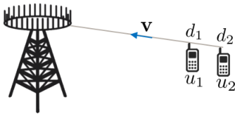
However, the Euclidean distance between normalized channels given in (7) is still unsatisfactory. This can be seen with a very simple example exposing a pathological situation. Imagine two users and located in the same direction with respect to the base station at distance and (as shown on figure 1). Using the plane wave assumption, and considering a single propagation path, the normalized channels of users and can both be expressed as
| (8) |
where is the wavelength (at the central frequency), is the time delay, is the steering vector associated with direction (see [12, 13] for their complete definitions) and is the vector of relative phase differences along subcarriers associated to delay (simply equivalent to a steering vector in the frequency domain). Now, if the two users are separated by half a wavelength, assuming that the bandwidth is much smaller than the central frequency (), the two normalized channels are almost opposite vectors:
| (9) |
This is because in that case, and . In other words, normalized channels are almost maximally far away while users are very close (a few centimeters at usual carrier frequencies). This simple example shows that the Euclidean distance between channels is very sensitive to small scale fading, which is clearly a harmful behavior with respect to the channel charting task. This sensitivity comes from the very fast changes in the global phase of channels due to small movements of users. In order to overcome this issue, a distance measure which is totally insensitive to the global phase of channels is proposed here:
| (10) |
In the context of the previous example, this distance measure yields for and a monotonically increasing value of with (for values of up to several meters for classical systems). This distance measure allows to get rid of the oscillating behavior (of period ) of the distance given in (7) with respect to which is due to small scale fading. The distance may seem difficult to compute at first sight, because of the involved optimization problem. However, it can be expressed simply as
| (11) |
The proof of this equality is given in appendix A. It means that taking the modulus of the inner product (instead of the real part) implicitly corresponds to put channels in phase (without needing to solve an optimization problem). Under this form, is easy to compute. Note that the distance measure is introduced here motivated by a simple example, but it is illustrated on realistic channels (comprising several paths) in the experimental section.
Compared to previously proposed channel charting methods, using this phase-insensitive distance allows to gain insensitivity to small scale fading without introducing features of dimension (as proposed in [2]), nor having to lose all sensitivity to absolute direction and delay (as is the case when using autocorrelations as input features [7]).
III-B Chart coordinates
Now that a distance measure has been chosen, the chart coordinates remain to be obtained. The objective is to find a global coordinate system in dimensions (with ) in which the Euclidean distances between training samples are as close as possible to the distances measured with (that should be close to the spatial distance between users). To do so, a dimensionality reduction method can be applied.
It is interesting to notice that distances measured with reflect physical distances only locally (only small values of are reliable). Indeed, a small value for corresponds to nearby users, but a large value for does not necessarily correspond to far away users. In such a situation, the Isomap method [6] is particularly adapted. Indeed, it is based on the assumption that it is possible to reliably compute small distances between training samples but not large ones. It is based on a neighborhood graph (considering neighbors), from which large distances are estimated by finding shortest paths. In the studied context, this allows to approximate large distances using only small values of . Then, multidimensional scaling (MDS) [14] is applied to the obtained distance matrix to get a low dimensional embedding (see [6, 15] for a detailed description of Isomap). In the sequel, denotes the matrix whose columns are the result of the Isomap method applied to the input distance matrix with an embedding in dimensions considering the nearest neighbors to build the neighborhood graph. In practice, the scikit-learn [16] implementation of Isomap is used. The proposed method is summarized in algorithm 1.
Computational complexity. One of the main advantages of the proposed method compared to prior art is its low complexity with respect to the channel dimension and number of training channels . Indeed, the distance computation step has complexity , while the dimensionality reduction step has complexity [17, 16]. Note that the original channel charting methods based on raw second order moments [2] have complexity at least , or require to train a neural network (whose complexity is difficult to precisely quantify but which takes time in practice).
In summary, the proposed method is particularly adapted to high-dimensional channels (large ), with relatively few examples (not too large ). However, if a lot of examples are available, one can perfectly envision to use landmark Isomap [18] instead of the classical Isomap. This would allow to reduce complexity of the method to for the first step and for the second, with being the number of considered landmarks.
IV Experiments
In this section, the proposed method is empirically assessed on several kinds of MIMO channels. At first, and in order to compare to previously proposed methods [2, 19], training channels obtained with the Quadriga channel simulator [20] are used. Then, higher dimensional channels taken from the DeepMIMO dataset [21] are considered. In all the following experiments, the dimension of the chart is fixed to . Besides the obvious advantage of this choice for visualizing the chart, it comes from the fact that if users are distributed on a 2D-plane, then the channel manifold should be two-dimensional (see [8, Section III.C] for a more detailed explanation of this point). One could of course optimize the chart dimension empirically. This option is left to future work.
IV-A Quadriga channels
For this first set of experiments, exactly the same multipath channels as those used in [2] are considered. Namely, users are randomly located in an area of and their channels are obtained considering an urban macrocell environment at a center frequency of within the Quadriga channel simulator [20] (details available in [2, Table I]). User locations are shown on figure 2, the base station being at the origin and equipped with an uniform linear array (ULA) of half-wavelength separated antennas. The dimension of these training channels is , and they are assumed to be acquired at an SNR of and averaged over time instants.
Results. The obtained chart for and is shown on figure 3 (in the nLoS case). Neighborhoods are quite well preserved, although channels seem to be mapped on a circle. This may be explained by the fact that using a single subcarrier makes the system insensitive to delay, so that only angle discrimination is possible (no distance information appears on the chart). Results in terms of continuity (CT) and trustworthiness (TW) are shown on the leftmost (LoS) and center (nLoS) parts of figure 6, where it is compared to the original channel charting methods of [2] (PCA, SM, SM+ and AE, see [2] for the details of each method). The obtained performance is very good. Indeed, the proposed method outperforms previously proposed methods in terms of continuity and is at the same level in terms of trustworthiness, while being more computationally efficient. Indeed, it does not require to compute high dimensional features, which is the case for the concurrent methods which use raw second order moments of dimension . The proposed method runs in less than seconds on a regular laptop (Intel(R) Core(TM) i5-6300U CPU @ 2.40 GHz), which makes it very fast. Moreover, note that the proposed method is also better than the previously proposed method that uses channel autocorrelation as input features (see [19, Table II], “Plain” column to precisely compare).
IV-B DeepMIMO channels
For this second experiment, training multipath channels are taken from the DeepMIMO dataset [21]. The ‘O1’ urban outdoor ray-tracing scenario is chosen (with paths per channel), with a single base station (BS ) and a subset of all possible user locations. The scenario is depicted on figure 4, where the colorized points correspond to users whose channels are in the training data, and the base station is circled in red. The base station is equipped with a square uniform planar array (UPA) with half-wavelength separated antennas at a central frequency of , with subcarriers evenly spaced spanning a band of . This results in channels of dimension . No noise is added for this experiment. Note that, as opposed to the previous experiment, only a single time instant is considered here for the channels (no averaging is done).

Results. The obtained chart for and is shown on figure 5, where it is seen that spatial neighborhoods are well preserved. In particular, thanks to the fact that several subcarriers are considered (as opposed to the previous experiment), the system exhibits sensitivity to delay, so that both the angle and distance information are expressed in the chart. Regarding the CT and TW performance measures for a varying number of neighbors , results are shown on the rightmost part of figure 6. The performance seems better than for the Quadriga channels, which may be explained by the fact that channels are noiseless. More interestingly, the proposed charting method runs in less than seconds on a regular laptop, even though channels are high-dimensional (). This is promising for its applicability, since concurrent methods [2, 19] would take much more time for such channels. For example, the raw second order moment for such channels would comprise entries, this is why methods of [2] are not compared to the proposed one for these channels.


V Conclusion and perspectives
In this paper, a computationally efficient channel charting method was introduced. It is based on the computation of a distance measure between channel vectors which is designed to be insensitive to small scale fading. The distance matrix obtained with this measure is then used within the Isomap nonlinear dimensionality reduction method in order to obtain the chart coordinates. The proposed method is assessed on realistic multipath channels of various dimensions, showing great potential in terms of accuracy and computational efficiency.
In the future, several research leads could be investigated in the continuation of this paper. First of all, it would be interesting to handle out of sample channels in order to allow for online implementations in practical systems. Second, the method could be used as an initialization for a deep neural network in order to perform fine tuning (as done for example in [8] for channel mapping and user positioning).
Appendix A Proof of equation (11)
The proof starts with a re-expression of the norm as
Then, using and noticing that for concludes the proof.
References
- [1] T. O’Shea and J. Hoydis, “An introduction to deep learning for the physical layer,” IEEE Transactions on Cognitive Communications and Networking, vol. 3, no. 4, pp. 563–575, 2017.
- [2] C. Studer, S. Medjkouh, E. Gönültaş, T. Goldstein, and O. Tirkkonen, “Channel charting: Locating users within the radio environment using channel state information,” IEEE Access, vol. 6, pp. 47 682–47 698, 2018.
- [3] P. Kazemi, H. Al-Tous, C. Studer, and O. Tirkkonen, “Snr prediction in cellular systems based on channel charting,” in 2020 IEEE Eighth International Conference on Communications and Networking (ComNet), 2020, pp. 1–8.
- [4] L. Ribeiro, M. Leinonen, H. Djelouat, and M. Juntti, “Channel charting for pilot reuse in mmtc with spatially correlated mimo channels,” in 2020 IEEE Globecom Workshops (GC Wkshps, 2020, pp. 1–6.
- [5] S. Bi, J. Lyu, Z. Ding, and R. Zhang, “Engineering radio maps for wireless resource management,” IEEE Wireless Communications, vol. 26, no. 2, pp. 133–141, 2019.
- [6] J. B. Tenenbaum, V. De Silva, and J. C. Langford, “A global geometric framework for nonlinear dimensionality reduction,” science, vol. 290, no. 5500, pp. 2319–2323, 2000.
- [7] E. Gönültaş, E. Lei, J. Langerman, H. Huang, and C. Studer, “Csi-based multi-antenna and multi-point indoor positioning using probability fusion,” 2020.
- [8] L. Le Magoarou, “Similarity-based prediction for channel mapping and user positioning,” IEEE Communications Letters, pp. 1–1, 2021.
- [9] F. Rusek, D. Persson, B. K. Lau, E. G. Larsson, T. L. Marzetta, O. Edfors, and F. Tufvesson, “Scaling up mimo: Opportunities and challenges with very large arrays,” IEEE Signal Processing Magazine, vol. 30, no. 1, pp. 40–60, 2013.
- [10] E. G. Larsson, O. Edfors, F. Tufvesson, and T. L. Marzetta, “Massive mimo for next generation wireless systems,” IEEE Communications Magazine, vol. 52, no. 2, pp. 186–195, 2014.
- [11] J. Venna and S. Kaski, “Neighborhood preservation in nonlinear projection methods: An experimental study,” in International Conference on Artificial Neural Networks. Springer, 2001, pp. 485–491.
- [12] A. M. Sayeed, “Deconstructing multiantenna fading channels,” IEEE Transactions on Signal Processing, vol. 50, no. 10, pp. 2563–2579, 2002.
- [13] L. Le Magoarou and S. Paquelet, “Parametric channel estimation for massive MIMO,” in IEEE Statistical Signal Processing Workshop (SSP), 2018. [Online]. Available: http://arxiv.org/abs/1710.08214
- [14] W. S. Torgerson, “Multidimensional scaling: I. theory and method,” Psychometrika, vol. 17, no. 4, pp. 401–419, 1952.
- [15] B. Ghojogh, A. Ghodsi, F. Karray, and M. Crowley, “Multidimensional scaling, sammon mapping, and isomap: Tutorial and survey,” arXiv preprint arXiv:2009.08136, 2020.
- [16] F. Pedregosa, G. Varoquaux, A. Gramfort, V. Michel, B. Thirion, O. Grisel, M. Blondel, P. Prettenhofer, R. Weiss, V. Dubourg, J. Vanderplas, A. Passos, D. Cournapeau, M. Brucher, M. Perrot, and E. Duchesnay, “Scikit-learn: Machine learning in Python,” Journal of Machine Learning Research, vol. 12, pp. 2825–2830, 2011.
- [17] V. d. Silva and J. B. Tenenbaum, “Global versus local methods in nonlinear dimensionality reduction,” in Proceedings of the 15th International Conference on Neural Information Processing Systems, ser. NIPS’02. Cambridge, MA, USA: MIT Press, 2002, p. 721–728.
- [18] Y. Bengio, J.-F. Paiement, P. Vincent, O. Delalleau, N. L. Roux, and M. Ouimet, “Out-of-sample extensions for lle, isomap, mds, eigenmaps, and spectral clustering,” in Proceedings of the 16th International Conference on Neural Information Processing Systems, ser. NIPS’03. Cambridge, MA, USA: MIT Press, 2003, p. 177–184.
- [19] P. Huang, O. Castañeda, E. Gönültaş, S. Medjkouh, O. Tirkkonen, T. Goldstein, and C. Studer, “Improving channel charting with representation-constrained autoencoders,” in 2019 IEEE 20th International Workshop on Signal Processing Advances in Wireless Communications (SPAWC). IEEE, 2019, pp. 1–5.
- [20] S. Jaeckel, L. Raschkowski, K. Börner, and L. Thiele, “Quadriga: A 3-d multi-cell channel model with time evolution for enabling virtual field trials,” IEEE Transactions on Antennas and Propagation, vol. 62, no. 6, pp. 3242–3256, 2014.
- [21] A. Alkhateeb, “DeepMIMO: A generic deep learning dataset for millimeter wave and massive MIMO applications,” in Proc. of Information Theory and Applications Workshop (ITA), San Diego, CA, Feb 2019, pp. 1–8.