跳到论文正文
W Papers独立论文阅读器 arXiv:2104.13125 论文正文 计算阅读时间 · 0%
引用这篇论文根据当前论文元数据生成,正式投稿前建议核对。


License: CC BY-NC-ND 4.0
arXiv:2104.13125v2 [cond-mat.stat-mech] 06 Oct 2021

Narrow escape problem in two-shell spherical domains

Matthieu Mangeat Email: mangeat@lusi.uni-sb.de Affiliation: Center for Biophysics & Department for Theoretical Physics, Saarland University, D-66123 Saarbrücken, Germany.    Heiko Rieger Email: h.rieger@mx.uni-saarland.de Affiliation: Center for Biophysics & Department for Theoretical Physics, Saarland University, D-66123 Saarbrücken, Germany.
Abstract

Intracellular transport in living cells is often spatially inhomogeneous with an accelerated effective diffusion close to the cell membrane and a ballistic motion away from the centrosome due to active transport along actin filaments and microtubules, respectively. Recently it was reported that the mean first passage time (MFPT) for transport to a specific area on the cell membrane is minimal for an optimal actin cortex width. In this paper we ask whether this optimization in a two-compartment domain can also be achieved by passive Brownian particles. We consider a Brownian motion with different diffusion constants in the two shells and a potential barrier between the two and investigate the narrow escape problem by calculating the MFPT for Brownian particles to reach a small window on the external boundary. In two and three dimensions, we derive asymptotic expressions for the MFPT in the thin cortex and small escape region limits confirmed by numerical calculations of the MFPT using the finite element method and stochastic simulations. From this analytical and numeric analysis we finally extract the dependence of the MFPT on the ratio of diffusion constants, the potential barrier height and the width of the outer shell. The first two are monotonous whereas the last one may have a minimum for a sufficiently attractive cortex, for which we propose an analytical expression of the potential barrier height matching very well the numerical predictions.

I Introduction

The intracellular transport of various cargo-particles (for example proteins, vesicles, mitochondria) towards a specific area on the cell membrane, like the immunological synapse in T cells and natural killer cells janeway1997, is crucial for the correct functioning of cells and organisms. The cytoskeleton mediated cargo transport in many cells with a centrosome can schematically be described by a two-shell geometry with an inner sphere containing microtubules radiating from a microtubule organizing center (MTOC, involving the centrosome), and an outer shell containing the actin cortex, a thin dense network of actin filaments underneath the cell membrane alberts2014. Molecular motor driven cargo transport along the cytoskeleton filaments is achieved by dynein (from the centrosome to the cortex) and kinesin (from the cortex to the centrosome) on the microtubules, and myosin on the actin filaments. The stochastic attachment and detachment of molecular motors to and from the filaments combined with intermittent diffusion of the detached motors can mathematically be described by an intermittent search process loverdo2008; benichou2011a, alternating randomly between a cytoplasmic diffusive transport and a ballistic transport on filaments bressloff2013. Recently, it was shown the transport time to reach a specific area, the escape area, on the cell membrane by this intermittent search can be minimized with respect to the cortex width schwarz2016a; schwarz2016b; hafner2016; hafner2018 due to an accelerated effective diffusion close to the cell membrane and the efficiency of the intermittent search. For small typical size ε\varepsilon of the escape area, this intracellular transport constitutes the narrow escape problem (NEP) in a spatially inhomogeneous environment.

NEPs are widely studied in various biological and chemical contexts schuss2007; bressloff2013; chou2014; holcman2014; iyerbiswas2015, and consist in calculating the mean-first passage time (MFPT) of a Brownian motion to reach a small escape window from a given starting point 𝐱{\bf x}, denoted hereinafter t⁡(𝐱)t({\bf x}). This time is also called narrow escape time (NET) in the limit of a small escape region (here ε≪1\varepsilon\ll 1). Mathematically the NEP for non-interacting particles reduces to solve the spatial differential equation written as ℒ†​t​(𝐱)=−1{\cal L}^{\dagger}t({\bf x})=-1, where ℒ†{\cal L}^{\dagger} is the conjugate of Fokker-Planck operator redner2001, with mixed Neumann-Dirichlet boundary conditions (absorbing on escape region and reflecting elsewhere). Numerical estimates of the MFPT can be obtained by either using the finite element method to solve the partial differential equation (PDE) zienkiewicz1977; hecht2013 or by simulating the stochastic process with Kinetic Monte Carlo algorithms oppelstrup2009; schwarz2013, for any studied geometry.

Analytically, the NEP has been widely scrutinized over the last decades for several types of geometry and stochastic processes singer2006; condamin2007; benichou2008; chevalier2011. In two dimensions, the leading order of the MFPT is proportional to ln⁡ε\ln\varepsilon whereas in three dimensions, this leading order is proportional to ε−1\varepsilon^{-1}. These leading orders are derived from a Poisson’s equation with a singular source term, presenting the same solution than the electric field for an electron. The sub-leading corrections play an important role to analyze the difference between the starting points having the same leading order ward1993; pillay2010; cheviakov2010; cheviakov2012; gomez2015. Those corrections depend generally on the Green’s function of the closed domain barton1989. In particular, we can mention that asymptotic expressions of the NET have been developed for homogeneously diffusive particles for the disk geometry singer2006; pillay2010 and for the sphere geometry cheviakov2010; cheviakov2012; gomez2015 for many small escape regions (ε≪1\varepsilon\ll 1). An exact solution of the MFPT was recently derived from complex analysis for the disk geometry caginalp2012 for one escape region. Moreover, another exact solution of the equation ∇2t(𝐱)=−1/D(𝐱)\nabla^{2}t({\bf x})=-1/D({\bf x}) has been calculated for an arbitrary simply connected planar domain using a conformal mapping onto the unit disk grebenkov2016. The NEP has also been widely studied for the surface-mediated diffusion problem benichou2010; benichou2011b; calandre2012; rupprecht2012a; rupprecht2012b representing a very thin cortex in the biological context mentioned above. It was shown that the MFPT can be optimized with respect to absorption and desorption rates of Brownian particles on the surface. Additionally the MFPT has been analyzed in presence of radially attractive potentials pushing the particles to the surface grebenkov2017 leading to a MFPT optimization due to a competition between bulk and surface events. Finally the first exit time distribution has been investigated for several two-dimensional geometries rupprecht2015 or for the sphere geometry grebenkov2019 for which it was shown recently that the typical first passage time may be shorter than the MFPT by several decades. This time distribution has also been studied in presence of logarithmic potentials ryabov2015.

In this article we ask whether the MFPT shows a non-monotonous, and hence optimizable, dependence on the width if the outer shell (the actin cortex width in the biological context mentioned above) when the ballistic transport on filaments is neglected, i.e. for passive Brownian particles. Within the two-shell geometry, we consider a Brownian motion in each shell with different diffusion constants presenting a potential barrier between the two shells. We recently studied the impact of a heterogeneous diffusivity in Ref. mangeat2019 showing that without potential barrier no optimization of the MFPT can be observed, which motivated the study presented in this article. The mathematical model will be defined in Sec. II. In Sec. III we will present the limit of the model for thin cortex. In Sec. IV we will present our numerical estimates of the MFPT obtained by the numerical solutions of the PDE and by stochastic simulations. We will also investigate the dependence of the MFPT on all parameters by a qualitative analysis. In Sec. V we will derive an asymptotic expression of the NET and we will compare it with the numerical solutions. From these expressions we will then derive a condition for the potential barrier height to observe a MFPT optimization. Finally Sec. VI will conclude with a discussion about the results and an outlook.

II The model

Figure 1: (a) Schematic of the two-shell geometry with piecewise diffusivity and potential, respectively equal to D1D_{1} and V1V_{1} in the outer shell (cortex) and D2D_{2} and V2V_{2} in the inner shell (center). The width of the outer shell is Δ\Delta for a domain radius ℛ{\cal R} while the escape angle is ε\varepsilon. (b) Schematic of the SMDP with surface and bulk diffusion constants D1D_{1} and D2D_{2}. The desorption and absorption rate on the surface are respectively λ\lambda and kk while the escape region angle is ε\varepsilon.

In this article, we study the NEP in the two-shell geometry sketched in Fig. 1(a), which corresponds to a disk/sphere of radius ℛ{\cal R} constituted by two concentric regions in which the particles diffuse with different diffusion constants and potentials in each shell. The outer shell (or cortex) corresponds to the actin cortex of the cytoskeleton mentioned in the introduction with a width Δ\Delta while the inner shell (or central region) represents the area of microtubules with a radius ℛ−Δ{\cal R}-\Delta. The diffusion constants and the potentials are denoted as D1D_{1} and V1V_{1}, respectively, in the cortex and D2D_{2} and V2V_{2} in the central region. The particles experience a potential barrier of height Δ​V=V2−V1\Delta V=V_{2}-V_{1} when transiting from the outer to the inner shell. The external boundary at the radius |𝐱|=ℛ|{\bf x}|={\cal R} is denoted as ∂Ω\partial\Omega and represents the cell membrane. The escape window, representing e.g. the synapse (see introduction), is a circular (spherical) arc on this external boundary with an apparent angle ε\varepsilon and is denoted ∂Ωε\partial\Omega_{\varepsilon}. In two and three dimensions, with polar coordinates (rr,θ\theta) or spherical coordinates (rr,θ\theta,φ\varphi), respectively, the escape region is defined by the radius r=ℛr={\cal R} and the polar angle |θ|<ε/2|\theta|<\varepsilon/2.

A smooth diffusion constant with a sigmoidal shape will lead to similar solutions, as long as the size of the transition interval (from D1D_{1} to D2D_{2}) is much smaller than the other length scales in the problem, Δ\Delta and ℛ{\cal R}. A different model has been studied with diffusion constant switching between two distinct values according to a Markov jump process holcman2010. Here we will focus on D1>D2D_{1}>D_{2}, motivated by molecular motor driven propulsion along actin filaments in the cell cortex (see Introduction) which leads on long time scales to a faster diffusion in the outer shell. The case D1<D2D_{1}<D_{2} could model a slower membrane diffusion cusseddu2019, which is not the focus of this present work. Moreover, we will focus on an attractive outer shell (Δ​V>0\Delta V>0). Due to the actin cortex underneath the cell membrane, the probability to stay in the outer shell is higher than to leave it if no attachment to microtubules is involved. Hence a phenomenological description by a lower potential might be appropriate. A repulsive outer shell (Δ​V<0\Delta V<0) probably has no biological relevance, except perhaps for large particles not equipped with molecular motors. Note that a repulsive potential in the outer shell simply increases the MFPT. Different studies of the NEP have also considered more general drift terms and non-localized potential wells singer2007; lagache2008.

The probability density p⁡(𝐲,τ|𝐱)p({\bf y},\tau|{\bf x}) to be at the position 𝐲{\bf y} after a time τ\tau starting at the position 𝐱{\bf x} without having reached the escape region satisfies the forward Fokker-Planck equation ∂τp⁡(𝐲,τ|𝐱)=ℒ𝐲​p​(𝐲,τ|𝐱)\partial_{\tau}p({\bf y},\tau|{\bf x})={\cal L}_{\bf y}p({\bf y},\tau|{\bf x}), with ℒ𝐲{\cal L}_{\bf y} is the forward Fokker-Planck operator, or

∂τp(𝐲,τ|𝐱)=∇𝐲⋅{D(𝐲)exp(−βV(𝐲))∇𝐲[exp(βV(𝐲))p(𝐲,τ|𝐱)]}=−∇𝐲⋅𝐉(𝐲,τ),\partial_{\tau}p({\bf y},\tau|{\bf x})=\nabla_{\bf y}\cdot\left\{D({\bf y})\exp(-\beta V({\bf y}))\nabla_{\bf y}\left[\exp(\beta V({\bf y}))p({\bf y},\tau|{\bf x})\right]\right\}=-\nabla_{\bf y}\cdot{\bf J}({\bf y},\tau), (1)

where D⁡(𝐲)D({\bf y}) and V⁡(𝐲)V({\bf y}) are radially piecewise constant within the two-shell geometry, and 𝐉⁡(𝐲,τ){\bf J}({\bf y},\tau) defines the current of particles composed by the diffusive current −D⁡(𝐲)​∇𝐲p​(𝐲,τ)-D({\bf y})\nabla_{\bf y}p({\bf y},\tau) and the convective current −β​D​(𝐲)​∇𝐲V​(𝐲)​p​(𝐲,τ)-\beta D({\bf y})\nabla_{\bf y}V({\bf y})p({\bf y},\tau) in a thermal bath with temperature β−1\beta^{-1}. The boundary conditions on the surface are p⁡(𝐲,τ|𝐱)=0p({\bf y},\tau|{\bf x})=0 on the absorbing boundary ∂Ωε\partial\Omega_{\varepsilon} and 𝐧⋅𝐉⁡(𝐲,τ)=0{\bf n}\cdot{\bf J}({\bf y},\tau)=0 on the reflective boundary ∂Ω\∂Ωε\partial\Omega\backslash\partial\Omega_{\varepsilon}, where 𝐧{\bf n} represents the normal vector to the surface. From the Eq. (1), the probability densities pip_{i} defined in each shell ii satisfy the diffusion equation ∂τpi=Di​∇𝐲2pi\partial_{\tau}p_{i}=D_{i}\nabla_{\bf y}^{2}p_{i} and the boundary conditions between the two shells are p1​exp⁡(β​V1)=p2​exp⁡(β​V2)p_{1}\exp(\beta V_{1})=p_{2}\exp(\beta V_{2}) and D1​𝐧⋅∇𝐲p1=D2​𝐧⋅∇𝐲p2D_{1}{\bf n}\cdot\nabla_{\bf y}p_{1}=D_{2}{\bf n}\cdot\nabla_{\bf y}p_{2}. The particles then perform a Brownian motion in each shell and need to pass through a potential barrier ±Δ​V\pm\Delta V to go from one shell to the other.

The mean first passage time (MFPT) for a particle starting at 𝐱{\bf x} to reach the escape region redner2001 is defined by

t⁡(𝐱)=∫Ωd​𝐲​∫0∞d​τ​p​(𝐲,τ|𝐱),t({\bf x})=\int_{\Omega}d{\bf y}\int_{0}^{\infty}d\tau p({\bf y},\tau|{\bf x}), (2)

and satisfy then the equation ℒ𝐱†​t​(𝐱)=−1{\cal L}_{\bf x}^{\dagger}t({\bf x})=-1 with ℒ𝐱†{\cal L}_{\bf x}^{\dagger} the backward Fokker-Planck operator:

ℒ𝐱†​t​(𝐱)=exp⁡(β​V​(𝐱))​∇𝐱⋅[D⁡(𝐱)​exp⁡(−β​V​(𝐱))​∇𝐱t​(𝐱)]=−1.{\cal L}_{\bf x}^{\dagger}t({\bf x})=\exp(\beta V({\bf x}))\nabla_{\bf x}\cdot\left[D({\bf x})\exp(-\beta V({\bf x}))\nabla_{\bf x}t({\bf x})\right]=-1. (3)

The corresponding boundary conditions on the surface are:

t(𝐱)=0,𝐱∈∂Ωεand𝐧⋅∇𝐱t(𝐱)=0,𝐱∈∂Ω\∂Ωε,t({\bf x})=0,\ {\bf x}\in\partial\Omega_{\varepsilon}\qquad{\rm and}\qquad{\bf n}\cdot\nabla_{\bf x}t({\bf x})=0,\ {\bf x}\in\partial\Omega\backslash\partial\Omega_{\varepsilon}, (4)

where 𝐧{\bf n} represents the normal vector to the surface. The system of equations satisfied by the MFPTs ti​(𝐱)t_{i}({\bf x}) defined in each shell ii is then

D1​∇𝐱2t1​(𝐱)=−1,𝐱∈Ω1\displaystyle D_{1}\nabla^{2}_{\bf x}t_{1}({\bf x})=-1,\quad{\bf x}\in\Omega_{1} (5)
D2​∇𝐱2t2​(𝐱)=−1,𝐱∈Ω2\displaystyle D_{2}\nabla^{2}_{\bf x}t_{2}({\bf x})=-1,\quad{\bf x}\in\Omega_{2} (6)
t1​(𝐱)=t2​(𝐱)andD1​exp⁡(−β​V1)​𝐧⋅∇𝐱t1​(𝐱)=D2​exp⁡(−β​V2)​𝐧⋅∇𝐱t2​(𝐱),𝐱∈∂Ω1/2\displaystyle t_{1}({\bf x})=t_{2}({\bf x})\quad{\rm and}\quad D_{1}\exp(-\beta V_{1}){\bf n}\cdot\nabla_{\bf x}t_{1}({\bf x})=D_{2}\exp(-\beta V_{2}){\bf n}\cdot\nabla_{\bf x}t_{2}({\bf x}),\quad{\bf x}\in\partial\Omega_{1/2} (7)
t1(𝐱)=0,𝐱∈∂Ωεand𝐧⋅∇𝐱t1(𝐱)=0,𝐱∈∂Ω\∂Ωε.\displaystyle t_{1}({\bf x})=0,\quad{\bf x}\in\partial\Omega_{\varepsilon}\quad{\rm and}\quad{\bf n}\cdot\nabla_{\bf x}t_{1}({\bf x})=0,\quad{\bf x}\in\partial\Omega\backslash\partial\Omega_{\varepsilon}. (8)

In the following sections we will focus mainly on two quantities: (i) the average MFPT (denoted GMPFT hereafter for global MFPT) which characterizes the MFPT of the particles starting according to the stationary probability density for the closed domain, denoted Ps​(𝐱)P_{s}({\bf x}), satisfying the Boltzmann weight for the potential V⁡(𝐱)V({\bf x}):

⟨t⟩=∫Ωd​𝐱​Ps​(𝐱)​t​(𝐱)=∫Ωd​𝐱​exp⁡(−β​V​(𝐱))​t​(𝐱)∫Ωd​𝐱​exp⁡(−β​V​(𝐱))\langle t\rangle=\int_{\Omega}d{\bf x}\ P_{s}({\bf x})t({\bf x})=\frac{\int_{\Omega}d{\bf x}\ \exp(-\beta V({\bf x}))t({\bf x})}{\int_{\Omega}d{\bf x}\ \exp(-\beta V({\bf x}))} (9)

and in particular the dimensionless quantity: T=D1​⟨t⟩/ℛ2T=D_{1}\langle t\rangle/{\cal R}^{2}; and (ii) the MFPT for particles starting at the center (denoted CMFPT hereafter for center MFPT): t⁡(𝟎)t({\bf 0}) for which the dimensionless quantity is T0=D1​t​(𝟎)/ℛ2T_{0}=D_{1}t({\bf 0})/{\cal R}^{2}. These two quantities are most important to characterize the average transport efficiency towards the escape region and the transport between the center and the escape region, respectively. We will analyze their dependence on the four main parameters: the escape angle ε\varepsilon, the dimensionless width of the outer shell Δ/ℛ\Delta/{\cal R}, the ratio of diffusion constants D1/D2D_{1}/D_{2} and the dimensionless potential difference β​Δ​V=β⁡(V2−V1)\beta\Delta V=\beta(V_{2}-V_{1}).

III Thin cortex limit

In this section we derive the expression of the MFPT in the thin cortex limit (Δ→0\Delta\rightarrow 0), and we relate it to the surface-mediated diffusion problem (SMDP) defined in Refs. rupprecht2012a; rupprecht2012b. For this SMDP with a desorption rate λ\lambda and an absorption rate kk (see Fig. 1(b)), the MFPT equations for a particle starting on the surface and in the bulk, denoted tΣt_{\Sigma} and tBt_{\rm B} respectively, are

D1ℛ2​Δθ​tΣ​(θ)−λk​∂tB∂r​(ℛ,θ)=−1,\displaystyle\frac{D_{1}}{{\cal R}^{2}}\Delta_{\theta}t_{\Sigma}(\theta)-\frac{\lambda}{k}\frac{\partial t_{\rm B}}{\partial r}({\cal R},\theta)=-1, (10)
D2​∇2tB​(r,θ)=−1\displaystyle D_{2}\nabla^{2}t_{\rm B}(r,\theta)=-1 (11)

where D1D_{1} and D2D_{2} are respectively the diffusion constants on the surface and in the bulk, and Δθ=(sinθ)2−d∂θ(sinθ)d−2∂θ\Delta_{\theta}=(\sin\theta)^{2-d}\partial_{\theta}(\sin\theta)^{d-2}\partial_{\theta} is the Laplace operator on the unit hypersphere in dd dimension, assuming the invariance over the azimuthal angle φ\varphi in dimension d=3d=3. The boundary conditions are

∂tB∂r​(ℛ,θ)=k⁡[tΣ​(θ)−tB​(ℛ,θ)],\frac{\partial t_{\rm B}}{\partial r}({\cal R},\theta)=k\left[t_{\Sigma}(\theta)-t_{\rm B}({\cal R},\theta)\right], (12)

on the surface and tΣ=0t_{\Sigma}=0 on the escape region located at |θ|<ε/2|\theta|<\varepsilon/2. This last condition will be omitted in the following analysis since it is trivially satisfied by all NEPs. We may note that the solution of this system of equations depends on kk and λ\lambda independently whereas our two-shell geometry model depends only on the potential difference Δ​V=V2−V1\Delta V=V_{2}-V_{1}. Hence the SMDP has one more parameter also in the Δ→0\Delta\to 0 limit. In appendix A.1 we show that Eqs. (5)-(8) can be related to the Eqs. (10)-(12) only when the desorption and absorption rates are infinite (k→∞k\to\infty and λ→∞\lambda\to\infty) for a constant ratio given by:

limk→∞λ→∞k​D2λ=limΔ→0Δ​exp⁡(−β​V1)exp⁡(−β​V2)≡κ.\lim_{\begin{subarray}{c}k\to\infty\\ \lambda\to\infty\end{subarray}}\frac{kD_{2}}{\lambda}=\lim_{\Delta\rightarrow 0}\frac{\Delta\exp(-\beta V_{1})}{\exp(-\beta V_{2})}\equiv\kappa. (13)

The potential difference must then depend logarithmically on the width of the outer shell as β​Δ​V≃ln⁡(κ/Δ)\beta\Delta V\simeq\ln(\kappa/\Delta) to recover the SMDP from the two-shell geometry NEP.

This relation can be derived by considering the stationary state for the closed domain (ε=0\varepsilon=0) and by using the continuity of the MFPT (which gives the limit k→∞k\to\infty). In the two-shell geometry the stationary state satisfies the relation p1st/p2st=exp⁡[−β⁡(V1−V2)]p_{1}^{\rm st}/p_{2}^{\rm st}=\exp[-\beta(V_{1}-V_{2})], while the stationary state of the SMDP satisfies pΣst/pBst=k​D2/λp_{\Sigma}^{\rm st}/p_{\rm B}^{\rm st}=kD_{2}/\lambda. In the limit Δ→0\Delta\to 0 the relation between the density probabilities of the two problems are pBst=p2stp_{\rm B}^{\rm st}=p_{2}^{\rm st} and pΣst=Δ​p1p_{\Sigma}^{\rm st}=\Delta p_{1} after integration over the radius r∈[ℛ−Δ,ℛ]r\in[{\cal R}-\Delta,{\cal R}]. By identification of both equilibrium states the Eq. (13) is recovered.

In appendix A.2 we derive the limit of Eqs. (5)-(8) when Δ→0\Delta\to 0. As long as Δ​V<+∞\Delta V<+\infty (excluding the annulus geometry) the MFPT equations become D2​∇2tB​(r,θ)=0D_{2}\nabla^{2}t_{\rm B}(r,\theta)=0 and tΣ​(θ)=tB​(ℛ,θ)t_{\Sigma}(\theta)=t_{\rm B}({\cal R},\theta) with the boundary condition

∂tB∂r​(ℛ,|θ|>ε/2)=0.\frac{\partial t_{\rm B}}{\partial r}({\cal R},|\theta|>\varepsilon/2)=0. (14)

These equations correspond to the SMDP with k→∞k\to\infty and k​D2≪λkD_{2}\ll\lambda, consistent with Eq. (13) for κ=0\kappa=0, which is strictly the same as the disk geometry NEP with a diffusion constant D2D_{2}, implying the general relation:

limΔ→0t⁡(𝐱)=D1D2​limΔ→ℛt⁡(𝐱)\lim_{\Delta\to 0}t({\bf x})=\frac{D_{1}}{D_{2}}\lim_{\Delta\to{\cal R}}t({\bf x}) (15)

for all starting position 𝐱{\bf x}. In passing we note that the limit Δ→ℛ\Delta\to{\cal R} is equivalent to the special case D1=D2D_{1}=D_{2} and β​Δ​V=0\beta\Delta V=0 for which the central region disappears, due to the continuity of the MFPT. In this special case the GMFPT is equal to ⟨t⟩=⟨tB⟩\langle t\rangle=\langle t_{\rm B}\rangle since the average over tΣt_{\Sigma} does not contribute when Δ=0\Delta=0 and the CMFPT is t​(𝟎)=tB​(0)t({\bf 0})=t_{\rm B}(0), leading to the following results for T=D1​⟨t⟩/ℛ2T=D_{1}\langle t\rangle/{\cal R}^{2} and T0=D1​t​(𝟎)/ℛ2T_{0}=D_{1}t({\bf 0})/{\cal R}^{2} in the narrow escape limit singer2006; pillay2010; cheviakov2010:

T≃{D1D2​(−ln⁡ε4+18)(d=2)D1D2​(2​π3​ε−13​ln⁡ε−110)(d=3)andT0≃{D1D2​(−ln⁡ε4+14)(d=2)D1D2​(2​π3​ε−13​ln⁡ε)(d=3)T\simeq\begin{cases}\frac{D_{1}}{D_{2}}\left(-\ln\frac{\varepsilon}{4}+\frac{1}{8}\right)&\qquad(d=2)\\ \frac{D_{1}}{D_{2}}\left(\frac{2\pi}{3\varepsilon}-\frac{1}{3}\ln\varepsilon-\frac{1}{10}\right)&\qquad(d=3)\end{cases}\qquad{\rm and}\qquad T_{0}\simeq\begin{cases}\frac{D_{1}}{D_{2}}\left(-\ln\frac{\varepsilon}{4}+\frac{1}{4}\right)&\qquad(d=2)\\ \frac{D_{1}}{D_{2}}\left(\frac{2\pi}{3\varepsilon}-\frac{1}{3}\ln\varepsilon\right)&\qquad(d=3)\end{cases} (16)

In appendix A.2 we hypothesize that the thin cortex limit, leading to Eq. (15), is valid for

Δℛ≪min⁡(1,D2D1​exp⁡(−β​Δ​V)).\frac{\Delta}{\cal R}\ll\min\left(1,\frac{D_{2}}{D_{1}}\exp(-\beta\Delta V)\right). (17)

In the annulus geometry, i.e. Δ​V=+∞\Delta V=+\infty or exp⁡(−β​Δ​V)=0\exp(-\beta\Delta V)=0, the MFPT satisfies the same equations with Eq. (14) replaced by

D1ℛ2​Δθ​tΣ​(θ)=−1.\frac{D_{1}}{{\cal R}^{2}}\Delta_{\theta}t_{\Sigma}(\theta)=-1. (18)

These equations correspond to the SMDP with k→∞k\to\infty and λ≪k​D2\lambda\ll kD_{2}, consistent with Eq. (13) for κ=∞\kappa=\infty. The general solutions of the surface MFPT tΣ​(θ)t_{\Sigma}(\theta) are rupprecht2012a:

D1ℛ2​tΣ​(θ)={(θ−ε/2)​(2​π−ε/2−θ)2(d=2)ln⁡(1−cos⁡θ1−cos⁡(ε/2))(d=3).\frac{D_{1}}{{\cal R}^{2}}t_{\Sigma}(\theta)=\begin{cases}\frac{(\theta-\varepsilon/2)(2\pi-\varepsilon/2-\theta)}{2}&\qquad(d=2)\\ \ln\left(\frac{1-\cos\theta}{1-\cos(\varepsilon/2)}\right)&\qquad(d=3)\end{cases}. (19)

The GMFPT is equal to ⟨t⟩=⟨tΣ⟩\langle t\rangle=\langle t_{\Sigma}\rangle since the average over tBt_{\rm B} does not contribute when exp⁡(−β​Δ​V)=0\exp(-\beta\Delta V)=0 (i.e. annulus geometry) and the CMFPT is t​(𝟎)=tB​(0)t({\bf 0})=t_{\rm B}(0). The results for TT and T0T_{0} are then rupprecht2012a

T={(2​π−ε)324(d=2)−1+cos⁡(ε/2)2−2​ln⁡sin⁡(ε/4)(d=3),andT0=T+D12​d​D2.T=\begin{cases}\frac{(2\pi-\varepsilon)^{3}}{24}&\qquad(d=2)\\ -\frac{1+\cos(\varepsilon/2)}{2}-2\ln\sin(\varepsilon/4)&\qquad(d=3)\end{cases},\qquad{\rm and}\qquad T_{0}=T+\frac{D_{1}}{2dD_{2}}. (20)

Herewith the Δ→0\Delta\to 0 limit of the two-shell geometry NEP in 2d and 3d is well understood, and is generally related to the SMDP for particular values of absorption and desorption rates.

IV Numerical solutions

This section elaborates how to obtain numerical estimates of the MFPT with the finite element method to solve the Eqs. (5)-(8) and, alternatively, with stochastic simulations. Then we present numerical results and analyze qualitatively the parameter dependencies of the MFPT. We solve numerically the system of equations (5)-(8) with the finite element method zienkiewicz1977 using the software package FreeFem++ hecht2013. Since this software allows to define piecewise constant functions (as the diffusion constant and the potential), the Eq. (3) can be directly solved in the two-shell geometry. Using the stationary probability density for the closed domain Ps​(𝐱)∝exp⁡(−β​V​(𝐱))P_{s}({\bf x})\propto\exp(-\beta V({\bf x})), Eq. (3) becomes

∇𝐱⋅[D⁡(𝐱)​Ps​(𝐱)​∇𝐱t​(𝐱)]=−Ps​(𝐱).\nabla_{\bf x}\cdot\left[D({\bf x})P_{s}({\bf x})\nabla_{\bf x}t({\bf x})\right]=-P_{s}({\bf x}). (21)

The weak formulation of this equation is the functional equation over the full space Ω\Omega:

∫Ωd𝐱v(𝐱)∇𝐱⋅[D(𝐱)Ps(𝐱)∇𝐱t(𝐱)]=−∫Ωd𝐱v(𝐱)Ps(𝐱),\int_{\Omega}d{\bf x}\ v({\bf x})\nabla_{\bf x}\cdot\left[D({\bf x})P_{s}({\bf x})\nabla_{\bf x}t({\bf x})\right]=-\int_{\Omega}d{\bf x}\ v({\bf x})P_{s}({\bf x}), (22)

where v⁡(𝐱)v({\bf x}) is an arbitrary smooth function. Integration by parts of the left hand side and the boundary conditions (4) yields

∫Ωd​𝐱​∇𝐱v​(𝐱)⋅[D⁡(𝐱)​Ps​(𝐱)​∇𝐱t​(𝐱)]=∫Ωd​𝐱​v​(𝐱)​Ps​(𝐱),\int_{\Omega}d{\bf x}\ \nabla_{\bf x}v({\bf x})\cdot\left[D({\bf x})P_{s}({\bf x})\nabla_{\bf x}t({\bf x})\right]=\int_{\Omega}d{\bf x}\ v({\bf x})P_{s}({\bf x}), (23)

by imposing the condition v⁡(𝐱)=0v({\bf x})=0 on the absorbing boundary ∂Ωε\partial\Omega_{\varepsilon}. In 3d, cylindrical coordinates (ρ,φ,Z)(\rho,\varphi,Z) with x=Zx=Z, y=ρ​cos⁡φy=\rho\cos\varphi and z=ρ​sin⁡φz=\rho\sin\varphi are used. Since the system is invariant under rotations around the ZZ-axis by the azimuthal angle φ\varphi, Eq. (23) becomes

∫Ωd​𝐗​ρ​∇𝐗v​(𝐗)⋅[D⁡(𝐗)​Ps​(𝐗)​∇𝐗t​(𝐗)]=∫Ωd​𝐗​ρ​v​(𝐗)​Ps​(𝐗),\int_{\Omega}d{\bf X}\ \rho\nabla_{\bf X}v({\bf X})\cdot\left[D({\bf X})P_{s}({\bf X})\nabla_{\bf X}t({\bf X})\right]=\int_{\Omega}d{\bf X}\ \rho v({\bf X})P_{s}({\bf X}), (24)

where 𝐗=(Z,ρ){\bf X}=(Z,\rho). The projection on the plane φ=0\varphi=0 (i.e. z=0z=0) yields 𝐗=(x,y){\bf X}=(x,y). From Eqs. (23) and (24) the equation to solve in dd dimensions is hence

∫Ωd​𝐱​yd−2​∇𝐱v​(𝐱)⋅[D⁡(𝐱)​Ps​(𝐱)​∇𝐱t​(𝐱)]=∫Ωd​𝐱​yd−2​v​(𝐱)​Ps​(𝐱),\int_{\Omega}d{\bf x}\ y^{d-2}\nabla_{\bf x}v({\bf x})\cdot\left[D({\bf x})P_{s}({\bf x})\nabla_{\bf x}t({\bf x})\right]=\int_{\Omega}d{\bf x}\ y^{d-2}v({\bf x})P_{s}({\bf x}), (25)

where 𝐱=(x,y){\bf x}=(x,y) are the two dimensional Cartesian coordinates. This equation can be written as b⁡(v,t)=l⁡(v)b(v,t)=l(v) where b⁡(v,t)b(v,t) and l⁡(v)l(v) are bilinear and linear operators, respectively, on the space of integrable functions L1L^{1}.

Refer to caption
Figure 2: (a) Mesh-grid created initially by the software package FreeFem++ with 300300 vertices on the boundary. (b) Mesh-grid after four refinements made by FreeFem++ according to the MFPT solution.

To solve this functional equation, the space is discretized into a triangular mesh-grid which is in general not regular. We may note at this point that the width of the outer shell studied in this paper is limited to Δ>0.0003​ℛ\Delta>0.0003{\cal R} to avoid computationally inconvenient mesh sizes. The MFPT is then calculated at the nodes of a mesh-grid as sketched in Fig. 2 (labelled α∈[1,𝒩]\alpha\in[1,{\cal N}]) and interpolated over the complete space with second order Lagrange polynomials eα​(𝐱)e_{\alpha}({\bf x}), forming a basis on the discretized space and defined by its value on the nodes: 11 at node α\alpha and 00 at other nodes. The MFPT is then t⁡(𝐱)=∑ατα​eα​(𝐱)t({\bf x})=\sum_{\alpha}\tau_{\alpha}e_{\alpha}({\bf x}) and the functional equation becomes ∑βτβ​b​(eα,eβ)=l⁡(eα)\sum_{\beta}\tau_{\beta}b(e_{\alpha},e_{\beta})=l(e_{\alpha}) due to linearity and expanding the function v⁡(𝐱)v({\bf x}) in eα​(𝐱)e_{\alpha}({\bf x}). This expression can be rewritten in matrix form ℬ​τ=ℒ{\cal B}\tau={\cal L}, where ℬ{\cal B} is a matrix with elements ℬα​β=b⁡(eα,eβ){\cal B}_{\alpha\beta}=b(e_{\alpha},e_{\beta}), and τ\tau and ℒ{\cal L} are vectors with components τα\tau_{\alpha} and l⁡(eα)l(e_{\alpha}) respectively. The solution is hence τ=ℬ−1​ℒ\tau={\cal B}^{-1}{\cal L}. The computational time is mainly determined by the inversion of the 𝒩×𝒩{\cal N}\times{\cal N} matrix, i.e. of order 𝒪⁡(𝒩3){\cal O}({\cal N}^{3}) with classical inversion methods. The results shown hereinafter will be calculated by starting from a not too narrow mesh-grid with 𝒩≃103{\cal N}\simeq 10^{3} nodes by fixing 300300 vertices on the boundary (see Fig. 2(a)), and refining the mesh-grid where the MFPT varies strongly until reaching 𝒩≃104{\cal N}\simeq 10^{4} nodes (see Fig. 2(b) after four refinements). We can mention that the mesh-grid is mostly refined close to the escape region where the MFPT is approximatively proportional to ln⁡D\ln D and D−1D^{-1}, where DD is the distance to the center of the escape region in two and three dimensions respectively, while the mesh-grid is not refined far from the escape region. Following this method, the computation time to obtain a numerical estimate for t⁡(𝐱)t({\bf x}) for all starting position 𝐱{\bf x} is less than 10 seconds on a 44 GHz CPU. In appendix F, the numerical error of this method is evaluated by comparison to an analytically solvable special case: the fully-absorbing limit when ε=2​π\varepsilon=2\pi. We estimate therein that the numerical error is of order 10−410^{-4}.

This fast numerical method to have an estimate of the MFPT can be compared with the conventional stochastic simulations of a Brownian particle to reach the escape region. The Langevin equation written with the Itô convention for the position 𝐱t{\bf x}_{t} at time tt is

𝐱t+d​t=𝐱t+[−D⁡(𝐱t)​β​∇𝐱V​(𝐱t)+∇𝐱D​(𝐱t)]​d​t+2​D​(𝐱t)​d​𝐁t{\bf x}_{t+dt}={\bf x}_{t}+\left[-D({\bf x}_{t})\beta\nabla_{\bf x}V({\bf x}_{t})+\nabla_{\bf x}D({\bf x}_{t})\right]dt+\sqrt{2D({\bf x}_{t})}d{\bf B}_{t} (26)

where d​𝐁td{\bf B}_{t} is distributed according to a zero mean Gaussian distribution of variance d​tdt. The convective term is not well defined when the Brownian particle crosses the inner boundary at |𝐱|=ℛ−Δ|{\bf x}|={\cal R}-\Delta for the two-shell geometry. To obtain an accurate algorithm we consider that the particles perform a Brownian motion in each shell with different diffusion constants, with an impermeability condition at the external boundary and with a special rule at the interface between the two shells. To obtain a faster solution than simulating the Brownian motion step by step, we consider the Kinetic Monte Carlo (KMC) method oppelstrup2009; schwarz2013 as long as the particle stays in the same shell and return to a small hop simulation close to the boundaries (with a distance smaller than η\eta). The KMC method consists to generate a random time at which the particle hits the boundary for the first time, according to the FPT distribution known for homogeneous diffusion constant in simple geometries (e.g. disk, sphere) with fully-absorbing boundary.

To satisfy the boundary condition between the two shells, the algorithm shown in Ref. lejay2013 (without potential barrier) is used to have the correct repartition of particles in the inner and outer shells. The probability 𝒫k{\cal P}_{k} to be in the shell kk is proportional to Dk\sqrt{D}_{k} (from Ref. lejay2013) and exp⁡(−β​Vk)\exp(-\beta V_{k}) (from stationary probability density), implying that

𝒫1=D1​exp⁡(−β​V1)D1​exp⁡(−β​V1)+D2​exp⁡(−β​V2)and𝒫2=D2​exp⁡(−β​V2)D1​exp⁡(−β​V1)+D2​exp⁡(−β​V2).{\cal P}_{1}=\frac{\sqrt{D_{1}}\exp(-\beta V_{1})}{\sqrt{D_{1}}\exp(-\beta V_{1})+\sqrt{D_{2}}\exp(-\beta V_{2})}\qquad{\rm and}\qquad{\cal P}_{2}=\frac{\sqrt{D_{2}}\exp(-\beta V_{2})}{\sqrt{D_{1}}\exp(-\beta V_{1})+\sqrt{D_{2}}\exp(-\beta V_{2})}. (27)

When the particle crosses this interface, the particle is stopped on the interface, the crossing time is calculated and the next time position is strictly taken in the shell kk with probability 𝒫k{\cal P}_{k}. The time-step is taken as d​t=η2/(2​Dk)dt=\eta^{2}/(2D_{k}) for having only a few steps without using the KMC method, and η=10−4​ℛ\eta=10^{-4}{\cal R}.

The computation time is proportional to the number of stochastic realizations and increases for narrow escape region exactly like the MFPT value. For 10610^{6} different stochastic trajectories and an escape angle ε=0.2\varepsilon=0.2, the computation time is about six and fourteen hours for the two and three dimensional problems, respectively. We can remark that we have access to only one estimate of the MFPT for a given starting point (GMFPT or CMFPT) due to the initialization of stochastic trajectories. The codes of the numerical methods discussed in this section are available in Ref. zenodo.

Figure 3: (color online) Dependence of the dimensionless GMFPT and CMFPT, denoted respectively as T=D1​⟨t⟩/ℛ2T=D_{1}\langle t\rangle/{\cal R}^{2} (GMFPT) and T0=D1​t​(𝟎)/ℛ2T_{0}=D_{1}t({\bf 0})/{\cal R}^{2} (CMFPT), on the escape angle ε\varepsilon for fixed parameters Δ=0.25​ℛ\Delta=0.25{\cal R}, D1/D2=5D_{1}/D_{2}=5 and β​Δ​V=2\beta\Delta V=2 for (a) the two dimensional and (b) the three dimensional NEPs. The lines (FEM) correspond to numerical solutions obtained with the finite element method using FreeFem++ assumed to be the most accurate with a relative error smaller than 10−410^{-4}. The circle and square symbols (simulations) represent the stochastic average of these MFPTs obtained with numerical simulations for 10610^{6} different samples of escape trajectories. The dashed lines (NE) display the narrow escape limit ε≪1\varepsilon\ll 1 for these two MFPTs.

In Fig. 3 the dependence of the dimensionless GMFPT and CMFPT on the escape angle ε\varepsilon is shown for 2d and 3d NEPs. There all other parameters are fixed: Δ=0.25​ℛ\Delta=0.25{\cal R}, D1/D2=5D_{1}/D_{2}=5 and β​Δ​V=2\beta\Delta V=2. Fig. 3 presents also a comparison between the numerical solutions for TT and T0T_{0} obtained with the finite element method using the software package FreeFem++ (lines) and the stochastic simulations for 10610^{6} different stochastic trajectories (symbols). Analyzing the values of the GMFPT and the CMFPT after several refining of the mesh-grid, the relative error on these quantities is of order 10−410^{-4} (see appendix F) while the stochastic error is of order 10−310^{-3} for that number of realizations. Regarding the computation time elaborated above the finite element method is much more efficient than stochastic simulations. Moreover, the numerical values are consistent with the analytical approximations (dotted lines) which will be derived in the following section V. The difference between CMFPT and GMFPT is of order 𝒪⁡(ε0){\cal O}(\varepsilon^{0}) while the leading order is of order 𝒪⁡(ln⁡ε){\cal O}(\ln\varepsilon) in 2d (Fig. 3(a)) and of order 𝒪⁡(ε−1){\cal O}(\varepsilon^{-1}) in 3d (Fig. 3(b)). In the following we will exclusively use the finite element method to compute numerical estimates of the MFPTs.

Refer to caption
Refer to caption
Figure 4: (color online) Numerical solution of the MFPT obtained with the finite element method using FreeFem++ for the 2d NEP (left panel) and the 3d NEP (right panel) which is axis-symmetric around the abscissa xx (dashed-dotted line) for fixed escape angles ε=0.2\varepsilon=0.2 and ε=0.5\varepsilon=0.5 respectively. The first line displays the solution for fixed parameters D1/D2=5D_{1}/D_{2}=5 and β​Δ​V=2\beta\Delta V=2, and decreasing values of Δ/ℛ\Delta/{\cal R}: (a1) Δ/ℛ=0.7\Delta/{\cal R}=0.7, (a2) Δ/ℛ=0.4\Delta/{\cal R}=0.4 and (a3) Δ/ℛ=0.1\Delta/{\cal R}=0.1. The second line shows the solution for fixed parameters Δ/ℛ=0.25\Delta/{\cal R}=0.25 and D1/D2=5D_{1}/D_{2}=5, and increasing potential difference β​Δ​V\beta\Delta V: (b1) β​Δ​V=0.1\beta\Delta V=0.1, (b2) β​Δ​V=1\beta\Delta V=1 and (b3) β​Δ​V=10\beta\Delta V=10. The third line displays the solution for fixed parameters Δ/ℛ=0.25\Delta/{\cal R}=0.25 and β​Δ​V=2\beta\Delta V=2, and increasing ratio of diffusion constants D1/D2D_{1}/D_{2}: (c1) D1/D2=5D_{1}/D_{2}=5, (c2) D1/D2=20D_{1}/D_{2}=20 and (c3) D1/D2=100D_{1}/D_{2}=100.

Fig. 4 displays the MFPT for the escape angle ε=0.2\varepsilon=0.2 in 2d (left panel) and ε=0.5\varepsilon=0.5 in 3d (right panel). The 3d case is restricted to the (x,y)(x,y) plane by considering the rotational symmetry around the xx-axis. In each line only one parameter is varied: Δ/ℛ\Delta/{\cal R}, D1/D2D_{1}/D_{2} or β​Δ​V\beta\Delta V. The MFPT behaves similarly in 2d and 3d, but quantitative differences can be observed. In the first line of Fig. 4 the dependence of the MFPT on the width of the outer shell, Δ\Delta, is displayed for fixed parameters D1/D2=5D_{1}/D_{2}=5 and β​Δ​V=2\beta\Delta V=2. When Δ\Delta decreases [from (a1) to (a3)], the MFPT decreases for particles starting in a region (x>x∗x>x_{*}) close to the escape window while it increases for other starting positions. This behavior may lead to the presence of a minimum for the GMFPT by averaging over all starting positions, but also for the CMFPT, since x∗>0x_{*}>0. From Fig. 4(a) we estimate x∗≃0.3​ℛx_{*}\simeq 0.3{\cal R} for d=2d=2 and x∗≃0.5​ℛx_{*}\simeq 0.5{\cal R} for d=3d=3. Without showing data we note that the Δ\Delta-dependence of the MFPT is different for repulsive cortex (β​Δ<0\beta\Delta<0) and/or slow cortex (D1<D2D_{1}<D_{2}). For the majority of starting points a decreasing MFPT is observed for D1>D2D_{1}>D_{2} and Δ​V<0\Delta V<0 and an increasing MFPT for D1<D2D_{1}<D_{2} and Δ​V>0\Delta V>0, which follows the behavior between the two extreme limits given by Eq. (15). For D1<D2D_{1}<D_{2} and Δ​V<0\Delta V<0 the Δ\Delta-dependency of the MFPT is non-monotonous: it is increasing for small width and decreasing for large width, leading to a maximum for the GMFPT and the CMFPT as a function of Δ\Delta.

In the second line of Fig. 4 the dependence of the MFPT on the potential difference, β​Δ​V\beta\Delta V, is presented for fixed parameters Δ=0.25​ℛ\Delta=0.25{\cal R} and D1/D2=5D_{1}/D_{2}=5. When Δ​V\Delta V increases [from (b1) to (b3)], the MFPT decreases due to a stronger attraction of the outer shell where the escape region is located, with slightly larger decrease for starting positions close to the absorbing window. Therefore, the GMFPT and the CMFPT are strictly decreasing functions of β​Δ​V\beta\Delta V.

In the third and last line of Fig. 4 the dependence of the MFPT on the ratio of the diffusion constants, D1/D2D_{1}/D_{2}, is shown for fixed parameters Δ=0.25​ℛ\Delta=0.25{\cal R} and β​Δ​V=2\beta\Delta V=2. When this ratio increases [from (c1) to (c3)], the particles starting in the central region are slowed down implying that the MFPT increases. Hence the GMFPT and the CMFPT are strictly increasing functions of D1/D2D_{1}/D_{2}. Moreover, the starting position of the maximal MFPT (MMFPT) is located at the center when D1≫D2D_{1}\gg D_{2} due to this slowing down. Hence the distance rmaxr_{\rm max} to the center of the MMFPT starting position decreases discontinuously with the ratio D1/D2D_{1}/D_{2} from rmax=ℛr_{\rm max}={\cal R} to rmax=0r_{\rm max}=0. For a ratio of diffusion constants D1/D2<κcD_{1}/D_{2}<\kappa_{c}, the MMFPT starting position is located in the cortex, at the maximum distance to the escape region, i.e. rmax=ℛr_{\rm max}={\cal R}. When D1/D2D_{1}/D_{2} becomes larger than κc\kappa_{c}, the MMPFT starting position jumps to the inner shell with rmax≲ℛ−Δr_{\rm max}\lesssim{\cal R}-\Delta, and is located at the maximum distance to the escape region at the transition (D1/D2=κcD_{1}/D_{2}=\kappa_{c}). Finally for D1/D2>κcD_{1}/D_{2}>\kappa_{c}, rmaxr_{\rm max} decreases continuously from ℛ−Δ{\cal R}-\Delta to 00. Note that κc\kappa_{c} depends on the outer shell width Δ\Delta, and the potential difference β​Δ​V\beta\Delta V. κc\kappa_{c} increases with Δ\Delta and decreases with β​Δ​V\beta\Delta V. This behavior has been studied in the Ref. mangeat2019 without a potential difference (β​Δ​V=0\beta\Delta V=0), and the main conclusions stay qualitatively the same for both attractive and repulsive cortex (see appendix G).

With these qualitative observations in mind we will in the following focus on the dependence of the GMFPT and CMFPT on the width of the outer shell Δ/ℛ\Delta/{\cal R} for which the behavior is clearly non-monotonous for small escape angles.

V Narrow escape limit and MFPT optimization

In this section we derive the GMFPT and the CMFPT in the narrow escape limit (ε≪1\varepsilon\ll 1). We also derive a condition for β​Δ​V\beta\Delta V and D1/D2D_{1}/D_{2} for which the MFPT displays a minimum as a function of the outer shell width Δ\Delta. In the appendix B, we show how the MFPT can be calculated in the narrow escape limit for general diffusivity D⁡(𝐱)D({\bf x}) and potential V⁡(𝐱)V({\bf x}) ward1993; pillay2010; cheviakov2010; cheviakov2012; chevalier2011. We denote the coordinate of the center of the escape region by 𝐱𝟎{\bf x_{0}} and assume that the limit of the diffusivity and the potential are sufficiently smooth close to this point, which is clearly the case for the two-shell geometry. The MFPT depends only on the solution of the pseudo Green’s function G⁡(𝐱|𝐱𝟎)G({\bf x}|{\bf x_{0}}) barton1989 for the closed domain (ε=0\varepsilon=0):

t⁡(𝐱)=⟨t⟩−G⁡(𝐱|𝐱𝟎)Ps​(𝐱𝟎),t({\bf x})=\langle t\rangle-\frac{G({\bf x}|{\bf x_{0}})}{P_{s}({\bf x_{0}})}, (28)

where ⟨t⟩\langle t\rangle is the average MFPT and Ps​(𝐱𝟎)P_{s}({\bf x_{0}}) is the stationary probability density for the closed domain. The Green’s function can be written in terms of the probability density p⁡(𝐲,τ|𝐱)p({\bf y},\tau|{\bf x}) as

G⁡(𝐱|𝐱𝟎)=Ps​(𝐱𝟎)​∫Ωd​𝐲​∫0∞d​τ​[Ps​(𝐲)−p⁡(𝐲,τ|𝐱)],G({\bf x}|{\bf x_{0}})=P_{s}({\bf x_{0}})\int_{\Omega}d{\bf y}\int_{0}^{\infty}d\tau\left[P_{s}({\bf y})-p({\bf y},\tau|{\bf x})\right], (29)

and is therefore the solution of the system

exp⁡(β​V​(𝐱))​∇𝐱⋅[D⁡(𝐱)​exp⁡(−β​V​(𝐱))​∇𝐱G​(𝐱|𝐱𝟎)]=Ps​(𝐱𝟎)−δ⁡(𝐱−𝐱𝟎),𝐱∈Ω\displaystyle\exp(\beta V({\bf x}))\nabla_{\bf x}\cdot\left[D({\bf x})\exp(-\beta V({\bf x}))\nabla_{\bf x}G({\bf x}|{\bf x_{0}})\right]=P_{s}({\bf x_{0}})-\delta({\bf x}-{\bf x_{0}}),\quad{\bf x}\in\Omega (30)
𝐧⋅∇G​(𝐱|𝐱𝟎)=0,𝐱∈∂Ω\displaystyle{\bf n}\cdot\nabla G({\bf x}|{\bf x_{0}})=0,\quad{\bf x}\in\partial\Omega (31)
∫Ωd​𝐱​G​(𝐱|𝐱𝟎)​Ps​(𝐱)=0,\displaystyle\int_{\Omega}d{\bf x}\ G({\bf x}|{\bf x_{0}})P_{s}({\bf x})=0, (32)

but diverges close to the escape region differently in 2d and 3d. Therefore we treat both cases, d=2d=2 and d=3d=3, separately in the following.

V.1 Narrow escape limit in two dimensions

In appendix B we show that close to the escape region the 2d Green’s function behaves as

G⁡(𝐱→𝐱𝟎|𝐱𝟎)=−1π​D​(𝐱𝟎)​ln⁡|𝐱−𝐱𝟎|ℛ+R0,G({\bf x}\rightarrow{\bf x_{0}}|{\bf x_{0}})=-\frac{1}{\pi D({\bf x_{0}})}\ln\frac{|{\bf x}-{\bf x_{0}}|}{{\cal R}}+R_{0}, (33)

where R0R_{0} is the regular part of the pseudo Green’s function at the center of the escape region and the average MFPT satisfies the expression

⟨t⟩=1Ps​(𝐱𝟎)​[−1π​D​(𝐱𝟎)​ln⁡ε4+R0].\langle t\rangle=\frac{1}{P_{s}({\bf x_{0}})}\left[-\frac{1}{\pi D({\bf x_{0}})}\ln\frac{\varepsilon}{4}+R_{0}\right]. (34)

In the appendix C we derive the pseudo Green’s function and identify R0R_{0}. The dimensionless GMFPT is

T⁡(χ)=D1​⟨t⟩ℛ2=[1−χ2​(1−ξ)]​{−ln⁡ε4−2​∑k=1∞[D1−D2​ξD1+D2​ξ]k​ln⁡(1−χ2​k)}\displaystyle T(\chi)=\frac{D_{1}\langle t\rangle}{{\cal R}^{2}}=\left[1-\chi^{2}(1-\xi)\right]\left\{-\ln\frac{\varepsilon}{4}-2\sum_{k=1}^{\infty}\left[\frac{D_{1}-D_{2}\xi}{D_{1}+D_{2}\xi}\right]^{k}\ln(1-\chi^{2k})\right\}
+18+(D1−D2)​χ2​ξ+3​D2​(ξ−1)​(1−χ2)8​D2​[1−χ2​(1−ξ)]​χ2−(1−ξ)2​χ4​ln⁡χ2​[1−χ2​(1−ξ)],\displaystyle+\frac{1}{8}+\frac{(D_{1}-D_{2})\chi^{2}\xi+3D_{2}(\xi-1)(1-\chi^{2})}{8D_{2}\left[1-\chi^{2}(1-\xi)\right]}\chi^{2}-\frac{(1-\xi)^{2}\chi^{4}\ln\chi}{2\left[1-\chi^{2}(1-\xi)\right]}, (35)

with χ=1−Δ/ℛ\chi=1-\Delta/{\cal R} and ξ=exp⁡(−β​Δ​V)\xi=\exp(-\beta\Delta V), and the dimensionless CMFPT is

T0​(χ)=D1​t​(𝟎)ℛ2=[1−χ2​(1−ξ)]​{−ln⁡ε4−2​∑k=1∞[D1−D2​ξD1+D2​ξ]k​ln⁡(1−χ2​k)}\displaystyle T_{0}(\chi)=\frac{D_{1}t({\bf 0})}{{\cal R}^{2}}=\left[1-\chi^{2}(1-\xi)\right]\left\{-\ln\frac{\varepsilon}{4}-2\sum_{k=1}^{\infty}\left[\frac{D_{1}-D_{2}\xi}{D_{1}+D_{2}\xi}\right]^{k}\ln(1-\chi^{2k})\right\}
+14+D1−D24​D2​χ2−ξ−12​χ2​ln⁡χ.\displaystyle+\frac{1}{4}+\frac{D_{1}-D_{2}}{4D_{2}}\chi^{2}-\frac{\xi-1}{2}\chi^{2}\ln\chi. (36)

Therefore, the GMFPT and the CMFPT can be written as the sum of two terms: (i) the first line of each expression is common and contains the leading term −[1−χ2​(1−ξ)]​ln⁡(ε/4)-\left[1-\chi^{2}(1-\xi)\right]\ln(\varepsilon/4) and (ii) the second line is the corresponding MFPT for a fully absorbing external boundary (ε=2​π\varepsilon=2\pi), see the derivation in appendix F. Note that the series in the common term is zero when β​Δ​V=ln⁡(D2/D1)\beta\Delta V=\ln(D_{2}/D_{1}) corresponding to a zero convection in the Itô formulation given by Eq. (26) and discussed in more detail in Sec. VI. Moreover, from Eqs. (35) and (36), we recover the expressions for some special cases which were reported earlier: (i) the narrow escape limit for the disk geometry singer2006 when D1=D2D_{1}=D_{2} and Δ​V=0\Delta V=0:

T=−ln⁡ε4+18,T0=−ln⁡ε4+14;\displaystyle T=-\ln\frac{\varepsilon}{4}+\frac{1}{8},\qquad T_{0}=-\ln\frac{\varepsilon}{4}+\frac{1}{4}; (37)

(ii) the narrow escape limit for the annulus geometry rupprecht2015; mangeat2019 when Δ​V→+∞\Delta V\to+\infty:

T⁡(χ)=(1−χ2)​[−ln⁡ε4−2​∑k=1∞ln⁡(1−χ2​k)]+18−3​χ28−χ4​ln⁡χ2​(1−χ2),\displaystyle T(\chi)=(1-\chi^{2})\left[-\ln\frac{\varepsilon}{4}-2\sum_{k=1}^{\infty}\ln(1-\chi^{2k})\right]+\frac{1}{8}-\frac{3\chi^{2}}{8}-\frac{\chi^{4}\ln\chi}{2(1-\chi^{2})}, (38)
T0​(χ)=(1−χ2)​[−ln⁡ε4−2​∑k=1∞ln⁡(1−χ2​k)]+14+D1−D24​D2​χ2+12​χ2​ln⁡χ;\displaystyle T_{0}(\chi)=(1-\chi^{2})\left[-\ln\frac{\varepsilon}{4}-2\sum_{k=1}^{\infty}\ln(1-\chi^{2k})\right]+\frac{1}{4}+\frac{D_{1}-D_{2}}{4D_{2}}\chi^{2}+\frac{1}{2}\chi^{2}\ln\chi; (39)

and (iii) the narrow escape limit for the two-shell geometry with heterogeneous diffusivity mangeat2019 when Δ​V=0\Delta V=0:

T⁡(χ)=−ln⁡ε4−2​∑k=1∞[D1−D2D1+D2]k​ln⁡(1−χ2​k)+18+D1−D28​D2​χ4,\displaystyle T(\chi)=-\ln\frac{\varepsilon}{4}-2\sum_{k=1}^{\infty}\left[\frac{D_{1}-D_{2}}{D_{1}+D_{2}}\right]^{k}\ln(1-\chi^{2k})+\frac{1}{8}+\frac{D_{1}-D_{2}}{8D_{2}}\chi^{4}, (40)
T0​(χ)=−ln⁡ε4−2​∑k=1∞[D1−D2D1+D2]k​ln⁡(1−χ2​k)+14+D1−D24​D2​χ2.\displaystyle T_{0}(\chi)=-\ln\frac{\varepsilon}{4}-2\sum_{k=1}^{\infty}\left[\frac{D_{1}-D_{2}}{D_{1}+D_{2}}\right]^{k}\ln(1-\chi^{2k})+\frac{1}{4}+\frac{D_{1}-D_{2}}{4D_{2}}\chi^{2}. (41)
Figure 5: Dependence of the dimensionless GMFPT (a) and CMFPT (b) on the escape angle ε\varepsilon in 2d for several widths Δ/ℛ\Delta/{\cal R} and fixed parameters D1/D2=5D_{1}/D_{2}=5 and β​Δ​V=2\beta\Delta V=2. The symbols show the numerical solution obtained with the finite element method using FreeFem++ and the lines display the analytical expressions given by Eqs. (35) and (36) in the narrow escape limit. (c) Correction to the leading term D1​R0D_{1}R_{0} as a function of Δ/ℛ\Delta/{\cal R} for fixed parameters D1/D2=5D_{1}/D_{2}=5 and β​Δ​V=2\beta\Delta V=2. The circles represent the fitted value, extracted from numerical solutions with Eq. (34), while the line shows the analytical solution from Eq. (35). The squares display the relative difference between the numerical fit and the analytical expression.

Figs. 5(a) and 5(b) display the dependence of the GMFPT and the CMFPT, respectively, on the escape angle for several widths of the outer shell Δ\Delta and the fixed parameters D1/D2=5D_{1}/D_{2}=5 and β​Δ​V=2\beta\Delta V=2. The analytical expressions (lines) given by Eqs. (35) and (36) match the numerical solutions (symbols) in the narrow escape limit. The two MFPTs show the same logarithmic decrease with ε\varepsilon and an absolute slope increasing with Δ\Delta, already observed in Fig. 3(a). The accuracy of the narrow escape expressions increases with Δ\Delta. Fig. 5(c) shows the correction to the leading order D1​R0D_{1}R_{0} defined as the regular part of the Green’s function at the center of the escape region and extracted numerically (circles) from a linear regression analysis of numerical solutions of GMFPT as a function of ln⁡ε\ln\varepsilon by using Eq. (34). Comparing it with the analytical expression derived in appendix C (line), the maximal relative error is smaller than 1% (squares) for D1/D2=5D_{1}/D_{2}=5 and β​Δ​V=2\beta\Delta V=2, except for Δ∼0.45​ℛ\Delta\sim 0.45{\cal R} when R0R_{0} crosses 00. Note that the sub-leading corrections are compared and the accumulated numerical error is less than 10−410^{-4}.

Figure 6: Dependence of the dimensionless GMFPT [(a) and (c)] and CMFPT [(b) and (d)] on the width Δ/ℛ\Delta/{\cal R} in 2d for several potential differences β​Δ​V\beta\Delta V, the escape angle ε=0.1\varepsilon=0.1 and the ratio of diffusion constants D1/D2=5D_{1}/D_{2}=5 [(a) and (b)] and D1/D2=0.2D_{1}/D_{2}=0.2 [(c) and (d)]. The symbols display the numerical solutions obtained with the finite element method using FreeFem++ and the lines show the analytical expressions given by Eqs. (35) and (36) for the GMFPT and the CMFPT respectively, in the narrow escape limit (here for Δ\Delta close to ℛ{\cal R}). The dash-dotted lines display the Δ→0\Delta\to 0 limit given by Eq. (16). In insets, the same curves are shown in linear scale for a better observation of the minima exhibited by the GMFPT and the CMFPT.

Fig. 6 shows the dependence of the GMFPT and the CMFPT on the width of the outer shell Δ\Delta for fixed escape angle ε=0.1\varepsilon=0.1. The numerical solutions (symbols) agree well with the narrow escape expressions (lines) given by Eqs. (35) and (36) for Δ\Delta close to ℛ{\cal R} and approach the thin cortex expressions (dash-dotted lines) given by Eq. (16) in the Δ→0\Delta\to 0 limit. In figs. 6(a) and 6(b) for a larger diffusion constant in the cortex (D1/D2=5D_{1}/D_{2}=5), the GMFPT has a minimum for β​Δ​V>0.48\beta\Delta V>0.48 and the CMFPT for β​Δ​V>0.85\beta\Delta V>0.85 compatible with the inset. The minima are perfectly described by the narrow escape expressions. However, in Figs. 6(c) and 6(d) for a smaller diffusion constant in the cortex (D1/D2=0.2D_{1}/D_{2}=0.2), the value of the GMFPT and the CMFPT for Δ=0\Delta=0 is always smaller than for Δ=ℛ\Delta={\cal R} due to the fast motion in the central region, consistent with the relation (15) derived in Sec. III. This implies that the MFPT is always minimal for Δ=0\Delta=0 when D1<D2D_{1}<D_{2}.

We focus now on D1>D2D_{1}>D_{2} for which the MFPT can be optimized for a width 0<Δ<ℛ0<\Delta<{\cal R}. For the GMFPT, the Taylor expansion of Eq. (35) at χ=0\chi=0 gives

T⁡(χ)=−ln⁡ε4+18+χ2​{(ξ−1)​[−ln⁡ε4+38]+2​D1−D2​ξD1+D2​ξ}+𝒪⁡(χ4).T(\chi)=-\ln\frac{\varepsilon}{4}+\frac{1}{8}+\chi^{2}\left\{(\xi-1)\left[-\ln\frac{\varepsilon}{4}+\frac{3}{8}\right]+2\frac{D_{1}-D_{2}\xi}{D_{1}+D_{2}\xi}\right\}+{\cal O}(\chi^{4}). (42)

The optimization is then possible if and only if T⁡(χ)−T⁡(0)<0T(\chi)-T(0)<0 or

(ξ−1)​T∗+2​D1−D2​ξD1+D2​ξ<0,withT∗=−ln⁡ε4+38.(\xi-1)T_{*}+2\frac{D_{1}-D_{2}\xi}{D_{1}+D_{2}\xi}<0,\qquad{\rm with}\qquad T_{*}=-\ln\frac{\varepsilon}{4}+\frac{3}{8}. (43)

This condition is satisfied for

ξ<(D2−D1)​T∗+2​D2+[(D2−D1)​T∗+2​D2]2−4​D1​D2​(2−T∗)​T∗2​D2​T∗.\xi<\frac{(D_{2}-D_{1})T_{*}+2D_{2}+\sqrt{[(D_{2}-D_{1})T_{*}+2D_{2}]^{2}-4D_{1}D_{2}(2-T_{*})T_{*}}}{2D_{2}T_{*}}. (44)

In the limit ε≪1\varepsilon\ll 1, T∗T_{*} diverges and the last condition can be rewritten as

β​Δ​V>2​(D1−D2)(D1+D2)​T∗+𝒪⁡(T∗−2).\beta\Delta V>\frac{2(D_{1}-D_{2})}{(D_{1}+D_{2})T_{*}}+{\cal O}(T_{*}^{-2}). (45)
Refer to caption
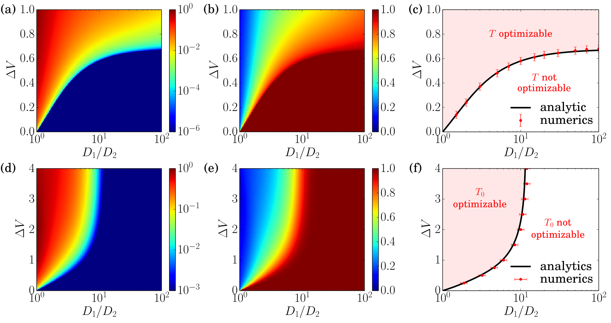
Figure 7: MFPT optimization in 2d for ε=0.1\varepsilon=0.1. (a) and (d) Difference between the minimal GMFPT/CMFPT and the GMFPT/CMFPT for the disk geometry: T⁡(χ∗)−T⁡(0)T(\chi_{*})-T(0) (resp. T0​(χ∗)−T0​(0)T_{0}(\chi_{*})-T_{0}(0)) as a function of D1/D2D_{1}/D_{2} and β​Δ​V\beta\Delta V, calculated with the narrow escape expression given by Eqs. (35) and (36) respectively. (b) and (e) Corresponding widths Δ∗/ℛ=1−χ∗\Delta_{*}/{\cal R}=1-\chi_{*} for which the GMFPT/CMFPT is minimal, as a function of D1/D2D_{1}/D_{2} and β​Δ​V\beta\Delta V. (c) and (f) GMFPT/CMFPT optimization diagrams deduced from the numerical solutions obtained with the finite element method using FreeFem++ (dots) and the analytical condition given by Eqs. (44) and (48) respectively.

Fig. 7(a) shows the difference between the minimal GMFPT T⁡(χ∗)T(\chi_{*}) and the GMFPT for the disk geometry T⁡(0)=−ln⁡(ε/4)+1/8T(0)=-\ln(\varepsilon/4)+1/8 as a function of D1/D2>1D_{1}/D_{2}>1 and β​Δ​V>0\beta\Delta V>0 for an escape angle ε=0.1\varepsilon=0.1. In other quadrants this minimal value is zero for D1>D2D_{1}>D_{2} and Δ​V<0\Delta V<0, or T⁡(1)−T⁡(0)=(D1/D2−1)​T​(0)T(1)-T(0)=(D_{1}/D_{2}-1)T(0) for D1<D2D_{1}<D_{2}, considering the Eq. (15). The GMFPT can be minimized for D1=D2D_{1}=D_{2} and Δ​V>0\Delta V>0 leading to a discontinuity of this minimal MFPT between the different quadrants. Fig. 7(b) displays the corresponding width Δ∗/ℛ\Delta_{*}/{\cal R} for which the minimum of the GMFPT is attained. Finally Fig. 7(c) shows the GMFPT optimization diagram derived from Eq. (44) and the numerical solutions (dots). For β​Δ​V>0.68\beta\Delta V>0.68 the GMFPT is always optimizable, a value which depends on ε\varepsilon as ln⁡|T∗/(T∗−2)|\ln\left|T_{*}/(T_{*}-2)\right|.

For the CMFPT, the Taylor expansion of Eq. (36) at χ=0\chi=0 gives

T0​(χ)=−ln⁡ε4+14+χ2​{(ξ−1)​[−ln⁡ε4−12​ln⁡χ]+2​D1−D2​ξD1+D2​ξ+D1−D24​D2}+𝒪⁡(χ4).\displaystyle T_{0}(\chi)=-\ln\frac{\varepsilon}{4}+\frac{1}{4}+\chi^{2}\left\{(\xi-1)\left[-\ln\frac{\varepsilon}{4}-\frac{1}{2}\ln\chi\right]+2\frac{D_{1}-D_{2}\xi}{D_{1}+D_{2}\xi}+\frac{D_{1}-D_{2}}{4D_{2}}\right\}+{\cal O}(\chi^{4}). (46)

The optimization is then possible if and only if T0​(χ)−T0​(0)<0T_{0}(\chi)-T_{0}(0)<0 considering all the leading terms in the narrow escape limit and corresponding terms in the Taylor expansion, i.e. assuming that ln⁡ε\ln\varepsilon and ln⁡χ\ln\chi are of same order for a value χ=χ0≪1\chi=\chi_{0}\ll 1. We obtain then the condition

(ξ−1)​T∗+2​D1−D2​ξD1+D2​ξ+D1−D24​D2<0,T∗=−ln⁡ε4−12​ln⁡χ0,(\xi-1)T_{*}+2\frac{D_{1}-D_{2}\xi}{D_{1}+D_{2}\xi}+\frac{D_{1}-D_{2}}{4D_{2}}<0,\qquad T_{*}=-\ln\frac{\varepsilon}{4}-\frac{1}{2}\ln\chi_{0}, (47)

where χ0\chi_{0} is to be determined. This condition is satisfied for

ξ<(D2−D1)​T∗+2​D2+D2−D14+[(D2−D1)​T∗+2​D2+D2−D14]2−4​D1​D2​(2−T∗+D1−D24​D2)​T∗2​D2​T∗.\xi<\frac{(D_{2}-D_{1})T_{*}+2D_{2}+\frac{D_{2}-D_{1}}{4}+\sqrt{\left[(D_{2}-D_{1})T_{*}+2D_{2}+\frac{D_{2}-D_{1}}{4}\right]^{2}-4D_{1}D_{2}\left(2-T_{*}+\frac{D_{1}-D_{2}}{4D_{2}}\right)T_{*}}}{2D_{2}T_{*}}. (48)

In the limit ε≪1\varepsilon\ll 1, T∗T_{*} diverges and the last condition can be rewritten as

β​Δ​V>(D1−D2)​(D1+9​D2)4​D2​(D1+D2)​T∗+𝒪⁡(T∗−2).\beta\Delta V>\frac{(D_{1}-D_{2})(D_{1}+9D_{2})}{4D_{2}(D_{1}+D_{2})T_{*}}+{\cal O}(T_{*}^{-2}). (49)

Fig. 7(d) shows the difference between the minimal CMFPT T0​(χ∗)T_{0}(\chi_{*}) and the CMFPT for the disk geometry T0​(0)=−ln⁡(ε/4)+1/4T_{0}(0)=-\ln(\varepsilon/4)+1/4 as a function of D1/D2>1D_{1}/D_{2}>1 and β​Δ​V>0\beta\Delta V>0 for an escape angle ε=0.1\varepsilon=0.1. In other quadrants this minimal value is (D1/D2−1)​T0​(0)(D_{1}/D_{2}-1)T_{0}(0) (for D1<D2D_{1}<D_{2}) or zero. Fig. 7(e) displays the corresponding width Δ∗/ℛ\Delta_{*}/{\cal R} for which the minimum of the CMFPT is attained. Finally Fig. 7(f) shows the CMFPT optimization diagram derived from Eq. (48) and the numerical solutions (dots). The numerical solution yields χ0≃exp⁡(−2)≃0.13\chi_{0}\simeq\exp(-2)\simeq 0.13 (independent of ε\varepsilon) which implies T∗=−ln⁡(ε/4)+1T_{*}=-\ln(\varepsilon/4)+1. Additionally for D1/D2>11.75D_{1}/D_{2}>11.75 the CMFPT is never optimizable, a value which depends on ε\varepsilon as −7+4​T∗-7+4T_{*}. In fact the right hand side of Eq. (48) becomes negative implying that ξ\xi needs to be negative to have a CMFPT optimization which cannot be satisfied.

V.2 Narrow escape limit in three dimensions

In appendix B we show that close to the escape region the 3d Green’s function behaves as

G⁡(𝐱→𝐱𝟎|𝐱𝟎)=12​π​D​(𝐱𝟎)​1|𝐱−𝐱𝟎|+γ​ln⁡|𝐱−𝐱𝟎|2​ℛ+R0,G({\bf x}\rightarrow{\bf x_{0}}|{\bf x_{0}})=\frac{1}{2\pi D({\bf x_{0}})}\frac{1}{|{\bf x}-{\bf x_{0}}|}+\gamma\ln\frac{|{\bf x}-{\bf x_{0}}|}{2{\cal R}}+R_{0}, (50)

where γ\gamma and R0R_{0} are respectively the logarithmic diverging and regular parts of the pseudo Green’s function at the center of the escape region and the average MFPT verifies the expression

⟨t⟩=1Ps​(𝐱𝟎)​[12​D​(𝐱𝟎)​ℛ​ε+γ​ln⁡ε+R0−32​γ].\langle t\rangle=\frac{1}{P_{s}({\bf x_{0}})}\left[\frac{1}{2D({\bf x_{0}}){\cal R}\varepsilon}+\gamma\ln\varepsilon+R_{0}-\frac{3}{2}\gamma\right]. (51)

In the appendix D we derive the pseudo Green’s function and identify γ\gamma and R0R_{0}. The dimensionless GMFPT is

T⁡(χ)=D1​⟨t⟩ℛ2=[1−χ3​(1−ξ)]​{2​π3​ε−13​ln⁡ε+13​∑n=1∞(2​n+1)2n⁡(n+1)​un​χ2​n+11−un​χ2​n+1−16}\displaystyle T(\chi)=\frac{D_{1}\langle t\rangle}{{\cal R}^{2}}=\left[1-\chi^{3}(1-\xi)\right]\left\{\frac{2\pi}{3\varepsilon}-\frac{1}{3}\ln\varepsilon+\frac{1}{3}\sum_{n=1}^{\infty}\frac{(2n+1)^{2}}{n(n+1)}\frac{u_{n}\chi^{2n+1}}{1-u_{n}\chi^{2n+1}}-\frac{1}{6}\right\}
+D2+[(D1−D2)​ξ+4​D2​(1−ξ)+5​D2​(1−ξ)2]​χ515​D2​[1−χ3​(1−ξ)]−(1−ξ)​[1+χ3​(1−ξ)]3​[1−χ3​(1−ξ)]​χ3,\displaystyle+\frac{D_{2}+[(D_{1}-D_{2})\xi+4D_{2}(1-\xi)+5D_{2}(1-\xi)^{2}]\chi^{5}}{15D_{2}\left[1-\chi^{3}(1-\xi)\right]}-\frac{(1-\xi)\left[1+\chi^{3}(1-\xi)\right]}{3\left[1-\chi^{3}(1-\xi)\right]}\chi^{3}, (52)

with χ=1−Δ/ℛ\chi=1-\Delta/{\cal R}, ξ=exp⁡(−β​Δ​V)\xi=\exp(-\beta\Delta V) and the sequence

un=(n+1)​(D1−D2​ξ)(n+1)​D1+n​D2​ξ,u_{n}=\frac{(n+1)(D_{1}-D_{2}\xi)}{(n+1)D_{1}+nD_{2}\xi}, (53)

and the dimensionless CMFPT is

T0​(χ)=D1​t​(𝟎)ℛ2=[1−χ3​(1−ξ)]​{2​π3​ε−13​ln⁡ε+13​∑n=1∞(2​n+1)2n⁡(n+1)​un​χ2​n+11−un​χ2​n+1−16}\displaystyle T_{0}(\chi)=\frac{D_{1}t({\bf 0})}{{\cal R}^{2}}=\left[1-\chi^{3}(1-\xi)\right]\left\{\frac{2\pi}{3\varepsilon}-\frac{1}{3}\ln\varepsilon+\frac{1}{3}\sum_{n=1}^{\infty}\frac{(2n+1)^{2}}{n(n+1)}\frac{u_{n}\chi^{2n+1}}{1-u_{n}\chi^{2n+1}}-\frac{1}{6}\right\}
+16+D1−D26​D2​χ2−1−ξ3​χ2​(1−χ).\displaystyle+\frac{1}{6}+\frac{D_{1}-D_{2}}{6D_{2}}\chi^{2}-\frac{1-\xi}{3}\chi^{2}(1-\chi). (54)

Consequently, the GMFPT and the CMFPT can be written as the sum of two terms: (i) the first line of each expression is common and contains the leading order [1−χ3​(1−ξ)]​[2​π/3​ε−ln⁡ε/3−1/6][1-\chi^{3}(1-\xi)][2\pi/3\varepsilon-\ln\varepsilon/3-1/6] and (ii) the second line is the corresponding MFPT for a fully absorbing external boundary (ε=2​π\varepsilon=2\pi), see the derivation in the appendix F. Note that the series in common term is zero when β​Δ​V=ln⁡(D2/D1)\beta\Delta V=\ln(D_{2}/D_{1}) as for 2d NEP. From Eqs. (52) and (54), we recover the expressions for the sphere geometry cheviakov2010 when D1=D2D_{1}=D_{2} and Δ​V=0\Delta V=0:

T=2​π3​ε−13​ln⁡ε−110,T0=2​π3​ε−13​ln⁡ε;T=\frac{2\pi}{3\varepsilon}-\frac{1}{3}\ln\varepsilon-\frac{1}{10},\qquad T_{0}=\frac{2\pi}{3\varepsilon}-\frac{1}{3}\ln\varepsilon; (55)

and we mention two other interesting cases studied in 2d in Ref. mangeat2019: (i) the narrow escape limit for the annulus geometry when Δ​V→+∞\Delta V\to+\infty:

T⁡(χ)=(1−χ3)​[2​π3​ε−13​ln⁡ε+13​∑n=1∞(2​n+1)2n⁡(n+1)​χ2​n+11−χ2​n+1]−1−6​χ5+5​χ610​(1−χ3),\displaystyle T(\chi)=(1-\chi^{3})\left[\frac{2\pi}{3\varepsilon}-\frac{1}{3}\ln\varepsilon+\frac{1}{3}\sum_{n=1}^{\infty}\frac{(2n+1)^{2}}{n(n+1)}\frac{\chi^{2n+1}}{1-\chi^{2n+1}}\right]-\frac{1-6\chi^{5}+5\chi^{6}}{10(1-\chi^{3})}, (56)
T0​(χ)=(1−χ3)​[2​π3​ε−13​ln⁡ε+13​∑n=1∞(2​n+1)2n⁡(n+1)​χ2​n+11−χ2​n+1]+D1−D26​D2​χ2−χ26​(2−3​χ);\displaystyle T_{0}(\chi)=(1-\chi^{3})\left[\frac{2\pi}{3\varepsilon}-\frac{1}{3}\ln\varepsilon+\frac{1}{3}\sum_{n=1}^{\infty}\frac{(2n+1)^{2}}{n(n+1)}\frac{\chi^{2n+1}}{1-\chi^{2n+1}}\right]+\frac{D_{1}-D_{2}}{6D_{2}}\chi^{2}-\frac{\chi^{2}}{6}(2-3\chi); (57)

and (ii) the narrow escape limit for the two-shell geometry with heterogeneous diffusivity when Δ​V=0\Delta V=0:

T⁡(χ)=2​π3​ε−13​ln⁡ε+13​∑n=1∞(2​n+1)2n⁡(n+1)​un​χ2​n+11−un​χ2​n+1−16+D2+(D1−D2)​χ515​D2,\displaystyle T(\chi)=\frac{2\pi}{3\varepsilon}-\frac{1}{3}\ln\varepsilon+\frac{1}{3}\sum_{n=1}^{\infty}\frac{(2n+1)^{2}}{n(n+1)}\frac{u_{n}\chi^{2n+1}}{1-u_{n}\chi^{2n+1}}-\frac{1}{6}+\frac{D_{2}+(D_{1}-D_{2})\chi^{5}}{15D_{2}}, (58)
T0​(χ)=2​π3​ε−13​ln⁡ε+13​∑n=1∞(2​n+1)2n⁡(n+1)​un​χ2​n+11−un​χ2​n+1+D1−D26​D2​χ2.\displaystyle T_{0}(\chi)=\frac{2\pi}{3\varepsilon}-\frac{1}{3}\ln\varepsilon+\frac{1}{3}\sum_{n=1}^{\infty}\frac{(2n+1)^{2}}{n(n+1)}\frac{u_{n}\chi^{2n+1}}{1-u_{n}\chi^{2n+1}}+\frac{D_{1}-D_{2}}{6D_{2}}\chi^{2}. (59)
Figure 8: Dependence of the dimensionless GMFPT (a) and CMFPT (b) on the escape angle ε\varepsilon in 3d for several widths Δ/ℛ\Delta/{\cal R} and fixed parameters D1/D2=5D_{1}/D_{2}=5 and β​Δ​V=2\beta\Delta V=2. The symbols show the numerical solution obtained with the finite element method using FreeFem++ and the lines display the analytical expressions given by Eqs. (52) and (54) in the narrow escape limit. (c) Correction to the leading term D1​R0D_{1}R_{0} for the unit sphere ℛ=1{\cal R}=1 as a function of Δ/ℛ\Delta/{\cal R} for fixed parameters D1/D2=5D_{1}/D_{2}=5 and β​Δ​V=2\beta\Delta V=2. The circles represent the fitted value, extracted from numerical solutions with Eq. (51), while the line shows the analytical solution from Eq. (52). The squares display the relative difference between the numerical fit and the analytical expression.

Figs. 8(a) and 8(b) display the dependence of the GMFPT and the CMFPT, respectively, on the escape angle for several widths of the outer shell Δ\Delta and the fixed parameters D1/D2=5D_{1}/D_{2}=5 and β​Δ​V=2\beta\Delta V=2. The analytical expressions (lines) given by Eqs. (52) and (54) match the numerical solutions (symbols) in the narrow escape limit. The two MFPTs show the same hyperbolic decrease in ε\varepsilon, already observed in Fig. 3(b), and the accuracy of the narrow escape expressions increases with Δ\Delta. Fig. 8(c) shows the correction to the leading order D1​R0D_{1}R_{0} defined as the regular part of the Green’s function (for the unit sphere) at the center of the escape region and extracted numerically (circles) from a regression analysis of numerical solutions of GMFPT as a function of ε\varepsilon by using Eq. (51). Comparing it with analytical expression derived in appendix D (line), the maximal relative error is smaller than 3% (squares), except for Δ∼0.4​ℛ\Delta\sim 0.4{\cal R} when R0R_{0} crosses 00. Note that the second order sub-leading corrections (instead of first order in two dimensions) are compared and the accumulated numerical error is less than 10−410^{-4}.

Figure 9: Dependence of the dimensionless GMFPT [(a) and (c)] and CMFPT [(b) and (d)] on the width Δ/ℛ\Delta/{\cal R} in 3d for several potential differences β​Δ​V\beta\Delta V, the escape angle ε=0.1\varepsilon=0.1 and the ratio of diffusion constants D1/D2=5D_{1}/D_{2}=5 [(a) and (b)] and D1/D2=0.2D_{1}/D_{2}=0.2 [(c) and (d)]. The symbols display the numerical solutions obtained with the finite element method using FreeFem++ and the lines show the analytical expressions given by Eqs. (52) and (54) for the GMFPT and the CMFPT respectively, in the narrow escape limit (here for Δ\Delta close to ℛ{\cal R}). The dash-dotted lines display the Δ→0\Delta\to 0 limit given by Eq. (16). In insets, the same curves are shown in linear scale for a better observation of the minima exhibited by the GMFPT and the CMFPT.

Fig. 9 shows the dependence of the GMFPT and the CMFPT on the width of the outer shell Δ\Delta for fixed escape angle ε=0.1\varepsilon=0.1. The numerical solutions (symbols) agree well with the narrow escape expressions (lines) given by Eqs. (52) and (54) for Δ\Delta close to ℛ{\cal R} and approach the thin cortex expressions (dash-dotted lines) given by Eq. (16) in the Δ→0\Delta\to 0 limit. In Figs. 9(a) and 9(b) for a larger diffusion constant in the cortex D1/D2=5D_{1}/D_{2}=5, the GMFPT has a minimum for β​Δ​V>0.05\beta\Delta V>0.05 and the CMFPT for β​Δ​V>0.14\beta\Delta V>0.14 compatible with the inset. The minima are perfectly described by the narrow escape expressions as for 2d NEP. However, in Figs. 9(c) and 9(d) for a smaller diffusion constant in the cortex D1/D2=0.2D_{1}/D_{2}=0.2 the value of the GMFPT and the CMFPT for Δ=0\Delta=0 is always smaller than for Δ=ℛ\Delta={\cal R} due to the fast motion in the central region, consistent with the relation (15) derived in Sec. III. This implies that the MFPT is always minimal for Δ=0\Delta=0 when D1<D2D_{1}<D_{2}.

As for the 2d case, we focus on D1>D2D_{1}>D_{2} for which the MFPT can be optimized for a width 0<Δ<ℛ0<\Delta<{\cal R}. For the GMFPT, the Taylor expansion of Eq. (52) at χ=0\chi=0 gives

T⁡(χ)=2​π3​ε−13​ln⁡ε−110+χ3​{(ξ−1)​[2​π3​ε−13​ln⁡ε+110]+3​D1−D2​ξ2​D1+D2​ξ}+𝒪⁡(χ5).T(\chi)=\frac{2\pi}{3\varepsilon}-\frac{1}{3}\ln\varepsilon-\frac{1}{10}+\chi^{3}\left\{(\xi-1)\left[\frac{2\pi}{3\varepsilon}-\frac{1}{3}\ln\varepsilon+\frac{1}{10}\right]+3\frac{D_{1}-D_{2}\xi}{2D_{1}+D_{2}\xi}\right\}+{\cal O}(\chi^{5}). (60)

The optimization is then possible if and only if T⁡(χ)−T⁡(0)<0T(\chi)-T(0)<0 or

(ξ−1)​T∗+3​D1−D2​ξ2​D1+D2​ξ<0,T∗=2​π3​ε−13​ln⁡ε+110.(\xi-1)T_{*}+3\frac{D_{1}-D_{2}\xi}{2D_{1}+D_{2}\xi}<0,\qquad T_{*}=\frac{2\pi}{3\varepsilon}-\frac{1}{3}\ln\varepsilon+\frac{1}{10}. (61)

This condition is satisfied for

ξ<(D2−2​D1)​T∗+3​D2+[(D2−2​D1)​T∗+3​D2]2−4​D1​D2​(3−2​T∗)​T∗2​D2​T∗.\xi<\frac{(D_{2}-2D_{1})T_{*}+3D_{2}+\sqrt{[(D_{2}-2D_{1})T_{*}+3D_{2}]^{2}-4D_{1}D_{2}(3-2T_{*})T_{*}}}{2D_{2}T_{*}}. (62)

In the limit ε≪1\varepsilon\ll 1, T∗T_{*} diverges and the last condition can be rewritten as

β​Δ​V>3​(D1−D2)(2​D1+D2)​T∗+𝒪⁡(T∗−2).\beta\Delta V>\frac{3(D_{1}-D_{2})}{(2D_{1}+D_{2})T_{*}}+{\cal O}(T_{*}^{-2}). (63)
Refer to caption
Figure 10: MFPT optimization in 3d for ε=0.5\varepsilon=0.5. (a) and (d) Difference between the minimal GMFPT/CMFPT and the GMFPT/CMFPT for the disk geometry: T⁡(χ∗)−T⁡(0)T(\chi_{*})-T(0) (resp. T0​(χ∗)−T0​(0)T_{0}(\chi_{*})-T_{0}(0)) as a function of D1/D2D_{1}/D_{2} and β​Δ​V\beta\Delta V, calculated from the narrow escape expression given by Eqs. (52) and (54) respectively. (b) and (e) Corresponding widths Δ∗/ℛ=1−χ∗\Delta_{*}/{\cal R}=1-\chi_{*} for which the GMFPT/CMFPT is minimal, as a function of D1/D2D_{1}/D_{2} and β​Δ​V\beta\Delta V. (c) and (f) GMFPT/CMFPT optimization diagrams deduced from the numerical solutions obtained with the finite element method using FreeFem++ (dots) and the analytical condition given by Eqs. (62) and (66) respectively.

Fig. 10(a) displays the difference between the minimal GMFPT T⁡(χ∗)T(\chi_{*}) and the GMFPT for the disk geometry T⁡(0)=2​π/3​ε−ln⁡ε/3−1/10T(0)=2\pi/3\varepsilon-\ln\varepsilon/3-1/10 as a function of D1/D2>1D_{1}/D_{2}>1 and β​Δ​V>0\beta\Delta V>0 for an escape angle ε=0.5\varepsilon=0.5. In other quadrants this minimal value is (D1/D2−1)​T​(0)(D_{1}/D_{2}-1)T(0) (for D1<D2D_{1}<D_{2}) or zero. Fig. 10(b) shows the corresponding width Δ∗/ℛ\Delta_{*}/{\cal R} for which the minimum of the GMFPT is attained. Finally Fig. 10(c) displays the GMFPT optimization diagram derived from Eq. (62) and the numerical solutions (dots). For β​Δ​V>0.40\beta\Delta V>0.40 the GMFPT is always optimizable, a value which depends on ε\varepsilon as ln⁡|2​T∗/(2​T∗−3)|\ln\left|2T_{*}/(2T_{*}-3)\right|.

For the CMFPT, the Taylor expansion of Eq. (54) at χ=0\chi=0 gives

T0​(χ)=2​π3​ε−13​ln⁡ε+χ23​[D1−D22​D2−1+ξ]+χ3​{(ξ−1)​[2​π3​ε−13​ln⁡ε−12]+3​D1−D2​ξ2​D1+D2​ξ}+𝒪⁡(χ5).\displaystyle T_{0}(\chi)=\frac{2\pi}{3\varepsilon}-\frac{1}{3}\ln\varepsilon+\frac{\chi^{2}}{3}\left[\frac{D_{1}-D_{2}}{2D_{2}}-1+\xi\right]+\chi^{3}\left\{(\xi-1)\left[\frac{2\pi}{3\varepsilon}-\frac{1}{3}\ln\varepsilon-\frac{1}{2}\right]+3\frac{D_{1}-D_{2}\xi}{2D_{1}+D_{2}\xi}\right\}+{\cal O}(\chi^{5}). (64)

The optimization is then possible if and only if T0​(χ)−T0​(0)<0T_{0}(\chi)-T_{0}(0)<0 considering all the leading terms in the narrow escape limit and corresponding terms in the Taylor expansion, i.e. assuming that ε−1\varepsilon^{-1} and χ−1\chi^{-1} are of same order for a value χ=χ0≪1\chi=\chi_{0}\ll 1. We obtain then the condition

(ξ−1)​T∗+D1−D26​D2​χ0+3​D1−D2​ξ2​D1+D2​ξ<0,T∗=2​π3​ε−13​ln⁡ε−12+13​χ0.(\xi-1)T_{*}+\frac{D_{1}-D_{2}}{6D_{2}\chi_{0}}+3\frac{D_{1}-D_{2}\xi}{2D_{1}+D_{2}\xi}<0,\qquad T_{*}=\frac{2\pi}{3\varepsilon}-\frac{1}{3}\ln\varepsilon-\frac{1}{2}+\frac{1}{3\chi_{0}}. (65)

where χ0\chi_{0} is to be determined. This condition is satisfied for

ξ<(D2−2​D1)​T∗+3​D2−D1−D26​χ0+[(D2−2​D1)​T∗+3​D2−D1−D26​χ0]2−4​D1​D2​(3−2​T∗+D1−D23​D2​χ0)​T∗2​D2​T∗.\xi<\frac{(D_{2}-2D_{1})T_{*}+3D_{2}-\frac{D_{1}-D_{2}}{6\chi_{0}}+\sqrt{\left[(D_{2}-2D_{1})T_{*}+3D_{2}-\frac{D_{1}-D_{2}}{6\chi_{0}}\right]^{2}-4D_{1}D_{2}\left(3-2T_{*}+\frac{D_{1}-D_{2}}{3D_{2}\chi_{0}}\right)T_{*}}}{2D_{2}T_{*}}. (66)

In the limit ε≪1\varepsilon\ll 1, T∗T_{*} diverges and the last condition can be rewritten as

β​Δ​V>3​(D1−D2)(2​D1+D2)​T∗+D1−D26​D2​T∗​χ0+𝒪⁡(T∗−2).\beta\Delta V>\frac{3(D_{1}-D_{2})}{(2D_{1}+D_{2})T_{*}}+\frac{D_{1}-D_{2}}{6D_{2}T_{*}\chi_{0}}+{\cal O}(T_{*}^{-2}). (67)

Numerically we have identified the constant χ0≃0.4\chi_{0}\simeq 0.4.

Fig. 10(d) shows the difference between the minimal CMFPT T0​(χ∗)T_{0}(\chi_{*}) and the CMFPT for the disk geometry T0​(0)=2​π/3​ε−ln⁡ε/3T_{0}(0)=2\pi/3\varepsilon-\ln\varepsilon/3 as a function of D1/D2>1D_{1}/D_{2}>1 and β​Δ​V>0\beta\Delta V>0 for an escape angle ε=0.5\varepsilon=0.5. In other quadrants this minimal value is (D1/D2−1)​T0​(0)(D_{1}/D_{2}-1)T_{0}(0) (for D1<D2D_{1}<D_{2}) or zero. Fig. 10(e) displays the corresponding width Δ∗/ℛ\Delta_{*}/{\cal R} for which the minimum of the CMFPT is attained. Note that in contrast to the 2d case Δ∗\Delta_{*} changes abruptly, apparently discontinuously, when going from the left region (blue) to the right region (red), where Δ∗=ℛ\Delta_{*}={\cal R}. Finally Fig. 10(f) shows the CMFPT optimization diagram from Eq. (66) and the numerical solutions (dots). The numerical solution yields χ0≃0.4\chi_{0}\simeq 0.4 (independent of ε\varepsilon). Additionally for D1/D2>0.81D_{1}/D_{2}>0.81 the CMFPT is never optimizable, a value which depends on ε\varepsilon as 1+(−9+6​T∗)​χ01+(-9+6T_{*})\chi_{0}. In fact the right hand side of Eq. (66) becomes negative implying that ξ\xi needs to be negative to have a CMFPT optimization which cannot be satisfied.

VI Discussion

Figure 11: Dependence of the dimensionless GMFPT (a) and CMFPT (b) on the width Δ/ℛ\Delta/{\cal R} in 2d for the escape angle ε=0.1\varepsilon=0.1, different ratios of diffusion constants D1/D2D_{1}/D_{2} and a difference potential β​Δ​V=ln⁡(D2/D1)\beta\Delta V=\ln(D_{2}/D_{1}). The symbols show the numerical solutions obtained with the finite element method using FreeFem++ and the lines display the exact analytical expressions given by Eqs. (68) and (69) for the GMFPT and the CMFPT respectively.

In Sec. III we have derived the thin cortex limit of the MFPT given by Eqs. (16) and (20) for respectively Δ​V<+∞\Delta V<+\infty and exp⁡(−β​Δ​V)=0\exp(-\beta\Delta V)=0 (annulus geometry), which are both particular solutions of the SMDP. In Secs. IV and V we have analyzed the evolution of the GMFPT and the CMFPT according to four parameters: the escape angle ε\varepsilon, the width of the outer shell Δ/ℛ\Delta/{\cal R}, the ratio of diffusion constants D1/D2D_{1}/D_{2} and the potential difference Δ​V\Delta V. The dimensionless MFPT D1​t​(𝐱)/ℛ2D_{1}t({\bf x})/{\cal R}^{2} is a decreasing function of ε\varepsilon and Δ​V\Delta V and an increasing function of D1/D2D_{1}/D_{2}, from simple arguments. However the behavior of the MFPT (as well as GMFPT or CMFPT) can be non-monotonous with Δ/ℛ\Delta/{\cal R}. For diffusion constants D1<D2D_{1}<D_{2}, the particles move faster to the escape region when the central region is as large as possible, which implies a minimum of GMFPT/CMFPT when Δ=0\Delta=0 compatible with the relation (15) in the thin cortex limit. For the opposite situation (D1>D2D_{1}>D_{2}) the presence of an optimization depends on the potential difference. If the cortex is repulsive (Δ​V<0\Delta V<0) the particle moves faster when it is not energetically trapped in the central region, which implies a minimum of GMFPT/CMFPT when Δ=ℛ\Delta={\cal R}. Finally in the last quadrant (D1>D2D_{1}>D_{2} and Δ​V>0\Delta V>0) the GMFPT/CMPFT can be optimized due to the competition between the attractiveness of cortex (energetic trap) and the slower diffusion in the central region (diffusive trap). In Sec. V we have derived an analytical expression for both the GMFPT and the CMFPT in the narrow escape limit (ε≪1\varepsilon\ll 1) in 2d and 3d. These expressions yield a quantitative condition for the potential difference for the MFPT optimization with a width 0<Δ∗<ℛ0<\Delta_{*}<{\cal R}. Nevertheless we did not derive an analytical expression for Δ∗=(1−χ∗)​ℛ\Delta_{*}=(1-\chi_{*}){\cal R} as well as T⁡(χ∗)T(\chi_{*}) and T0​(χ∗)T_{0}(\chi_{*}) due to the complexity of the narrow escape expressions and the rapidity to obtain them numerically (see Figs. 7 and 10).

Finally we look more precisely at the special case β​V​(𝐱)=ln⁡D⁡(𝐱)\beta V({\bf x})=\ln D({\bf x}). With this potential, the flux of Brownian particles is equal to −∇𝐱[D⁡(𝐱)​p​(𝐱,t)]-\nabla_{\bf x}\left[D({\bf x})p({\bf x},t)\right] and the convective term in the Itô convention, given by Eq. (26), is zero. The MFPT then obeys the Poisson’s equation ∇𝐱2t(𝐱)=−1/D(𝐱)\nabla_{\bf x}^{2}t({\bf x})=-1/D({\bf x}). A recent study reported an exact solution for this equation in arbitrary two dimensional connected domains grebenkov2016. In appendix E we derive from this result an exact solution of the MFPT in the two-shell geometry for which β​Δ​V=ln⁡(D2/D1)\beta\Delta V=\ln(D_{2}/D_{1}). In particular, the GMFPT is

T=−(1+D1−D2D2​χ2)​ln⁡sin⁡(ε/4)+18+D1−D28​D2​3​D2+(D1−3​D2)​χ2D2+(D1−D2)​χ2​χ2−(D1−D2)22​D2​χ4​ln⁡χD2+(D1−D2)​χ2,T=-\left(1+\frac{D_{1}-D_{2}}{D_{2}}\chi^{2}\right)\ln\sin(\varepsilon/4)+\frac{1}{8}+\frac{D_{1}-D_{2}}{8D_{2}}\frac{3D_{2}+(D_{1}-3D_{2})\chi^{2}}{D_{2}+(D_{1}-D_{2})\chi^{2}}\chi^{2}-\frac{(D_{1}-D_{2})^{2}}{2D_{2}}\frac{\chi^{4}\ln\chi}{D_{2}+(D_{1}-D_{2})\chi^{2}}, (68)

and the CMFPT is

T0=−(1+D1−D2D2​χ2)​ln⁡sin⁡(ε/4)+14+D1−D24​D2​χ2+D2−D12​D2​χ2​ln⁡χ.T_{0}=-\left(1+\frac{D_{1}-D_{2}}{D_{2}}\chi^{2}\right)\ln\sin(\varepsilon/4)+\frac{1}{4}+\frac{D_{1}-D_{2}}{4D_{2}}\chi^{2}+\frac{D_{2}-D_{1}}{2D_{2}}\chi^{2}\ln\chi. (69)

These two expressions are exact for all values of ε\varepsilon, χ=1−Δ/ℛ\chi=1-\Delta/{\cal R} and D1/D2D_{1}/D_{2}, and are compatible with Eqs. (35) and (36) for β​Δ​V=ln⁡(D2/D1)\beta\Delta V=\ln(D_{2}/D_{1}) in the limit ε≪1\varepsilon\ll 1 (where sin⁡(ε/4)≃ε/4\sin(\varepsilon/4)\simeq\varepsilon/4). Note that the series in Eqs. (35) and (36) is zero only for this potential difference. The thin cortex limits (i.e. χ=1\chi=1) are consistent with Eqs. (15) and (16).

The GMFPT and CMPFT are decreasing functions of the escape angle ε\varepsilon and of the ratio of diffusion constants D1/D2D_{1}/D_{2}. Fig. 11 displays the dependence of the GMFPT and the CMFPT on the width of the outer shell Δ\Delta for ε=0.1\varepsilon=0.1 and several ratios D1/D2D_{1}/D_{2}. The analytical expressions given by Eqs. (68) and (69) match perfectly the numerical solutions for all values of Δ\Delta. For D1>D2D_{1}>D_{2}, the potential difference is negative and the GMFPT/CMFPT is a decreasing function of Δ\Delta leading to a minimum MFPT located at Δ=ℛ\Delta={\cal R}. For D1<D2D_{1}<D_{2}, the potential difference is positive and the GMFPT/CMFPT is an increasing function of Δ\Delta resulting in a minimal MFPT for Δ=0\Delta=0. Unfortunately, the interesting range of parameters (D1>D2D_{1}>D_{2} and Δ​V>0\Delta V>0), which allows an optimization of the MFPT with Δ>0\Delta>0, is not attained for this particular potential difference.

To conclude we have characterized the MFPT for passive Brownian particles to reach a small escape window within the two-shell geometry in which the particles diffuse in each shell with different diffusive constant, with a potential barrier between the two shells. We have derived asymptotic expressions of the MFPT in the thin cortex and the narrow escape limits and we have obtained an exact solution only for one particular relation of the potential difference with the ratio of diffusion constants. For the most interesting case, showing a higher diffusion in the attractive cortex, we have derived from the narrow escape expressions a condition on the potential difference to have a MFPT optimization for particles starting from a random position or from the center. The potential barrier pushing the particles towards the surface needs to be large enough to balance the slowing down of the diffusion within the central region. With this result we may better understand the presence of a minimum for the intracellular transport time since the effective diffusivity is higher in the actin cortex, and the ballistic transport on filaments favors the transport to the cell membrane. Since the cargo particles perform an intermittent search, we may imagine that the MFPT is strongly reduced compared to our passive Brownian motion and that a condition on switching rates and ballistic velocity will replace the condition on the potential difference to have a MFPT optimization.

An interesting perspective would be to derive an exact expression for the GMFPT or the CMFPT, corresponding to the one derived in Ref. grebenkov2016, as well as for the optimized MFPT. Moreover, it would be interesting to derive a condition for an optimized intracellular transport time by reintroducing an intermittent ballistic transport for which, to our knowledge, no analytical expression has been reported so far. Finally another interesting perspective would be the study of the distribution of first passage time, and check whether the MFPT is relevant and close to the typical first passage time.

VII Acknowledgement

This work was performed with financial support from the German Research Foundation (DFG) within the Collaborative Research Center SFB 1027.

Appendix A The thin cortex limit

A.1 Link with the surface-mediated diffusion problem

From Eqs. (6) and (11), the bulk MFPT tBt_{\rm B} can be identified with the MFPT t2t_{2} when Δ→0\Delta\rightarrow 0 whereas the MFPT t1​(r,θ)t_{1}(r,\theta) can be expanded in the radial coordinate as

t1​(r,θ)=f0​(θ)+(r−ℛ)​f1​(θ)+(r−ℛ)22​f2​(θ)+⋯t_{1}(r,\theta)=f_{0}(\theta)+(r-{\cal R})f_{1}(\theta)+\frac{(r-{\cal R})^{2}}{2}f_{2}(\theta)+\cdots (70)

Using Eq. (8), the reflective boundary condition ∂rt1​(ℛ,θ)=0\partial_{r}t_{1}({\cal R},\theta)=0 gives f1​(θ)=0f_{1}(\theta)=0 while the absorbing boundary condition t1​(ℛ,θ)=0t_{1}({\cal R},\theta)=0 yields f0​(θ)=0f_{0}(\theta)=0 for |θ|<ε/2|\theta|<\varepsilon/2. In leading order in the Δ≪ℛ\Delta\ll{\cal R} expansion, we can then set f0​(θ)=tΣ​(θ)f_{0}(\theta)=t_{\Sigma}(\theta). Eq. (5) can then be written as

D1​[∂2t1∂r2​(r,θ)+d−1r​∂t1∂r​(r,θ)+1r2​Δθ​t1​(r,θ)]=−1,D_{1}\left[\frac{\partial^{2}t_{1}}{\partial r^{2}}(r,\theta)+\frac{d-1}{r}\frac{\partial t_{1}}{\partial r}(r,\theta)+\frac{1}{r^{2}}\Delta_{\theta}t_{1}(r,\theta)\right]=-1, (71)

which becomes in leading order

D1ℛ2​Δθ​tΣ​(θ)+D1​f2​(θ)=−1.\frac{D_{1}}{{\cal R}^{2}}\Delta_{\theta}t_{\Sigma}(\theta)+D_{1}f_{2}(\theta)=-1. (72)

With Eq. (10), the function f2​(θ)f_{2}(\theta) can be identified:

D1​f2​(θ)=−λk​∂tB∂r​(ℛ,θ).D_{1}f_{2}(\theta)=-\frac{\lambda}{k}\frac{\partial t_{\rm B}}{\partial r}({\cal R},\theta). (73)

Finally the boundary conditions (7) give

tΣ​(θ)=tB​(ℛ,θ),\displaystyle t_{\Sigma}(\theta)=t_{\rm B}({\cal R},\theta), (74)
∂tB∂r​(ℛ,θ)=−D1​exp⁡(−β​V1)D2​exp⁡(−β​V2)​Δ​f2​(θ),\displaystyle\frac{\partial t_{\rm B}}{\partial r}({\cal R},\theta)=-\frac{D_{1}\exp(-\beta V_{1})}{D_{2}\exp(-\beta V_{2})}\Delta f_{2}(\theta), (75)

considering the relation ∂rt1​(ℛ−Δ,θ)=−Δ​f2​(θ)\partial_{r}t_{1}({\cal R}-\Delta,\theta)=-\Delta f_{2}(\theta) from Eq. (70). Using the boundary condition (12) and the expression of f2​(θ)f_{2}(\theta) given by Eq. (73), we obtain the conditions k→∞k\to\infty and

k​D2λ=limΔ→0Δ​exp⁡(−β​V1)exp⁡(−β​V2),\frac{kD_{2}}{\lambda}=\lim_{\Delta\rightarrow 0}\frac{\Delta\exp(-\beta V_{1})}{\exp(-\beta V_{2})}, (76)

implying that the potential difference must then depend logarithmically on the width Δ\Delta to recover the SMDP.

A.2 Derivation of the MFPT solution in the thin cortex limit

First we derive the general solution of the MFPT in the thin cortex limit for a potential difference Δ​V<+∞\Delta V<+\infty (i.e. excluding the annulus geometry). In the inner shell the MFPT can be expanded as

t2​(r,θ)=tB(0)​(r,θ)+Δℛ​tB(1)​(r,θ)+(Δℛ)2​tB(2)​(r,θ)+⋯t_{2}(r,\theta)=t_{\rm B}^{(0)}(r,\theta)+\frac{\Delta}{\cal R}t_{\rm B}^{(1)}(r,\theta)+\left(\frac{\Delta}{\cal R}\right)^{2}t_{\rm B}^{(2)}(r,\theta)+\cdots (77)

where tB(i)​(r,θ)t_{\rm B}^{(i)}(r,\theta) are independent of Δ\Delta and defined for r∈[0,ℛ]r\in[0,{\cal R}]. From Eq. (6) these bulk functions satisfy the equations D2​∇𝐱2tB(0)​(𝐱)=−1D_{2}\nabla_{\bf x}^{2}t_{\rm B}^{(0)}({\bf x})=-1 and D2​∇𝐱2tB(j)​(𝐱)=0D_{2}\nabla_{\bf x}^{2}t_{\rm B}^{(j)}({\bf x})=0 for j≥1j\geq 1. In the cortex the relevant variable is u=(ℛ−r)/Δu=({\cal R}-r)/\Delta and the MFPT can be expanded as

t1​(u,θ)=tΣ(0)​(u,θ)+Δℛ​tΣ(1)​(u,θ)+(Δℛ)2​tΣ(2)​(u,θ)+⋯t_{1}(u,\theta)=t_{\Sigma}^{(0)}(u,\theta)+\frac{\Delta}{\cal R}t_{\Sigma}^{(1)}(u,\theta)+\left(\frac{\Delta}{\cal R}\right)^{2}t_{\Sigma}^{(2)}(u,\theta)+\cdots (78)

where tΣ(i)​(u,θ)t_{\Sigma}^{(i)}(u,\theta) are independent of Δ\Delta and defined for u∈[0,1]u\in[0,1]. The Eq. (5) becomes

D1ℛ2​[∂2t1∂u2−(d−1)​Δℛ​(1+Δ​uℛ)​∂t1∂u+Δ2ℛ2​Δθ​t1]=−Δ2ℛ2+𝒪⁡(Δ3ℛ3).\frac{D_{1}}{{\cal R}^{2}}\left[\frac{\partial^{2}t_{1}}{\partial u^{2}}-\frac{(d-1)\Delta}{\cal R}\left(1+\frac{\Delta u}{\cal R}\right)\frac{\partial t_{1}}{\partial u}+\frac{\Delta^{2}}{{\cal R}^{2}}\Delta_{\theta}t_{1}\right]=-\frac{\Delta^{2}}{{\cal R}^{2}}+{\cal O}\left(\frac{\Delta^{3}}{{\cal R}^{3}}\right). (79)

with Δθ=(sinθ)2−d∂θ(sinθ)d−2∂θ\Delta_{\theta}=(\sin\theta)^{2-d}\partial_{\theta}(\sin\theta)^{d-2}\partial_{\theta} the Laplace operator on the unit hypersphere in dd dimension, assuming the invariance over the azimuthal angle φ\varphi in dimension d=3d=3. The boundary conditions (7) and (8) become

t1​(u=0,|θ|<ε/2)=0,\displaystyle t_{1}(u=0,|\theta|<\varepsilon/2)=0, (80)
∂t1∂u​(u=0,|θ|>ε/2)=0,\displaystyle\frac{\partial t_{1}}{\partial u}(u=0,|\theta|>\varepsilon/2)=0, (81)
t1​(u=1,θ)=t2​(ℛ,θ),\displaystyle t_{1}(u=1,\theta)=t_{2}({\cal R},\theta), (82)
−D1​exp⁡(−β​V1)​∂t1∂u​(u=1,θ)=D2​exp⁡(−β​V2)​Δ​∂t2∂r​(ℛ,θ).\displaystyle-D_{1}\exp(-\beta V_{1})\frac{\partial t_{1}}{\partial u}(u=1,\theta)=D_{2}\exp(-\beta V_{2})\Delta\frac{\partial t_{2}}{\partial r}({\cal R},\theta). (83)

In leading order, Eq. (79) writes ∂u2tΣ(0)​(u,θ)=0\partial_{u}^{2}t_{\Sigma}^{(0)}(u,\theta)=0 implying the general solution tΣ(0)​(u,θ)=A0​(θ)​u+B0​(θ)t_{\Sigma}^{(0)}(u,\theta)=A_{0}(\theta)u+B_{0}(\theta). The boundary conditions (225) and (83) impose the unique solution A0​(θ)=0A_{0}(\theta)=0. Then from Eq. (82) we obtain tΣ(0)​(θ)=tB(0)​(ℛ,θ)t_{\Sigma}^{(0)}(\theta)=t_{\rm B}^{(0)}({\cal R},\theta) with the condition tΣ0​(|θ|<ε/2)=0t_{\Sigma}^{0}(|\theta|<\varepsilon/2)=0.

In first order in Δ/ℛ\Delta/{\cal R}, the Eq. (79) writes ∂u2tΣ(1)​(u,θ)=0\partial_{u}^{2}t_{\Sigma}^{(1)}(u,\theta)=0 implying the same general solution tΣ(1)​(u,θ)=A1​(θ)​u+B1​(θ)t_{\Sigma}^{(1)}(u,\theta)=A_{1}(\theta)u+B_{1}(\theta). The boundary condition (225) imposes A1​(θ)=0A_{1}(\theta)=0 for |θ|>ε/2|\theta|>\varepsilon/2 and Eq. (225) gives

A1​(θ)=−D2​exp⁡(−β​V2)D1​exp⁡(−β​V1)​ℛ​∂tB(0)∂r​(ℛ,θ).A_{1}(\theta)=-\frac{D_{2}\exp(-\beta V_{2})}{D_{1}\exp(-\beta V_{1})}{\cal R}\frac{\partial t_{\rm B}^{(0)}}{\partial r}({\cal R},\theta). (84)

The two boundary conditions imply then

∂tB(0)∂r​(ℛ,|θ|>ε/2).\frac{\partial t_{\rm B}^{(0)}}{\partial r}({\cal R},|\theta|>\varepsilon/2). (85)

Finally Eqs. (224) and (82) determine the function B1​(θ)B_{1}(\theta) in terms of ∂rtB(0)​(R,θ)\partial_{r}t_{\rm B}^{(0)}(R,\theta) and tB(1)​(R,θ)t_{\rm B}^{(1)}(R,\theta), which is not important for the following steps.

In second order in Δ/ℛ\Delta/{\cal R}, Eq. (79) writes

D1ℛ2​∂2tΣ(2)∂u2​(u,θ)=D1ℛ2​((d−1)​A1​(θ)−Δθ​tΣ(0)​(θ))−1.\frac{D_{1}}{{\cal R}^{2}}\frac{\partial^{2}t_{\Sigma}^{(2)}}{\partial u^{2}}(u,\theta)=\frac{D_{1}}{{\cal R}^{2}}\left((d-1)A_{1}(\theta)-\Delta_{\theta}t_{\Sigma}^{(0)}(\theta)\right)-1. (86)

The general solution is then

D1ℛ2​tΣ(2)​(u,θ)=[D1ℛ2​((d−1)​A1​(θ)−Δθ​tΣ(0)​(θ))−1]​u22+A2​(θ)​u+B2​(θ).\frac{D_{1}}{{\cal R}^{2}}t_{\Sigma}^{(2)}(u,\theta)=\left[\frac{D_{1}}{{\cal R}^{2}}\left((d-1)A_{1}(\theta)-\Delta_{\theta}t_{\Sigma}^{(0)}(\theta)\right)-1\right]\frac{u^{2}}{2}+A_{2}(\theta)u+B_{2}(\theta). (87)

The boundary condition (225) imposes A2​(θ)=0A_{2}(\theta)=0 for |θ|>ε/2|\theta|>\varepsilon/2 and Eq. (225) yields

D1ℛ2​Δθ​tΣ(0)​(θ)−D2​exp⁡(−β​V2)D1​exp⁡(−β​V1)​ℛ​∂tB(1)∂r​(ℛ,θ)=−1,\frac{D_{1}}{{\cal R}^{2}}\Delta_{\theta}t_{\Sigma}^{(0)}(\theta)-\frac{D_{2}\exp(-\beta V_{2})}{D_{1}\exp(-\beta V_{1})}{\cal R}\frac{\partial t_{\rm B}^{(1)}}{\partial r}({\cal R},\theta)=-1, (88)

for |θ|>ε/2|\theta|>\varepsilon/2. Finally, Eqs. (224) and (82) determine the function B2​(θ)B_{2}(\theta) in terms of ∂rtB(1)​(R,θ)\partial_{r}t_{\rm B}^{(1)}(R,\theta) and tB(2)​(R,θ)t_{\rm B}^{(2)}(R,\theta).

Defining tB=tB(0)t_{\rm B}=t_{\rm B}^{(0)} and tΣ=tΣ(0)t_{\Sigma}=t_{\Sigma}^{(0)}, the leading order is then given by the bulk equations D2​∇2tB​(r,θ)=0D_{2}\nabla^{2}t_{\rm B}(r,\theta)=0 and

∂tB∂r​(ℛ,|θ|>ε/2)=0,\frac{\partial t_{\rm B}}{\partial r}({\cal R},|\theta|>\varepsilon/2)=0, (89)

and the surface equations tΣ​(θ)=tB​(ℛ,θ)t_{\Sigma}(\theta)=t_{\rm B}({\cal R},\theta) and tΣ​(|θ|<ε/2)=0t_{\Sigma}(|\theta|<\varepsilon/2)=0 while Δ​V<+∞\Delta V<+\infty. These equations are the same as the disk geometry NEP with a diffusion constant D2D_{2}.

We hypothesize that the thin cortex limit is valid when the second boundary condition of Eq. (7) is equivalent to Eq. (85):

|D1​exp⁡(−β​V1)​∂t1∂r​(ℛ−Δ,θ)|≪|D2​exp⁡(−β​V2)​∂t2∂r​(ℛ−Δ,θ)|.\left|D_{1}\exp(-\beta V_{1})\frac{\partial t_{1}}{\partial r}({\cal R}-\Delta,\theta)\right|\ll\left|D_{2}\exp(-\beta V_{2})\frac{\partial t_{2}}{\partial r}({\cal R}-\Delta,\theta)\right|. (90)

The derivative of t1t_{1} is equal to

∂t1∂r​(r=ℛ−Δ,θ)=−1Δ​∂t1∂u​(u=1,θ)≃−Δℛ2​∂tΣ(2)∂u​(u=1,θ).\frac{\partial t_{1}}{\partial r}(r={\cal R}-\Delta,\theta)=-\frac{1}{\Delta}\frac{\partial t_{1}}{\partial u}(u=1,\theta)\simeq-\frac{\Delta}{{\cal R}^{2}}\frac{\partial t_{\Sigma}^{(2)}}{\partial u}(u=1,\theta). (91)

For |θ|>ε/2|\theta|>\varepsilon/2, Eq. (87) yields

∂tΣ(2)∂u​(u=1,θ)=−Δθ​tΣ(0)​(θ)−ℛ2D1\frac{\partial t_{\Sigma}^{(2)}}{\partial u}(u=1,\theta)=-\Delta_{\theta}t_{\Sigma}^{(0)}(\theta)-\frac{{\cal R}^{2}}{D_{1}} (92)

with tΣ(0)​(θ)=tB(0)​(ℛ,θ)t_{\Sigma}^{(0)}(\theta)=t_{\rm B}^{(0)}({\cal R},\theta) which diverges when ε≪1\varepsilon\ll 1. We obtain then

∂t1∂r​(r=ℛ−Δ,θ)≃Δℛ2​Δθ​t2​(ℛ,θ).\frac{\partial t_{1}}{\partial r}(r={\cal R}-\Delta,\theta)\simeq\frac{\Delta}{{\cal R}^{2}}\Delta_{\theta}t_{2}({\cal R},\theta). (93)

Assuming Δθ​t2=𝒪⁡(T2)\Delta_{\theta}t_{2}={\cal O}(T_{2}) and ∂rt2=𝒪⁡(T2/ℛ)\partial_{r}t_{2}={\cal O}(T_{2}/{\cal R}), Eq. (90) gives the condition

Δℛ≪D2D1​exp⁡(−β​Δ​V),\frac{\Delta}{\cal R}\ll\frac{D_{2}}{D_{1}}\exp(-\beta\Delta V), (94)

in addition to Δ≪ℛ\Delta\ll{\cal R} supposed initially.

For the annulus geometry (exp⁡(−β​Δ​V)=0\exp(-\beta\Delta V)=0), Eq. (85) is no more satisfied since the boundary condition (84) is automatically verified. Then the bulk equation is D2​∇2tB​(r,θ)=0D_{2}\nabla^{2}t_{\rm B}(r,\theta)=0 while the surface equation is

D1ℛ2​Δθ​tΣ​(θ)=−1,\frac{D_{1}}{{\cal R}^{2}}\Delta_{\theta}t_{\Sigma}(\theta)=-1, (95)

with the surface equations tΣ​(θ)=tB​(ℛ,θ)t_{\Sigma}(\theta)=t_{\rm B}({\cal R},\theta) and tΣ​(|θ|<ε/2)=0t_{\Sigma}(|\theta|<\varepsilon/2)=0. These equations are the same as the SMDP with an infinite absorption rate.

Appendix B Derivation of the narrow escape expressions

The MFPT is the solution of Eqs. (3) and (4). Denoting Ps​(𝐱)=exp⁡[−β​V​(𝐱)]/ZP_{s}({\bf x})=\exp[-\beta V({\bf x})]/Z the stationary probability density for the closed domain (ε=0\varepsilon=0), with Z=∫Ωd​𝐱​exp⁡[−β​V​(𝐱)]Z=\int_{\Omega}d{\bf x}\exp[-\beta V({\bf x})], the bulk equation (3) is

∇𝐱⋅[D⁡(𝐱)​Ps​(𝐱)​∇𝐱t​(𝐱)]=−Ps​(𝐱).\nabla_{\bf x}\cdot\left[D({\bf x})P_{s}({\bf x})\nabla_{\bf x}t({\bf x})\right]=-P_{s}({\bf x}). (96)

Integrating over the volume Ω\Omega, Eq. (96) becomes

∫Ωd​𝐱​∇𝐱⋅[D⁡(𝐱)​Ps​(𝐱)​∇𝐱t​(𝐱)]=−1,\int_{\Omega}d{\bf x}\ \nabla_{\bf x}\cdot\left[D({\bf x})P_{s}({\bf x})\nabla_{\bf x}t({\bf x})\right]=-1, (97)

since the stationary probability density is normalized. Using the divergence theorem on the left hand side and the boundary condition (4) we finally obtain a condition involving the escape region:

∫∂Ωϵd​S​(𝐱)​D​(𝐱)​Ps​(𝐱)​𝐧⋅∇𝐱t​(𝐱)=−1,\int_{\partial\Omega_{\epsilon}}dS({\bf x})\ D({\bf x})P_{s}({\bf x}){\bf n}\cdot\nabla_{\bf x}t({\bf x})=-1, (98)

where 𝐧{\bf n} is the outward pointing unit vector normal to the surface ∂Ω\partial\Omega. Moreover, for the studied geometries the diffusion constant D⁡(𝐱)D({\bf x}) and the potential V⁡(𝐱)V({\bf x}) do not depend on ε\varepsilon and may be considered as constant close to the escape region with the values D⁡(𝐱𝟎)D({\bf x_{0}}) and V⁡(𝐱𝟎)V({\bf x_{0}}), respectively.

B.1 Two dimensions NEP

We first derive the general narrow escape solution in 2d, following the derivation of Refs. ward1993; pillay2010; chevalier2011. The escape region with an angle ε≪1\varepsilon\ll 1 is considered as a perturbation on the external boundary. Motivated by the results of the literature, we make the ansatz

t⁡(𝐱)=τ0​ln⁡ε4+τ1​(𝐱)+⋯,t({\bf x})=\tau_{0}\ln\frac{\varepsilon}{4}+\tau_{1}({\bf x})+\cdots, (99)

where τ0\tau_{0} is constant while τ1​(𝐱)\tau_{1}({\bf x}) obeys Eqs. (3) and (4) far from the escape region.

Close to the escape region, the (inner) solution can be derived in terms of the inner variable 𝐱~=2​(𝐱−𝐱𝟎)/ε​ℛ\widetilde{\bf x}=2({\bf x}-{\bf x_{0}})/\varepsilon{\cal R} with 𝐱𝟎=(ℛ,0){\bf x_{0}}=({\cal R},0) the center of the escape region. The escape region is a segment defined by the coordinates x~=0\widetilde{x}=0 and |y~|≤1|\widetilde{y}|\leq 1, and the reflecting boundaries are to the half-lines defined by the coordinates x~=0\widetilde{x}=0 and |y~|≥1|\widetilde{y}|\geq 1, in the limit ε→0\varepsilon\to 0. In these coordinates, the MFPT is denoted v⁡(𝐱~)v(\widetilde{\bf x}). The bulk Eq. (96) writes then

D⁡(𝐱𝟎)​∇𝐱~2v​(𝐱~)=−(ε/2)2.D({\bf x_{0}})\nabla_{\widetilde{\bf x}}^{2}v(\widetilde{\bf x})=-(\varepsilon/2)^{2}. (100)

In leading order, the function v⁡(𝐱~)v(\widetilde{\bf x}) is then solution of Laplace’s equation. The boundary conditions are v⁡(𝐱~)=0v(\widetilde{\bf x})=0 on the absorbing boundary and 𝐧⋅∇𝐱~v​(𝐱~)=0{\bf n}\cdot\nabla_{\widetilde{\bf x}}v(\widetilde{\bf x})=0 on the reflective boundary. Finally, the condition involving the escape region (98) becomes

D⁡(𝐱𝟎)​Ps​(𝐱𝟎)​∫−11d​y~​∂v∂x~=1.D({\bf x_{0}})P_{s}({\bf x_{0}})\int_{-1}^{1}d\widetilde{y}\ \frac{\partial v}{\partial\widetilde{x}}=1. (101)

These equations can be solved by choosing elliptic coordinates (μ\mu, ν\nu) defined by x~=sinh⁡μ​sin⁡ν\widetilde{x}=\sinh\mu\sin\nu and y~=cosh⁡μ​cos⁡ν\widetilde{y}=\cosh\mu\cos\nu. The Laplace’s equation writes in this coordinate system: ∂μ​μv+∂ν​νv=0\partial_{\mu\mu}v+\partial_{\nu\nu}v=0 and the boundary conditions are v⁡(μ=0,ν)=0v(\mu=0,\nu)=0 and ∂νv⁡(μ,ν=0)=0\partial_{\nu}v(\mu,\nu=0)=0 on the absorbing and reflecting boundaries, respectively. The ν\nu-independent solution v⁡(μ,ν)=A​μv(\mu,\nu)=A\mu satisfies this Cauchy system. On the escape region we have then ∂v/∂x~=A/sin⁡ν\partial v/\partial\widetilde{x}=A/\sin\nu and y~=cos⁡ν\widetilde{y}=\cos\nu, and the condition (101) gives

A=1π​D​(𝐱𝟎)​Ps​(𝐱𝟎).A=\frac{1}{\pi D({\bf x_{0}})P_{s}({\bf x_{0}})}. (102)

The outer and the inner solutions are matched in an intermediate region such that 𝐱→𝐱𝟎{\bf x}\rightarrow{\bf x_{0}} and |𝐱~|→∞|{\bf\tilde{x}}|\rightarrow\infty (i.e. μ→∞\mu\rightarrow\infty for elliptic coordinates). In this limit, the inner solution behaves like

v⁡(𝐱~)≃A​ln⁡(2​|𝐱~|)=A​ln⁡4​|𝐱−𝐱𝟎|ε​ℛ.v({\bf\tilde{x}})\simeq A\ln(2|{\bf\tilde{x}}|)=A\ln\frac{4|{\bf x}-{\bf x_{0}}|}{\varepsilon{\cal R}}. (103)

and comparing it with the outer solution given by Eq. (99), we obtain τ0=−A\tau_{0}=-A and the behavior of the function τ1​(𝐱)\tau_{1}({\bf x}) close to the escape region is

τ1​(𝐱→𝐱𝟎)=1π​D​(𝐱𝟎)​Ps​(𝐱𝟎)​ln⁡|𝐱−𝐱𝟎|ℛ.\tau_{1}({\bf x}\rightarrow{\bf x_{0}})=\frac{1}{\pi D({\bf x_{0}})P_{s}({\bf x_{0}})}\ln\frac{|{\bf x}-{\bf x_{0}}|}{{\cal R}}. (104)

Following Ref. pillay2010, the pseudo Green’s function G⁡(𝐱|𝐱𝟎)G({\bf x}|{\bf x_{0}}) is introduced via the equations

exp⁡(β​V​(𝐱))​∇𝐱⋅[D⁡(𝐱)​exp⁡(−β​V​(𝐱))​∇𝐱G​(𝐱|𝐱𝟎)]=Ps​(𝐱𝟎)−δ⁡(𝐱−𝐱𝟎),𝐱∈Ω\displaystyle\exp(\beta V({\bf x}))\nabla_{\bf x}\cdot\left[D({\bf x})\exp(-\beta V({\bf x}))\nabla_{\bf x}G({\bf x}|{\bf x_{0}})\right]=P_{s}({\bf x_{0}})-\delta({\bf x}-{\bf x_{0}}),\quad{\bf x}\in\Omega (105)
𝐧⋅∇G​(𝐱|𝐱𝟎)=0,𝐱∈∂Ω\displaystyle{\bf n}\cdot\nabla G({\bf x}|{\bf x_{0}})=0,\quad{\bf x}\in\partial\Omega (106)
∫Ωd​𝐱​G​(𝐱|𝐱𝟎)​Ps​(𝐱)=0,\displaystyle\int_{\Omega}d{\bf x}\ G({\bf x}|{\bf x_{0}})P_{s}({\bf x})=0, (107)

where δ⁡(𝐱)\delta({\bf x}) represents the Dirac distribution which can be omitted here since 𝐱𝟎{\bf x_{0}} belongs to the boundary of the domain and the limit

G⁡(𝐱→𝐱𝟎|𝐱𝟎)=−1π​D​(𝐱𝟎)​ln⁡|𝐱−𝐱𝟎|ℛ+R0,G({\bf x}\rightarrow{\bf x_{0}}|{\bf x_{0}})=-\frac{1}{\pi D({\bf x_{0}})}\ln\frac{|{\bf x}-{\bf x_{0}}|}{{\cal R}}+R_{0}, (108)

where R0R_{0} is the (unknown) regular part of the pseudo Green’s function at the center of the escape region. The function τ1​(𝐱)\tau_{1}({\bf x}) is then given by

τ1​(𝐱)=−G⁡(𝐱|𝐱𝟎)Ps​(𝐱𝟎)+R0Ps​(𝐱𝟎).\tau_{1}({\bf x})=-\frac{G({\bf x}|{\bf x_{0}})}{P_{s}({\bf x_{0}})}+\frac{R_{0}}{P_{s}({\bf x_{0}})}. (109)

Hence the spatial average of the MFPT is

⟨t⟩=1Ps​(𝐱𝟎)​[−1π​D​(𝐱𝟎)​ln⁡ε4+R0],\langle t\rangle=\frac{1}{P_{s}({\bf x_{0}})}\left[-\frac{1}{\pi D({\bf x_{0}})}\ln\frac{\varepsilon}{4}+R_{0}\right], (110)

and the MFPT is

t⁡(𝐱)=⟨t⟩−G⁡(𝐱|𝐱𝟎)Ps​(𝐱𝟎)=1Ps​(𝐱𝟎)​{1π​D​(𝐱𝟎)​ln⁡4​|𝐱−𝐱𝟎|ε​ℛ+R0−R⁡(𝐱|𝐱𝟎)},t({\bf x})=\langle t\rangle-\frac{G({\bf x}|{\bf x_{0}})}{P_{s}({\bf x_{0}})}=\frac{1}{P_{s}({\bf x_{0}})}\left\{\frac{1}{\pi D({\bf x_{0}})}\ln\frac{4|{\bf x}-{\bf x_{0}}|}{\varepsilon{\cal R}}+R_{0}-R({\bf x}|{\bf x_{0}})\right\}, (111)

where the regular part of the pseudo Green’s function is

R⁡(𝐱|𝐱𝟎)=G⁡(𝐱|𝐱𝟎)+1π​D​(𝐱𝟎)​ln⁡|𝐱−𝐱𝟎|ℛ.R({\bf x}|{\bf x_{0}})=G({\bf x}|{\bf x_{0}})+\frac{1}{\pi D({\bf x_{0}})}\ln\frac{|{\bf x}-{\bf x_{0}}|}{{\cal R}}. (112)

B.2 Three dimensions NEP

We now derive the general narrow escape solution in 3d, following the derivation of Refs. ward1993; cheviakov2010; cheviakov2012. The calculation is slightly different from 2d, since the MFPT has a divergence as 1/ε1/\varepsilon whereas the subleading order behaves like ln⁡ε\ln\varepsilon. One then needs to go to the second order of corrections to obtain the order ε0\varepsilon^{0}. Motivated by the results of the literature, we make the ansatz

t⁡(𝐱)=2​τ0ε+τ1​(𝐱)+ε​ln⁡ε4​τ2​(𝐱)+⋯,t({\bf x})=\frac{2\tau_{0}}{\varepsilon}+\tau_{1}({\bf x})+\varepsilon\ln\frac{\varepsilon}{4}\tau_{2}({\bf x})+\cdots, (113)

where τ0\tau_{0} is constant while τ1​(𝐱)\tau_{1}({\bf x}) obeys Eqs. (3) and (4) far from the escape region.

Close to the escape region, the (inner) solution can be derived in terms of the inner variable 𝐱~=2​(𝐱−𝐱𝟎)/ε​ℛ\widetilde{\bf x}=2({\bf x}-{\bf x_{0}})/\varepsilon{\cal R} with 𝐱𝟎=(ℛ,0,0){\bf x_{0}}=({\cal R},0,0) the center of the escape region. The escape region is a unit disk defined by the coordinates x~=0\widetilde{x}=0 and y~2+z~2≤1\widetilde{y}^{2}+\widetilde{z}^{2}\leq 1, and the reflecting boundary is the plane outside the unit disk defined by x~=0\widetilde{x}=0 and y~2+z~2≥1\widetilde{y}^{2}+\widetilde{z}^{2}\geq 1, in the limit ε→0\varepsilon\to 0. In these coordinates, the MFPT is denoted v⁡(𝐱~)v(\widetilde{\bf x}). The bulk Eq. (96) still verify the Eq. (100) in three dimensions. The boundary conditions are v⁡(𝐱~)=0v(\widetilde{\bf x})=0 on the absorbing boundary and 𝐧⋅∇𝐱~v​(𝐱~)=0{\bf n}\cdot\nabla_{\widetilde{\bf x}}v(\widetilde{\bf x})=0 on the reflective boundary. Finally the condition involving the escape region (98) becomes

D⁡(𝐱𝟎)​Ps​(𝐱𝟎)​ℛ​∫01d​ρ​(2​π​ρ)​∂v∂x~=1,D({\bf x_{0}})P_{s}({\bf x_{0}}){\cal R}\int_{0}^{1}d\rho(2\pi\rho)\ \frac{\partial v}{\partial\widetilde{x}}=1, (114)

where ρ=y~2+z~2\rho=\sqrt{\widetilde{y}^{2}+\widetilde{z}^{2}} on the surface x~=0\widetilde{x}=0. The inner solution is decomposed as

v⁡(𝐱~)=2​v0​(𝐱~)ε+v1​(𝐱~)​ln⁡ε4+v2​(𝐱~)+⋯.v(\widetilde{\bf x})=\frac{2v_{0}(\widetilde{\bf x})}{\varepsilon}+v_{1}(\widetilde{\bf x})\ln\frac{\varepsilon}{4}+v_{2}(\widetilde{\bf x})+\cdots. (115)

From Eq. (100), v0​(𝐱~)v_{0}(\widetilde{\bf x}) and v1​(𝐱~)v_{1}(\widetilde{\bf x}) are solution of Laplace’s equation whereas v2​(𝐱~)v_{2}(\widetilde{\bf x}) is solution of a Poisson’s equation. These equations can be solved by choosing the oblate spheroidal coordinates (μ\mu, ν\nu, φ\varphi) defined by x~=sinh⁡μ​sin⁡ν\widetilde{x}=\sinh\mu\sin\nu, y~=cosh⁡μ​cos⁡ν​cos⁡φ\widetilde{y}=\cosh\mu\cos\nu\cos\varphi and z~=cosh⁡μ​cos⁡ν​sin⁡φ\widetilde{z}=\cosh\mu\cos\nu\sin\varphi. Considering the invariance of the problem over the azimuthal angle φ\varphi, the Laplace’s equation for v0v_{0} writes in this coordinate system

1sinh2⁡μ+sin2⁡ν​[1cosh⁡μ​∂μ(cosh⁡μ​∂μv0)+1cos⁡ν​∂ν(cos⁡ν​∂νv0)]=0\frac{1}{\sinh^{2}\mu+\sin^{2}\nu}\left[\frac{1}{\cosh\mu}\partial_{\mu}(\cosh\mu\partial_{\mu}v_{0})+\frac{1}{\cos\nu}\partial_{\nu}(\cos\nu\partial_{\nu}v_{0})\right]=0 (116)

and the boundary conditions are v0​(μ=0,ν)=0v_{0}(\mu=0,\nu)=0 and ∂νv0​(μ,ν=0)=0\partial_{\nu}v_{0}(\mu,\nu=0)=0 on the absorbing and reflecting boundaries, respectively. The ν\nu-independent solution

v0​(μ)=A0​∫0μd​μ′cosh⁡μ′v_{0}(\mu)=A_{0}\int_{0}^{\mu}\frac{d\mu^{\prime}}{\cosh\mu^{\prime}} (117)

satisfies this Cauchy system. On the escape region we have then ∂v0/∂x~=A0/1−ρ2\partial v_{0}/\partial\widetilde{x}=A_{0}/\sqrt{1-\rho^{2}} and the condition (114) gives

A0=12​π​D​(𝐱𝟎)​Ps​(𝐱𝟎)​ℛ.A_{0}=\frac{1}{2\pi D({\bf x_{0}})P_{s}({\bf x_{0}}){\cal R}}. (118)

Far from the escape region (i.e. μ→∞\mu\rightarrow\infty), the inner solution behaves like

v0​(𝐱~)≃A0​(π2−1|𝐱~|)=A0​(π2−ε​ℛ2​|𝐱−𝐱𝟎|).v_{0}({\bf\tilde{x}})\simeq A_{0}\left(\frac{\pi}{2}-\frac{1}{|{\bf\tilde{x}}|}\right)=A_{0}\left(\frac{\pi}{2}-\frac{\varepsilon{\cal R}}{2|{\bf x}-{\bf x_{0}}|}\right). (119)

The outer and the inner solutions are matched in an intermediate region such that 𝐱→𝐱𝟎{\bf x}\rightarrow{\bf x_{0}} and |𝐱~|→∞|{\bf\tilde{x}}|\rightarrow\infty:

2​τ0​(𝐱)ε+τ1​(𝐱)+ε​ln⁡ε4​τ2​(𝐱)+⋯≃2​v0​(𝐱~)ε+v1​(𝐱~)​ln⁡ε4+v2​(𝐱~)+⋯\frac{2\tau_{0}({\bf x})}{\varepsilon}+\tau_{1}({\bf x})+\varepsilon\ln\frac{\varepsilon}{4}\tau_{2}({\bf x})+\cdots\simeq\frac{2v_{0}(\widetilde{\bf x})}{\varepsilon}+v_{1}(\widetilde{\bf x})\ln\frac{\varepsilon}{4}+v_{2}(\widetilde{\bf x})+\cdots (120)

Comparing the first orders of both sides, we obtain τ0=A0​π/2\tau_{0}=A_{0}\pi/2 and the behavior of the function τ1​(𝐱)\tau_{1}({\bf x}) close to the escape region is

τ1​(𝐱→𝐱𝟎)=12​π​D​(𝐱𝟎)​Ps​(𝐱𝟎)​1|𝐱−𝐱𝟎|.\tau_{1}({\bf x}\rightarrow{\bf x_{0}})=\frac{1}{2\pi D({\bf x_{0}})P_{s}({\bf x_{0}})}\frac{1}{|{\bf x}-{\bf x_{0}}|}. (121)

Following Ref. cheviakov2010, the pseudo Green’s function G⁡(𝐱|𝐱𝟎)G({\bf x}|{\bf x_{0}}) is introduced via the Eqs. (105)-(107) and the limit

G⁡(𝐱→𝐱𝟎|𝐱𝟎)=12​π​D​(𝐱𝟎)​1|𝐱−𝐱𝟎|+γ​ln⁡|𝐱−𝐱𝟎|2​ℛ+R0,G({\bf x}\rightarrow{\bf x_{0}}|{\bf x_{0}})=\frac{1}{2\pi D({\bf x_{0}})}\frac{1}{|{\bf x}-{\bf x_{0}}|}+\gamma\ln\frac{|{\bf x}-{\bf x_{0}}|}{2{\cal R}}+R_{0},\\ (122)

where γ\gamma and R0R_{0} are the logarithmic diverging and regular parts, respectively, of the pseudo Green’s function at the center of the escape region. Note that the logarithmic divergence of the Green’s function comes from the ansatz (113). The function τ1​(𝐱)\tau_{1}({\bf x}) is then

τ1​(𝐱)=−G⁡(𝐱|𝐱𝟎)Ps​(𝐱𝟎)+χ.\tau_{1}({\bf x})=-\frac{G({\bf x}|{\bf x_{0}})}{P_{s}({\bf x_{0}})}+\chi. (123)

The expression of the constant χ\chi is determined by the inner solutions v1v_{1} and v2v_{2}. The form of the solution v1v_{1} is identically to v0v_{0} given by Eq. (117). Then v1v_{1} behaves for |𝐱~|→∞|{\bf\tilde{x}}|\rightarrow\infty as

v1​(𝐱~)≃A1​(π2−1|𝐱~|)=A1​(π2−ε​ℛ2​|𝐱−𝐱𝟎|).v_{1}({\bf\tilde{x}})\simeq A_{1}\left(\frac{\pi}{2}-\frac{1}{|{\bf\tilde{x}}|}\right)=A_{1}\left(\frac{\pi}{2}-\frac{\varepsilon{\cal R}}{2|{\bf x}-{\bf x_{0}}|}\right). (124)

Identifying the next order of Eq. (120), the constant χ\chi is decomposed as χ0​ln⁡(ε/4)+χ1\chi_{0}\ln(\varepsilon/4)+\chi_{1} and the logarithmic divergence of the Green’s function in the Eq. (122) as

ln⁡|𝐱−𝐱𝟎|2​ℛ=ln⁡2​|𝐱−𝐱𝟎|ε​ℛ+ln⁡ε4.\ln\frac{|{\bf x}-{\bf x_{0}}|}{2{\cal R}}=\ln\frac{2|{\bf x}-{\bf x_{0}}|}{\varepsilon{\cal R}}+\ln\frac{\varepsilon}{4}. (125)

We finally have

A1=2π​(−γPs​(𝐱𝟎)+χ0).A_{1}=\frac{2}{\pi}\left(-\frac{\gamma}{P_{s}({\bf x_{0}})}+\chi_{0}\right). (126)

Since τ2​(𝐱)\tau_{2}({\bf x}) is assumed to be smooth close to the escape region, A1=0A_{1}=0 to remove the 1/|𝐱−𝐱𝟎|1/|{\bf x}-{\bf x_{0}}| divergence, which yields

χ0=γPs​(𝐱𝟎).\chi_{0}=\frac{\gamma}{P_{s}({\bf x_{0}})}. (127)

The expression of χ1\chi_{1} is deduced from the next order of corrections. In Ref. cheviakov2010, the solution of Poisson’s equation is derived and the general solution of v2v_{2} far from the escape region is

v2​(𝐱~)\displaystyle v_{2}({\bf\tilde{x}}) ≃A2​(π2−1|𝐱~|)+B2​[ln⁡|𝐱~|−2π​|𝐱~|​(2​ln⁡2−32)]\displaystyle\simeq A_{2}\left(\frac{\pi}{2}-\frac{1}{|{\bf\tilde{x}}|}\right)+B_{2}\left[\ln|{\bf\tilde{x}}|-\frac{2}{\pi|{\bf\tilde{x}}|}\left(2\ln 2-\frac{3}{2}\right)\right] (128)
=A2​(π2−ε​ℛ2​|𝐱−𝐱𝟎|)+B2​[ln⁡2​|𝐱−𝐱𝟎|ε​ℛ−ε​ℛπ​|𝐱−𝐱𝟎|​(2​ln⁡2−32)].\displaystyle=A_{2}\left(\frac{\pi}{2}-\frac{\varepsilon{\cal R}}{2|{\bf x}-{\bf x_{0}}|}\right)+B_{2}\left[\ln\frac{2|{\bf x}-{\bf x_{0}}|}{\varepsilon{\cal R}}-\frac{\varepsilon{\cal R}}{\pi|{\bf x}-{\bf x_{0}}|}\left(2\ln 2-\frac{3}{2}\right)\right]. (129)

Identifying the next order of the matching condition (120), we obtain

A2=2π​(−R0Ps​(𝐱𝟎)+χ1)andB2=−γPs​(𝐱𝟎).A_{2}=\frac{2}{\pi}\left(-\frac{R_{0}}{P_{s}({\bf x_{0}})}+\chi_{1}\right)\quad{\rm and}\quad B_{2}=-\frac{\gamma}{P_{s}({\bf x_{0}})}. (130)

The next orders are assumed to be smooth close to the escape region, which gives

A2+B2​2π​(2​ln⁡2−32)=0A_{2}+B_{2}\frac{2}{\pi}\left(2\ln 2-\frac{3}{2}\right)=0 (131)

to remove the 1/|𝐱−𝐱𝟎|1/|{\bf x}-{\bf x_{0}}| divergence, and

χ1=1Ps​(𝐱𝟎)​[R0+γ⁡(2​ln⁡2−32)].\chi_{1}=\frac{1}{P_{s}({\bf x_{0}})}\left[R_{0}+\gamma\left(2\ln 2-\frac{3}{2}\right)\right]. (132)

Hence the spatial average of the MFPT is

⟨t⟩=1Ps​(𝐱𝟎)​[12​D​(𝐱𝟎)​ℛ​ε+γ​ln⁡ε+R0−32​γ],\langle t\rangle=\frac{1}{P_{s}({\bf x_{0}})}\left[\frac{1}{2D({\bf x_{0}}){\cal R}\varepsilon}+\gamma\ln\varepsilon+R_{0}-\frac{3}{2}\gamma\right], (133)

and the expression of the MFPT is

t⁡(𝐱)=⟨t⟩−G⁡(𝐱|𝐱𝟎)Ps​(𝐱𝟎)=1Ps​(𝐱𝟎)​{−12​π​D​(𝐱𝟎)​1|𝐱−𝐱𝟎|+12​D​(𝐱𝟎)​ε​ℛ+γ​ln⁡ε+R0−32​γ−R⁡(𝐱|𝐱𝟎)},t({\bf x})=\langle t\rangle-\frac{G({\bf x}|{\bf x_{0}})}{P_{s}({\bf x_{0}})}=\frac{1}{P_{s}({\bf x_{0}})}\left\{-\frac{1}{2\pi D({\bf x_{0}})}\frac{1}{|{\bf x}-{\bf x_{0}}|}+\frac{1}{2D({\bf x_{0}})\varepsilon{\cal R}}+\gamma\ln\varepsilon+R_{0}-\frac{3}{2}\gamma-R({\bf x}|{\bf x_{0}})\right\}, (134)

where the regular part of the pseudo Green’s function is

R⁡(𝐱|𝐱𝟎)=G⁡(𝐱|𝐱𝟎)−12​π​D​(𝐱𝟎)​|𝐱−𝐱𝟎|.R({\bf x}|{\bf x_{0}})=G({\bf x}|{\bf x_{0}})-\frac{1}{2\pi D({\bf x_{0}})|{\bf x}-{\bf x_{0}}|}. (135)

Appendix C Derivation of the Green’s function and narrow escape expression in two dimensions

For the two-shell geometry, the diffusion constant and the stationary probability density close to the escape region are D⁡(𝐱𝟎)=D1D({\bf x_{0}})=D_{1} and Ps​(𝐱𝟎)=exp⁡(−β​V1)/ZP_{s}({\bf x_{0}})=\exp(-\beta V_{1})/Z, respectively, with the partition function

Z=∫Ωexp⁡(−β​V​(𝐱))=π⁡{ℛ2​exp⁡(−β​V1)+(ℛ−Δ)2​[exp⁡(−β​V2)−exp⁡(−β​V1)]}.Z=\int_{\Omega}\exp(-\beta V({\bf x}))=\pi\left\{{\cal R}^{2}\exp(-\beta V_{1})+({\cal R}-\Delta)^{2}\left[\exp(-\beta V_{2})-\exp(-\beta V_{1})\right]\right\}. (136)

Eqs. (105)-(107) and Eq. (108) for the pseudo Green’s function can be rewritten in the two-shell geometry to obtain its regular part R⁡(𝐱|𝐱𝟎)R({\bf x}|{\bf x_{0}}) defined by Eq. (112). We use the dimensionless polar coordinates (r,θ)(r,\theta) defined by x/ℛ=r​cos⁡θx/{\cal R}=r\cos\theta and y/ℛ=r​sin⁡θy/{\cal R}=r\sin\theta. The regular part of the Green’s function is denoted as R⁡(r,θ)R(r,\theta) without loss of generality, and the escape region is located at r=1r=1 and θ=0\theta=0. Since the normal vector 𝐧{\bf n} is radially oriented, the normal derivative of ln⁡|𝐱−𝐱𝟎|/ℛ\ln|{\bf x}-{\bf x_{0}}|/{\cal R} at the point (r,θ)(r,\theta) is

𝐧⋅∇𝐱​ln​|𝐱−𝐱𝟎|ℛ=r−cos⁡θr2−2​r​cos⁡θ+1.{\bf n}\cdot\nabla_{\bf x}\ln\frac{|{\bf x}-{\bf x_{0}}|}{{\cal R}}=\frac{r-\cos\theta}{r^{2}-2r\cos\theta+1}. (137)

The value of R⁡(r,θ)R(r,\theta) in the inner shell and in the outer shell are defined by R1​(r,θ)R_{1}(r,\theta) and R2​(r,θ)R_{2}(r,\theta), respectively. From Eq. (105), the bulk equations verified by Ri​(r,θ)R_{i}(r,\theta) are

D1​∇2R1​(r,θ)=exp⁡(−β​V1)Z′,r>1−δ\displaystyle D_{1}\nabla^{2}R_{1}(r,\theta)=\frac{\exp(-\beta V_{1})}{Z^{\prime}},\quad r>1-\delta (138)
D2​∇2R2​(r,θ)=exp⁡(−β​V1)Z′,r<1−δ.\displaystyle D_{2}\nabla^{2}R_{2}(r,\theta)=\frac{\exp(-\beta V_{1})}{Z^{\prime}},\quad r<1-\delta. (139)

with Z′=Z/ℛ2Z^{\prime}=Z/{\cal R}^{2} and δ=Δ/ℛ\delta=\Delta/{\cal R}. Analogously to Eq. (7) the boundary conditions at r=1−δr=1-\delta are

R1​(1−δ,θ)=R2​(1−δ,θ),\displaystyle R_{1}(1-\delta,\theta)=R_{2}(1-\delta,\theta), (140)
D1​exp⁡(−β​V1)​∂R1∂r​(1−δ,θ)−D2​exp⁡(−β​V2)​∂R2∂r​(1−δ,θ)=D1​exp⁡(−β​V1)−D2​exp⁡(−β​V2)π​D1​(1−cos⁡θ)−δ2​(1−δ)​(1−cos⁡θ)+δ2,\displaystyle D_{1}\exp(-\beta V_{1})\frac{\partial R_{1}}{\partial r}(1-\delta,\theta)-D_{2}\exp(-\beta V_{2})\frac{\partial R_{2}}{\partial r}(1-\delta,\theta)=\frac{D_{1}\exp(-\beta V_{1})-D_{2}\exp(-\beta V_{2})}{\pi D_{1}}\frac{(1-\cos\theta)-\delta}{2(1-\delta)(1-\cos\theta)+\delta^{2}}, (141)

where the relation (137) has been used, and from Eq. (106) the reflective boundary condition at r=1r=1 becomes

∂R1∂r​(1,θ)=12​π​D1.\frac{\partial R_{1}}{\partial r}(1,\theta)=\frac{1}{2\pi D_{1}}. (142)

Finally, the condition (107) gives the last relation needed to derive RR:

∫02​πd​θ​[exp⁡(−β​V2)​∫01−δd​r​r​R2​(r,θ)+exp⁡(−β​V1)​∫1−δ1d​r​r​R1​(r,θ)]=0.\int_{0}^{2\pi}d\theta\left[\exp(-\beta V_{2})\int_{0}^{1-\delta}dr\ rR_{2}(r,\theta)+\exp(-\beta V_{1})\int_{1-\delta}^{1}dr\ rR_{1}(r,\theta)\right]=0. (143)

The general solution of Eqs. (138) and (139), which can be rewritten as Di​∇2Ri​(r,θ)=exp⁡(−β​V1)/Z′D_{i}\nabla^{2}R_{i}(r,\theta)=\exp(-\beta V_{1})/Z^{\prime}, has the form

Ri​(r,θ)=∑n=0∞fi,n​(r)​cos⁡(n​θ)R_{i}(r,\theta)=\sum_{n=0}^{\infty}f_{i,n}(r)\cos(n\theta) (144)

due to the periodicity on the polar coordinate θ\theta and the symmetry of the problem under the θ→−θ\theta\rightarrow-\theta transformation. The functions fi,n​(r)f_{i,n}(r) must satisfy the differential equations

fi,n′′​(r)+1r​fi,n′​(r)−n2r2​fi,n​(r)=0,n≥1\displaystyle f_{i,n}^{\prime\prime}(r)+\frac{1}{r}f_{i,n}^{\prime}(r)-\frac{n^{2}}{r^{2}}f_{i,n}(r)=0,\quad n\geq 1 (145)
Di​[fi,0′′​(r)+1r​fi,0′​(r)]=exp⁡(−β​V1)Z′.\displaystyle D_{i}\left[f_{i,0}^{\prime\prime}(r)+\frac{1}{r}f_{i,0}^{\prime}(r)\right]=\frac{\exp(-\beta V_{1})}{Z^{\prime}}. (146)

The global solution is then given by fi,n​(r)=ai,n​rn+bi,n​r−nf_{i,n}(r)=a_{i,n}r^{n}+b_{i,n}r^{-n} (for n≥1n\geq 1) and fi,0​(r)=exp⁡(−β​V1)​r2/(4​Di​Z′)+ai,0+bi,0​ln⁡rf_{i,0}(r)=\exp(-\beta V_{1})r^{2}/(4D_{i}Z^{\prime})+a_{i,0}+b_{i,0}\ln r. Hence the functions R1R_{1} and R2R_{2} have the general form

R1​(r,θ)=exp⁡(−β​V1)​r24​D1​Z′+a0+b0​ln⁡r+∑n=1∞[an​rn+bn​r−n]​cos⁡(n​θ),\displaystyle R_{1}(r,\theta)=\frac{\exp(-\beta V_{1})r^{2}}{4D_{1}Z^{\prime}}+a_{0}+b_{0}\ln r+\sum_{n=1}^{\infty}\left[a_{n}r^{n}+b_{n}r^{-n}\right]\cos(n\theta), (147)
R2​(r,θ)=exp⁡(−β​V1)​r24​D2​Z′+c0+d0​ln⁡r+∑n=1∞[cn​rn+dn​r−n]​cos⁡(n​θ).\displaystyle R_{2}(r,\theta)=\frac{\exp(-\beta V_{1})r^{2}}{4D_{2}Z^{\prime}}+c_{0}+d_{0}\ln r+\sum_{n=1}^{\infty}\left[c_{n}r^{n}+d_{n}r^{-n}\right]\cos(n\theta). (148)

Since the problem is not singular at r=0r=0, we must impose dn=0d_{n}=0 for n≥0n\geq 0 to have a non divergent solution R2​(r,θ)R_{2}(r,\theta). The boundary condition at r=1r=1 given by Eq. (142) writes

exp⁡(−β​V1)2​D1​Z′+b0+∑n=1∞n⁡(an−bn)​cos⁡(n​θ)=12​π​D1.\frac{\exp(-\beta V_{1})}{2D_{1}Z^{\prime}}+b_{0}+\sum_{n=1}^{\infty}n\left(a_{n}-b_{n}\right)\cos(n\theta)=\frac{1}{2\pi D_{1}}. (149)

The orthogonality of cos⁡(n​θ)\cos(n\theta) imposes an=bna_{n}=b_{n} for n≥1n\geq 1 and

b0=12​π​D1−exp⁡(−β​V1)2​D1​Z′=[exp⁡(−β​V2)−exp⁡(−β​V1)]​(1−δ)22​D1​Z′.b_{0}=\frac{1}{2\pi D_{1}}-\frac{\exp(-\beta V_{1})}{2D_{1}Z^{\prime}}=\frac{[\exp(-\beta V_{2})-\exp(-\beta V_{1})](1-\delta)^{2}}{2D_{1}Z^{\prime}}. (150)

The continuity at r=1−δr=1-\delta, expressed by the Eq. (140), becomes

exp⁡(−β​V1)​(1−δ)24​D1​Z′+a0+b0​ln⁡(1−δ)+∑n=1∞an​[(1−δ)n+(1−δ)−n]​cos⁡(n​θ)=\displaystyle\frac{\exp(-\beta V_{1})(1-\delta)^{2}}{4D_{1}Z^{\prime}}+a_{0}+b_{0}\ln(1-\delta)+\sum_{n=1}^{\infty}a_{n}\left[(1-\delta)^{n}+(1-\delta)^{-n}\right]\cos(n\theta)=
exp⁡(−β​V1)​(1−δ)24​D2​Z′+c0+∑n=1∞cn​(1−δ)n​cos⁡(n​θ).\displaystyle\frac{\exp(-\beta V_{1})(1-\delta)^{2}}{4D_{2}Z^{\prime}}+c_{0}+\sum_{n=1}^{\infty}c_{n}(1-\delta)^{n}\cos(n\theta). (151)

The orthogonality of cos⁡(n​θ)\cos(n\theta) yields

a0−c0=exp⁡(−β​V1)​(D1−D2)​(1−δ)24​Z′​D1​D2−[exp⁡(−β​V2)−exp⁡(−β​V1)]​(1−δ)22​D1​Z′​ln⁡(1−δ),\displaystyle a_{0}-c_{0}=\frac{\exp(-\beta V_{1})(D_{1}-D_{2})(1-\delta)^{2}}{4Z^{\prime}D_{1}D_{2}}-\frac{[\exp(-\beta V_{2})-\exp(-\beta V_{1})](1-\delta)^{2}}{2D_{1}Z^{\prime}}\ln(1-\delta), (152)
cn=an​[1+(1−δ)−2​n].\displaystyle c_{n}=a_{n}\left[1+(1-\delta)^{-2n}\right]. (153)

Since ∫02​πd​θ​cos⁡(n​θ)=0\int_{0}^{2\pi}d\theta\cos(n\theta)=0 for n≥1n\geq 1, the condition (143) becomes

∫01−δd​r​r​[D1​exp⁡(−β​V1)​r24​D2​Z′+c0]+∫1−δ1d​r​r​[exp⁡(−β​V1)​r24​D1​Z′+a0+b0​ln⁡r]=0,\int_{0}^{1-\delta}dr\ r\left[\frac{D_{1}\exp(-\beta V_{1})r^{2}}{4D_{2}Z^{\prime}}+c_{0}\right]+\int_{1-\delta}^{1}dr\ r\left[\frac{\exp(-\beta V_{1})r^{2}}{4D_{1}Z^{\prime}}+a_{0}+b_{0}\ln r\right]=0, (154)

and the relation (152) finally gives

a0=π​exp⁡(−β​V1)8​D1​D2​Z′2{(D1−D2)(1−δ)4exp(−βV2)+D2[exp(−βV1)−exp(−βV2)](1−δ)2[3(1−δ)2−2]\displaystyle a_{0}=\frac{\pi\exp(-\beta V_{1})}{8D_{1}D_{2}Z^{\prime 2}}\{(D_{1}-D_{2})(1-\delta)^{4}\exp(-\beta V_{2})+D_{2}[\exp(-\beta V_{1})-\exp(-\beta V_{2})](1-\delta)^{2}[3(1-\delta)^{2}-2]
−D2exp(−βV1)}−π2​D1​Z′2[exp(−βV1)−exp(−βV2)]2(1−δ)4ln(1−δ),\displaystyle-D_{2}\exp(-\beta V_{1})\}-\frac{\pi}{2D_{1}Z^{\prime 2}}[\exp(-\beta V_{1})-\exp(-\beta V_{2})]^{2}(1-\delta)^{4}\ln(1-\delta), (155)

and the expression of c0c_{0} can be directly read from Eq. (152). Finally, to determine the ana_{n} and cnc_{n} coefficients for n≥1n\geq 1, the condition (141) at r=1−δr=1-\delta becomes

D1​exp⁡(−β​V1)​{exp⁡(−β​V1)​(1−δ)2​D1​Z′+b01−δ+∑n=1∞an​n​[(1−δ)n−1−(1−δ)−n−1]​cos⁡(n​θ)}\displaystyle D_{1}\exp(-\beta V_{1})\left\{\frac{\exp(-\beta V_{1})(1-\delta)}{2D_{1}Z^{\prime}}+\frac{b_{0}}{1-\delta}+\sum_{n=1}^{\infty}a_{n}n\left[(1-\delta)^{n-1}-(1-\delta)^{-n-1}\right]\cos(n\theta)\right\}
−D2​exp⁡(−β​V2)​{exp⁡(−β​V1)​(1−δ)2​D2​Z′+∑n=1∞cn​n​(1−δ)n−1​cos⁡(n​θ)}=\displaystyle-D_{2}\exp(-\beta V_{2})\left\{\frac{\exp(-\beta V_{1})(1-\delta)}{2D_{2}Z^{\prime}}+\sum_{n=1}^{\infty}c_{n}n(1-\delta)^{n-1}\cos(n\theta)\right\}=
D1​exp⁡(−β​V1)−D2​exp⁡(−β​V2)π​D1​(1−cos⁡θ)−δ2​(1−δ)​(1−cos⁡θ)+δ2.\displaystyle\frac{D_{1}\exp(-\beta V_{1})-D_{2}\exp(-\beta V_{2})}{\pi D_{1}}\frac{(1-\cos\theta)-\delta}{2(1-\delta)(1-\cos\theta)+\delta^{2}}. (156)

The orthogonality of cos⁡(n​θ)\cos(n\theta) gives

D1​exp⁡(−β​V1)​an​n​[1−(1−δ)−2​n]−D2​exp⁡(−β​V2)​cn​n=−D1​exp⁡(−β​V1)−D2​exp⁡(−β​V2)2​π​D1,D_{1}\exp(-\beta V_{1})a_{n}n\left[1-(1-\delta)^{-2n}\right]-D_{2}\exp(-\beta V_{2})c_{n}n=-\frac{D_{1}\exp(-\beta V_{1})-D_{2}\exp(-\beta V_{2})}{2\pi D_{1}}, (157)

where the equality (for n≥1n\geq 1)

2​∫02​πd​θ​(1−cos⁡θ)−δ2​(1−δ)​(1−cos⁡θ)+δ2​cos⁡(n​θ)=−(1−δ)n−12\int_{0}^{2\pi}d\theta\ \frac{(1-\cos\theta)-\delta}{2(1-\delta)(1-\cos\theta)+\delta^{2}}\cos(n\theta)=-(1-\delta)^{n-1} (158)

has been used. The relation (153) yields

an=1π​D1​n​(D1​exp⁡(−β​V1)−D2​exp⁡(−β​V2))​(1−δ)2​nD1​exp⁡(−β​V1)+D2​exp⁡(−β​V2)−(D1​exp⁡(−β​V1)−D2​exp⁡(−β​V2))​(1−δ)2​n,a_{n}=\frac{1}{\pi D_{1}n}\frac{(D_{1}\exp(-\beta V_{1})-D_{2}\exp(-\beta V_{2}))(1-\delta)^{2n}}{D_{1}\exp(-\beta V_{1})+D_{2}\exp(-\beta V_{2})-(D_{1}\exp(-\beta V_{1})-D_{2}\exp(-\beta V_{2}))(1-\delta)^{2n}}, (159)

and the cnc_{n} coefficients can be read using the Eq. (153).

We focus on two quantities: the average MFPT and the MFPT starting at the center given by Eqs. (110) and (111) applied at 𝐱=𝟎{\bf x}={\bf 0}, respectively. These quantities are equal to

⟨t⟩=Zexp⁡(−β​V1)​[−1π​D1​ln⁡ε4+exp⁡(−β​V1)4​D1​Z′+a0+2​∑n=1∞an],\displaystyle\langle t\rangle=\frac{Z}{\exp(-\beta V_{1})}\left[-\frac{1}{\pi D_{1}}\ln\frac{\varepsilon}{4}+\frac{\exp(-\beta V_{1})}{4D_{1}Z^{\prime}}+a_{0}+2\sum_{n=1}^{\infty}a_{n}\right], (160)
t⁡(𝟎)=Zexp⁡(−β​V1)​[−1π​D1​ln⁡ε4+exp⁡(−β​V1)4​D1​Z′+(a0−c0)+2​∑n=1∞an].\displaystyle t({\bf 0})=\frac{Z}{\exp(-\beta V_{1})}\left[-\frac{1}{\pi D_{1}}\ln\frac{\varepsilon}{4}+\frac{\exp(-\beta V_{1})}{4D_{1}Z^{\prime}}+(a_{0}-c_{0})+2\sum_{n=1}^{\infty}a_{n}\right]. (161)

In the following, we express these quantities in terms of χ=1−δ\chi=1-\delta and Δ​V=V2−V1\Delta V=V_{2}-V_{1}. The series of ana_{n} is equal to

∑n=1∞an=1π​D1​∑n=1∞u​χ2​nn⁡[1−u​χ2​n],u=D1−D2​exp⁡(−β​Δ​V)D1+D2​exp⁡(−β​Δ​V).\sum_{n=1}^{\infty}a_{n}=\frac{1}{\pi D_{1}}\sum_{n=1}^{\infty}\frac{u\chi^{2n}}{n\left[1-u\chi^{2n}\right]},\qquad u=\frac{D_{1}-D_{2}\exp(-\beta\Delta V)}{D_{1}+D_{2}\exp(-\beta\Delta V)}. (162)

Since |u|<1|u|<1 and 0≤χ<10\leq\chi<1, this series can be rewritten as

∑n=1∞an=1π​D1∑n=1∞∑k=1∞uk​χ2​n​kn=−1π​D1∑k=1∞ukln(1−χ2​k).\sum_{n=1}^{\infty}a_{n}=\frac{1}{\pi D_{1}}\sum_{n=1}^{\infty}\sum_{k=1}^{\infty}\frac{u^{k}\chi^{2nk}}{n}=-\frac{1}{\pi D_{1}}\sum_{k=1}^{\infty}u^{k}\ln(1-\chi^{2k}). (163)

Using the expression of a0a_{0} given by Eq. (155), the GMFPT writes

T⁡(χ)=D1​⟨t⟩ℛ2={1−χ2​[1−exp⁡(−β​Δ​V)]}​{−ln⁡ε4−2​∑k=1∞[D1−D2​exp⁡(−β​Δ​V)D1+D2​exp⁡(−β​Δ​V)]k​ln⁡(1−χ2​k)}\displaystyle T(\chi)=\frac{D_{1}\langle t\rangle}{{\cal R}^{2}}=\left\{1-\chi^{2}[1-\exp(-\beta\Delta V)]\right\}\left\{-\ln\frac{\varepsilon}{4}-2\sum_{k=1}^{\infty}\left[\frac{D_{1}-D_{2}\exp(-\beta\Delta V)}{D_{1}+D_{2}\exp(-\beta\Delta V)}\right]^{k}\ln(1-\chi^{2k})\right\}
+18+(D1−D2)​χ2​exp⁡(−β​Δ​V)+3​D2​[exp⁡(−β​Δ​V)−1]​(1−χ2)8​D2​{1−χ2​[1−exp⁡(−β​Δ​V)]}​χ2−[1−exp⁡(−β​Δ​V)]2​χ4​ln⁡χ2​{1−χ2​[1−exp⁡(−β​Δ​V)]},\displaystyle+\frac{1}{8}+\frac{(D_{1}-D_{2})\chi^{2}\exp(-\beta\Delta V)+3D_{2}[\exp(-\beta\Delta V)-1](1-\chi^{2})}{8D_{2}\left\{1-\chi^{2}[1-\exp(-\beta\Delta V)]\right\}}\chi^{2}-\frac{[1-\exp(-\beta\Delta V)]^{2}\chi^{4}\ln\chi}{2\left\{1-\chi^{2}[1-\exp(-\beta\Delta V)]\right\}}, (164)

and from the expression of a0−c0a_{0}-c_{0} given by Eq. (152), the CMFPT is

T0​(χ)=D1​t​(𝟎)ℛ2={1−χ2​[1−exp⁡(−β​Δ​V)]}​{−ln⁡ε4−2​∑k=1∞[D1−D2​exp⁡(−β​Δ​V)D1+D2​exp⁡(−β​Δ​V)]k​ln⁡(1−χ2​k)}\displaystyle T_{0}(\chi)=\frac{D_{1}t({\bf 0})}{{\cal R}^{2}}=\left\{1-\chi^{2}[1-\exp(-\beta\Delta V)]\right\}\left\{-\ln\frac{\varepsilon}{4}-2\sum_{k=1}^{\infty}\left[\frac{D_{1}-D_{2}\exp(-\beta\Delta V)}{D_{1}+D_{2}\exp(-\beta\Delta V)}\right]^{k}\ln(1-\chi^{2k})\right\}
+14+D1−D24​D2​χ2−exp⁡(−β​Δ​V)−12​χ2​ln⁡χ.\displaystyle+\frac{1}{4}+\frac{D_{1}-D_{2}}{4D_{2}}\chi^{2}-\frac{\exp(-\beta\Delta V)-1}{2}\chi^{2}\ln\chi. (165)

Appendix D Derivation of the Green’s function and narrow escape expression in three dimensions

For the two-shell geometry, the diffusion constant and the stationary probability density close to the escape region are respectively D⁡(𝐱𝟎)=D1D({\bf x_{0}})=D_{1} and Ps​(𝐱𝟎)=exp⁡(−β​V1)/ZP_{s}({\bf x_{0}})=\exp(-\beta V_{1})/Z, with the partition function

Z=∫Ωexp⁡(−β​V​(𝐱))=4​π3​{ℛ3​exp⁡(−β​V1)+(ℛ−Δ)3​[exp⁡(−β​V2)−exp⁡(−β​V1)]}.Z=\int_{\Omega}\exp(-\beta V({\bf x}))=\frac{4\pi}{3}\left\{{\cal R}^{3}\exp(-\beta V_{1})+({\cal R}-\Delta)^{3}\left[\exp(-\beta V_{2})-\exp(-\beta V_{1})\right]\right\}. (166)

The Eqs. (105)-(107) and Eq. (122) for the pseudo Green’s function can be rewritten in the two-shell geometry to obtain its regular part R⁡(𝐱|𝐱𝟎)R({\bf x}|{\bf x_{0}}) defined by Eq. (135). We use the dimensionless spherical coordinates (r,θ,φ)(r,\theta,\varphi) defined by x/ℛ=r​cos⁡θx/{\cal R}=r\cos\theta, y/ℛ=r​sin⁡θ​cos⁡φy/{\cal R}=r\sin\theta\cos\varphi and z/ℛ=r​sin⁡θ​sin⁡φz/{\cal R}=r\sin\theta\sin\varphi. The regular part of the Green’s function is denoted as R⁡(𝐱|𝐱𝟎)=R⁡(r,θ,φ)/ℛR({\bf x}|{\bf x_{0}})=R(r,\theta,\varphi)/{\cal R} without loss of generality (such that D1​R​(r,θ)D_{1}R(r,\theta) is dimensionless), and the escape region is located at r=1r=1 and θ=0\theta=0. Note that the problem is invariant under the rotation of the azimuthal angle φ\varphi, and hence R⁡((r,θ,φ)CLOSER((r,\theta,\varphi) is independent of φ\varphi. Since the normal vector 𝐧{\bf n} is radially oriented, the normal derivative of |𝐱−𝐱𝟎|−1|{\bf x}-{\bf x_{0}}|^{-1} at the point (r,θ,φ)(r,\theta,\varphi) is

𝐧⋅∇𝐱ℛ|𝐱−𝐱𝟎|=−r−cos⁡θ(r2−2​r​cos⁡θ+1)3/2.{\bf n}\cdot\nabla_{\bf x}\frac{{\cal R}}{|{\bf x}-{\bf x_{0}}|}=-\frac{r-\cos\theta}{(r^{2}-2r\cos\theta+1)^{3/2}}. (167)

The value of R⁡(r,θ)R(r,\theta) in the inner shell and the outer shell are defined by R1​(r,θ)R_{1}(r,\theta) and R2​(r,θ)R_{2}(r,\theta), respectively. From Eq. (105) the bulk equations verified by Ri​(r,θ)R_{i}(r,\theta) are

D1​∇2R1​(r,θ)=exp⁡(−β​V1)Z′,r>1−δ\displaystyle D_{1}\nabla^{2}R_{1}(r,\theta)=\frac{\exp(-\beta V_{1})}{Z^{\prime}},\quad r>1-\delta (168)
D2​∇2R2​(r,θ)=exp⁡(−β​V1)Z′,r<1−δ.\displaystyle D_{2}\nabla^{2}R_{2}(r,\theta)=\frac{\exp(-\beta V_{1})}{Z^{\prime}},\quad r<1-\delta. (169)

with Z′=Z/ℛ3Z^{\prime}=Z/{\cal R}^{3}. Analogously to Eq. (7) the boundary conditions at r=1−δr=1-\delta

R1​(1−δ,θ)=R2​(1−δ,θ),\displaystyle R_{1}(1-\delta,\theta)=R_{2}(1-\delta,\theta), (170)
D1​exp⁡(−β​V1)​∂R1∂r​(1−δ,θ)−D2​exp⁡(−β​V2)​∂R2∂r​(1−δ,θ)=D1​exp⁡(−β​V1)−D2​exp⁡(−β​V2)2​π​D1​(1−cos⁡θ)−δ[2​(1−δ)​(1−cos⁡θ)+δ2]3/2,\displaystyle D_{1}\exp(-\beta V_{1})\frac{\partial R_{1}}{\partial r}(1-\delta,\theta)-D_{2}\exp(-\beta V_{2})\frac{\partial R_{2}}{\partial r}(1-\delta,\theta)=\frac{D_{1}\exp(-\beta V_{1})-D_{2}\exp(-\beta V_{2})}{2\pi D_{1}}\frac{(1-\cos\theta)-\delta}{[2(1-\delta)(1-\cos\theta)+\delta^{2}]^{3/2}}, (171)

where the relation (167) has been used, and from Eq. (106) the reflective boundary condition at r=1r=1 becomes

∂R1∂r​(1,θ)=14​π​D1​12​(1−cos⁡θ).\frac{\partial R_{1}}{\partial r}(1,\theta)=\frac{1}{4\pi D_{1}}\frac{1}{\sqrt{2(1-\cos\theta)}}. (172)

Finally, the condition (107) gives the last relation needed to derive RR:

2​π​∫0πd​θ​sin⁡θ⁡[exp⁡(−β​V2)​∫01−δd​r​r2​R2​(r,θ)+exp⁡(−β​V1)​∫1−δ1d​r​r2​R1​(r,θ)]=−12​π​D1​Z′.2\pi\int_{0}^{\pi}d\theta\sin\theta\left[\exp(-\beta V_{2})\int_{0}^{1-\delta}dr\ r^{2}R_{2}(r,\theta)+\exp(-\beta V_{1})\int_{1-\delta}^{1}dr\ r^{2}R_{1}(r,\theta)\right]=-\frac{1}{2\pi D_{1}}Z^{\prime}. (173)

The general solution of Eqs. (168) and (169), which can be rewritten as Di​∇2Ri​(r,θ)=exp⁡(−β​V1)/Z′D_{i}\nabla^{2}R_{i}(r,\theta)=\exp(-\beta V_{1})/Z^{\prime}, has the form

Ri​(r,θ)=∑n=0∞fi,n​(r)​Pn​(cos⁡θ)R_{i}(r,\theta)=\sum_{n=0}^{\infty}f_{i,n}(r)P_{n}(\cos\theta) (174)

where Pn​(X)P_{n}(X) is the Legendre polynomial of degree nn, due to the spherical symmetry of the problem, independent of the azimuthal φ\varphi. The functions fi,n​(r)f_{i,n}(r) must satisfy the differential equations

fi,n′′​(r)+2r​fi,n′​(r)−n⁡(n+1)r2​fi,n​(r)=0,n≥1\displaystyle f_{i,n}^{\prime\prime}(r)+\frac{2}{r}f_{i,n}^{\prime}(r)-\frac{n(n+1)}{r^{2}}f_{i,n}(r)=0,\quad n\geq 1 (175)
Di​[fi,0′′​(r)+2r​fi,0′​(r)]=exp⁡(−β​V1)Z′.\displaystyle D_{i}\left[f_{i,0}^{\prime\prime}(r)+\frac{2}{r}f_{i,0}^{\prime}(r)\right]=\frac{\exp(-\beta V_{1})}{Z^{\prime}}. (176)

The global solution is then given by fi,n​(r)=ai,n​rn+bi,n​r−n−1f_{i,n}(r)=a_{i,n}r^{n}+b_{i,n}r^{-n-1} (with n≥1n\geq 1) and fi,0​(r)=exp⁡(−β​V1)​r2/(6​Di​Z′)+ai,0+bi,0/rf_{i,0}(r)=\exp(-\beta V_{1})r^{2}/(6D_{i}Z^{\prime})+a_{i,0}+b_{i,0}/r. Hence the functions R1R_{1} and R2R_{2} have the general form

R1​(r,θ)=exp⁡(−β​V1)​r26​D1​Z′+a0+b0r+∑n=1∞[an​rn+bn​r−n−1]​Pn​(cos⁡θ),\displaystyle R_{1}(r,\theta)=\frac{\exp(-\beta V_{1})r^{2}}{6D_{1}Z^{\prime}}+a_{0}+\frac{b_{0}}{r}+\sum_{n=1}^{\infty}\left[a_{n}r^{n}+b_{n}r^{-n-1}\right]P_{n}(\cos\theta), (177)
R2​(r,θ)=exp⁡(−β​V1)​r26​D2​Z′+c0+d0r+∑n=1∞[cn​rn+dn​r−n−1]​Pn​(cos⁡θ).\displaystyle R_{2}(r,\theta)=\frac{\exp(-\beta V_{1})r^{2}}{6D_{2}Z^{\prime}}+c_{0}+\frac{d_{0}}{r}+\sum_{n=1}^{\infty}\left[c_{n}r^{n}+d_{n}r^{-n-1}\right]P_{n}(\cos\theta). (178)

Since the problem is not singular at r=0r=0, we must impose dn=0d_{n}=0 for n≥0n\geq 0 to have a non divergent solution R2​(r,θ)R_{2}(r,\theta). The boundary condition at r=1r=1 given by Eq. (172) writes

exp⁡(−β​V1)3​D1​Z′−b0+∑n=1∞[n​an−(n+1)​bn]​Pn​(cos⁡θ)=14​π​D1​12​(1−cos⁡θ).\frac{\exp(-\beta V_{1})}{3D_{1}Z^{\prime}}-b_{0}+\sum_{n=1}^{\infty}\left[na_{n}-(n+1)b_{n}\right]P_{n}(\cos\theta)=\frac{1}{4\pi D_{1}}\frac{1}{\sqrt{2(1-\cos\theta)}}. (179)

The orthogonality of the Legendre polynomials and the integral value

∫−11d​X​Pn​(X)2​(1−X)=22​n+1,\int_{-1}^{1}dX\frac{P_{n}(X)}{\sqrt{2(1-X)}}=\frac{2}{2n+1}, (180)

impose the relations

b0=exp⁡(−β​V1)3​D1​Z′−14​π​D1=[exp⁡(−β​V1)−exp⁡(−β​V2)]​(1−δ)33​D1​Z′,\displaystyle b_{0}=\frac{\exp(-\beta V_{1})}{3D_{1}Z^{\prime}}-\frac{1}{4\pi D_{1}}=\frac{[\exp(-\beta V_{1})-\exp(-\beta V_{2})](1-\delta)^{3}}{3D_{1}Z^{\prime}}, (181)
an=14​π​D1​n+n+1n​bn.\displaystyle a_{n}=\frac{1}{4\pi D_{1}n}+\frac{n+1}{n}b_{n}. (182)

The continuity at r=1−δr=1-\delta, expressed by the Eq. (170), becomes

exp⁡(−β​V1)​(1−δ)26​D1​Z′+a0+b01−δ+∑n=1∞[an​(1−δ)n+bn​(1−δ)−n−1]​Pn​(cos⁡θ)=\displaystyle\frac{\exp(-\beta V_{1})(1-\delta)^{2}}{6D_{1}Z^{\prime}}+a_{0}+\frac{b_{0}}{1-\delta}+\sum_{n=1}^{\infty}\left[a_{n}(1-\delta)^{n}+b_{n}(1-\delta)^{-n-1}\right]P_{n}(\cos\theta)=
exp⁡(−β​V1)​(1−δ)26​D2​Z′+c0+∑n=1∞cn​(1−δ)n​Pn​(cos⁡θ).\displaystyle\frac{\exp(-\beta V_{1})(1-\delta)^{2}}{6D_{2}Z^{\prime}}+c_{0}+\sum_{n=1}^{\infty}c_{n}(1-\delta)^{n}P_{n}(\cos\theta). (183)

Using the Eq. (182), the orthogonality of the Legendre polynomials yields

a0−c0=[D1−D22​D2+exp⁡(−β​V2)−exp⁡(−β​V1)]​exp⁡(−β​V1)​(1−δ)23​D1​Z′,\displaystyle a_{0}-c_{0}=\left[\frac{D_{1}-D_{2}}{2D_{2}}+\exp(-\beta V_{2})-\exp(-\beta V_{1})\right]\frac{\exp(-\beta V_{1})(1-\delta)^{2}}{3D_{1}Z^{\prime}}, (184)
cn=14​π​D1​n+bn​[n+1n+(1−δ)−2​n−1].\displaystyle c_{n}=\frac{1}{4\pi D_{1}n}+b_{n}\left[\frac{n+1}{n}+(1-\delta)^{-2n-1}\right]. (185)

Since ∫−11d​X​Pn​(X)=0\int_{-1}^{1}dXP_{n}(X)=0 for n≥1n\geq 1, the condition (173) becomes

2​π​∫01−δd​r​r2​[D1​exp⁡(−β​V1)​r23​D2​Z′+2​c0]+∫1−δ1d​r​r2​[exp⁡(−β​V1)​r23​D1​Z′+2​a0+2​b0r]=−Z′2​π,2\pi\int_{0}^{1-\delta}dr\ r^{2}\left[\frac{D_{1}\exp(-\beta V_{1})r^{2}}{3D_{2}Z^{\prime}}+2c_{0}\right]+\int_{1-\delta}^{1}dr\ r^{2}\left[\frac{\exp(-\beta V_{1})r^{2}}{3D_{1}Z^{\prime}}+2a_{0}+2\frac{b_{0}}{r}\right]=-\frac{Z^{\prime}}{2\pi}, (186)

and the relation (184) finally gives

a0=−12​π​D1−2​π​exp⁡(−β​V1)45​D1​D2​Z′2{3D2+[2(D2−D1)exp(−βV2)−8D2(exp(−βV1)−exp(−βV2))\displaystyle a_{0}=-\frac{1}{2\pi D_{1}}-\frac{2\pi\exp(-\beta V_{1})}{45D_{1}D_{2}Z^{\prime 2}}\{3D_{2}+[2(D_{2}-D_{1})\exp(-\beta V_{2})-8D_{2}(\exp(-\beta V_{1})-\exp(-\beta V_{2}))
−10D2(exp(−βV1)−exp(−βV2))2](1−δ)5+15D2[exp(−βV1)−exp(−βV2)](1−δ)3},\displaystyle-10D_{2}(\exp(-\beta V_{1})-\exp(-\beta V_{2}))^{2}](1-\delta)^{5}+15D_{2}[\exp(-\beta V_{1})-\exp(-\beta V_{2})](1-\delta)^{3}\}, (187)

and the expression of c0c_{0} can be directly read from Eq. (184). Finally, to determine the ana_{n} and cnc_{n} coefficients for n≥1n\geq 1, the condition (171) at r=1−δr=1-\delta becomes

D1​exp⁡(−β​V1)​{exp⁡(−β​V1)​(1−δ)3​D1​Z′−b0(1−δ)2+∑n=1∞[an​n​(1−δ)n−1−(n+1)​bn​(1−δ)−n−2]​Pn​(cos⁡θ)}\displaystyle D_{1}\exp(-\beta V_{1})\left\{\frac{\exp(-\beta V_{1})(1-\delta)}{3D_{1}Z^{\prime}}-\frac{b_{0}}{(1-\delta)^{2}}+\sum_{n=1}^{\infty}\left[a_{n}n(1-\delta)^{n-1}-(n+1)b_{n}(1-\delta)^{-n-2}\right]P_{n}(\cos\theta)\right\}
−D2​exp⁡(−β​V2)​{exp⁡(−β​V1)​(1−δ)3​D2​Z′+∑n=1∞cn​n​(1−δ)n−1​Pn​(cos⁡θ)}=\displaystyle-D_{2}\exp(-\beta V_{2})\left\{\frac{\exp(-\beta V_{1})(1-\delta)}{3D_{2}Z^{\prime}}+\sum_{n=1}^{\infty}c_{n}n(1-\delta)^{n-1}P_{n}(\cos\theta)\right\}=
D1​exp⁡(−β​V1)−D2​exp⁡(−β​V2)2​π​D1​(1−cos⁡θ)−δ[2​(1−δ)​(1−cos⁡θ)+δ2]3/2.\displaystyle\frac{D_{1}\exp(-\beta V_{1})-D_{2}\exp(-\beta V_{2})}{2\pi D_{1}}\frac{(1-\cos\theta)-\delta}{[2(1-\delta)(1-\cos\theta)+\delta^{2}]^{3/2}}. (188)

The orthogonality of the Legendre polynomials yields

D1​exp⁡(−β​V1)​[an−n+1n​bn​(1−δ)−2​n−1]−D2​exp⁡(−β​V2)​cn=−D1​exp⁡(−β​V1)−D2​exp⁡(−β​V2)2​π​D1,D_{1}\exp(-\beta V_{1})\left[a_{n}-\frac{n+1}{n}b_{n}(1-\delta)^{-2n-1}\right]-D_{2}\exp(-\beta V_{2})c_{n}=-\frac{D_{1}\exp(-\beta V_{1})-D_{2}\exp(-\beta V_{2})}{2\pi D_{1}}, (189)

where the equality (for n≥1n\geq 1)

∫−11d​X​(1−X)−δ2​(1−δ)​(1−X)+δ2​Pn​(X)=−2​n2​n+1​(1−δ)n−1.\int_{-1}^{1}dX\ \frac{(1-X)-\delta}{2(1-\delta)(1-X)+\delta^{2}}P_{n}(X)=-\frac{2n}{2n+1}(1-\delta)^{n-1}. (190)

has been used. The Eqs. (182) and (185) gives

bn=2​n+14​π​D1​(n+1)​(D1​exp⁡(−β​V1)−D2​exp⁡(−β​V2))​(1−δ)2​n+1D1​exp⁡(−β​V1)+nn+1​D2​exp⁡(−β​V2)−(D1​exp⁡(−β​V1)−D2​exp⁡(−β​V2))​(1−δ)2​n+1,\displaystyle b_{n}=\frac{2n+1}{4\pi D_{1}(n+1)}\frac{(D_{1}\exp(-\beta V_{1})-D_{2}\exp(-\beta V_{2}))(1-\delta)^{2n+1}}{D_{1}\exp(-\beta V_{1})+\frac{n}{n+1}D_{2}\exp(-\beta V_{2})-(D_{1}\exp(-\beta V_{1})-D_{2}\exp(-\beta V_{2}))(1-\delta)^{2n+1}}, (191)

and the ana_{n} and cnc_{n} coefficients can be read from Eqs. (182) and (185), respectively .

The expressions of γ\gamma and R0R_{0} can be derived from the limit close to the escape region (1,0)(1,0) of R1​(r,θ)R_{1}(r,\theta) whose the expression is

R1​(r,θ)=exp⁡(−β​V1)​r26​D1​Z′+a0+b0r+14​π​D1​∑n=1∞rnn​Pn​(cos⁡θ)+∑n=1∞[n+1n​rn+r−n−1]​bn​Pn​(cos⁡θ),R_{1}(r,\theta)=\frac{\exp(-\beta V_{1})r^{2}}{6D_{1}Z^{\prime}}+a_{0}+\frac{b_{0}}{r}+\frac{1}{4\pi D_{1}}\sum_{n=1}^{\infty}\frac{r^{n}}{n}P_{n}(\cos\theta)+\sum_{n=1}^{\infty}\left[\frac{n+1}{n}r^{n}+r^{-n-1}\right]b_{n}P_{n}(\cos\theta), (192)

after using Eq. (182). The generating function of Legendre polynomials yields

∑n=1∞rnPn(cosθ)=ℛ|𝐱−𝐱𝟎|⇔∑n=1∞rnnPn(cosθ)=ln21−r​cos⁡θ+|𝐱−𝐱𝟎|/ℛ,\sum_{n=1}^{\infty}r^{n}P_{n}(\cos\theta)=\frac{{\cal R}}{|{\bf x}-{\bf x_{0}}|}\quad\Leftrightarrow\quad\sum_{n=1}^{\infty}\frac{r^{n}}{n}P_{n}(\cos\theta)=\ln\frac{2}{1-r\cos\theta+|{\bf x}-{\bf x_{0}}|/{\cal R}}, (193)

which determines the expression of the first series. The limit when 𝐱→𝐱𝟎{\bf x}\to{\bf x_{0}} is then

R⁡(𝐱→𝐱𝟎|𝐱𝟎)=−14​π​D1​ℛ​ln⁡|𝐱−𝐱𝟎|2​ℛ+1ℛ​[exp⁡(−β​V1)6​D1​Z′+a0+b0+∑n=1∞2​n+1n​bn],R({\bf x}\to{\bf x_{0}}|{\bf x_{0}})=-\frac{1}{4\pi D_{1}{\cal R}}\ln\frac{|{\bf x}-{\bf x_{0}}|}{2{\cal R}}+\frac{1}{\cal R}\left[\frac{\exp(-\beta V_{1})}{6D_{1}Z^{\prime}}+a_{0}+b_{0}+\sum_{n=1}^{\infty}\frac{2n+1}{n}b_{n}\right], (194)

and the expressions of γ\gamma and R0R_{0} are

γ=−14​π​D1​ℛandR0=1ℛ​[exp⁡(−β​V1)6​D1​Z′+a0+b0+∑n=1∞2​n+1n​bn].\gamma=-\frac{1}{4\pi D_{1}{\cal R}}\quad{\rm and}\quad R_{0}=\frac{1}{\cal R}\left[\frac{\exp(-\beta V_{1})}{6D_{1}Z^{\prime}}+a_{0}+b_{0}+\sum_{n=1}^{\infty}\frac{2n+1}{n}b_{n}\right]. (195)

We focus on two quantities: the average MFPT and the MFPT starting at the center given by Eqs. (133) and (134) applied at 𝐱=𝟎{\bf x}={\bf 0}, respectively. These quantities are equal to

⟨t⟩=Zexp⁡(−β​V1)​ℛ​[12​D1​ε−14​π​D1​ln⁡ε+exp⁡(−β​V1)6​D1​Z′+a0+b0+∑n=1∞2​n+1n​bn+38​π​D1],\displaystyle\langle t\rangle=\frac{Z}{\exp(-\beta V_{1}){\cal R}}\left[\frac{1}{2D_{1}\varepsilon}-\frac{1}{4\pi D_{1}}\ln\varepsilon+\frac{\exp(-\beta V_{1})}{6D_{1}Z^{\prime}}+a_{0}+b_{0}+\sum_{n=1}^{\infty}\frac{2n+1}{n}b_{n}+\frac{3}{8\pi D_{1}}\right], (196)
t⁡(𝟎)=Zexp⁡(−β​V1)​ℛ​[12​D1​ε−14​π​D1​ln⁡ε+exp⁡(−β​V1)6​D1​Z′+(a0−c0)+b0+∑n=1∞2​n+1n​bn−18​π​D1].\displaystyle t({\bf 0})=\frac{Z}{\exp(-\beta V_{1}){\cal R}}\left[\frac{1}{2D_{1}\varepsilon}-\frac{1}{4\pi D_{1}}\ln\varepsilon+\frac{\exp(-\beta V_{1})}{6D_{1}Z^{\prime}}+(a_{0}-c_{0})+b_{0}+\sum_{n=1}^{\infty}\frac{2n+1}{n}b_{n}-\frac{1}{8\pi D_{1}}\right]. (197)

In the following, we express these quantities in terms of χ=1−δ\chi=1-\delta and Δ​V=V2−V1\Delta V=V_{2}-V_{1}. The series of bnb_{n} is equal to

∑n=1∞2​n+1n​bn=14​π​D1​∑n=1∞(2​n+1)2n⁡(n+1)​un​χ2​n+11−un​χ2​n+1,un=D1−D2​exp⁡(−β​Δ​V)D1+nn+1​D2​exp⁡(−β​Δ​V).\sum_{n=1}^{\infty}\frac{2n+1}{n}b_{n}=\frac{1}{4\pi D_{1}}\sum_{n=1}^{\infty}\frac{(2n+1)^{2}}{n(n+1)}\frac{u_{n}\chi^{2n+1}}{1-u_{n}\chi^{2n+1}},\qquad u_{n}=\frac{D_{1}-D_{2}\exp(-\beta\Delta V)}{D_{1}+\frac{n}{n+1}D_{2}\exp(-\beta\Delta V)}. (198)

This expression cannot be further simplified. Using the expression of a0a_{0} and b0b_{0} given by Eqs. (187) and (181), respectively, the GMFPT writes

T⁡(χ)=D1​⟨t⟩ℛ2={1−χ3​[1−exp⁡(−β​Δ​V)]}​{2​π3​ε−13​ln⁡ε+13​∑n=1∞(2​n+1)2n⁡(n+1)​un​χ2​n+11−un​χ2​n+1−16}\displaystyle T(\chi)=\frac{D_{1}\langle t\rangle}{{\cal R}^{2}}=\left\{1-\chi^{3}[1-\exp(-\beta\Delta V)]\right\}\left\{\frac{2\pi}{3\varepsilon}-\frac{1}{3}\ln\varepsilon+\frac{1}{3}\sum_{n=1}^{\infty}\frac{(2n+1)^{2}}{n(n+1)}\frac{u_{n}\chi^{2n+1}}{1-u_{n}\chi^{2n+1}}-\frac{1}{6}\right\}
+D2+[(D1−D2)​exp⁡(−β​Δ​V)+4​D2​(1−exp⁡(−β​Δ​V))+5​D2​(1−exp⁡(−β​Δ​V))2]​χ515​D2​{1−χ3​[1−exp⁡(−β​Δ​V)]}\displaystyle+\frac{D_{2}+[(D_{1}-D_{2})\exp(-\beta\Delta V)+4D_{2}(1-\exp(-\beta\Delta V))+5D_{2}(1-\exp(-\beta\Delta V))^{2}]\chi^{5}}{15D_{2}\left\{1-\chi^{3}[1-\exp(-\beta\Delta V)]\right\}}
−[1−exp⁡(−β​Δ​V)]​{1+χ3​[1−exp⁡(−β​Δ​V)]}3​{1−χ3​[1−exp⁡(−β​Δ​V)]}​χ3,\displaystyle-\frac{\left[1-\exp(-\beta\Delta V)\right]\left\{1+\chi^{3}[1-\exp(-\beta\Delta V)]\right\}}{3\left\{1-\chi^{3}[1-\exp(-\beta\Delta V)]\right\}}\chi^{3}, (199)

and from the expression of a0−c0a_{0}-c_{0} and b0b_{0} given by Eqs. (152) and (181), respectively, the CMFPT is

T0​(χ)=D1​t​(𝟎)ℛ2={1−χ3​[1−exp⁡(−β​Δ​V)]}​{2​π3​ε−13​ln⁡ε+13​∑n=1∞(2​n+1)2n⁡(n+1)​un​χ2​n+11−un​χ2​n+1−16}\displaystyle T_{0}(\chi)=\frac{D_{1}t({\bf 0})}{{\cal R}^{2}}=\left\{1-\chi^{3}[1-\exp(-\beta\Delta V)]\right\}\left\{\frac{2\pi}{3\varepsilon}-\frac{1}{3}\ln\varepsilon+\frac{1}{3}\sum_{n=1}^{\infty}\frac{(2n+1)^{2}}{n(n+1)}\frac{u_{n}\chi^{2n+1}}{1-u_{n}\chi^{2n+1}}-\frac{1}{6}\right\}
+16+D1−D26​D2​χ2−1−exp⁡(−β​Δ​V)3​χ2​(1−χ).\displaystyle+\frac{1}{6}+\frac{D_{1}-D_{2}}{6D_{2}}\chi^{2}-\frac{1-\exp(-\beta\Delta V)}{3}\chi^{2}(1-\chi). (200)

Appendix E Grebenkov’s solution for piecewise constant diffusivity

In Ref. grebenkov2016, Grebenkov has shown an exact expression for the MFPT satisfying the equation

∇𝐲2​t​(𝐲)=−1D⁡(𝐲),\nabla_{\bf y}^{2}t({\bf y})=-\frac{1}{D({\bf y})}, (201)

which is compatible with Eq. (3) only for the potential β​V​(𝐲)=ln⁡D⁡(𝐲)\beta V({\bf y})=\ln D({\bf y}) for the origin of potential fixed at the reference of diffusion constants (1​m2/s1{\rm m}^{2}/{\rm s}). The solution derived by Grebenkov writes in terms of complex variables:

t⁡(y)=∫Ωd​xD⁡(x)​[−ln⁡|ϕy−1​(x)|2​π+W⁡(ϕy−1​(x))]t(y)=\int_{\Omega}\frac{dx}{D(x)}\left[-\frac{\ln|\phi_{y}^{-1}(x)|}{2\pi}+W\left(\phi_{y}^{-1}(x)\right)\right] (202)

where ϕy​(x)\phi_{y}(x) is the conformal mapping of the unit disk 𝒟{\cal D} on the domain Ω\Omega where the origin is fixed as ϕy​(0)=y\phi_{y}(0)=y, preserving the harmonic measure of the escape region which corresponds here to the perimeter for both domains 𝒟{\cal D} and Ω\Omega. The explicit expression of W⁡(z)W(z) is

W⁡(z)=1π​ln⁡|1−z+(1−zexp(−iε/2)(1−zexp(iε/2)|2​sin⁡(ε/4)=−1π​ln⁡sin⁡(ε/4)−1π​∑n=1∞cn​rn​cos⁡(n​θ)W(z)=\frac{1}{\pi}\ln\frac{|1-z+\sqrt{(1-z\exp(-i\varepsilon/2)(1-z\exp(i\varepsilon/2)}|}{2\sin(\varepsilon/4)}=-\frac{1}{\pi}\ln\sin(\varepsilon/4)-\frac{1}{\pi}\sum_{n=1}^{\infty}c_{n}r^{n}\cos(n\theta) (203)

with z=r​ei​θz=re^{i\theta} and the coefficients cnc_{n} written in terms of Legendre polynomials of degree nn of cos⁡(ε/2)\cos(\varepsilon/2):

cn=Pn−1​(cos⁡(ε/2))+Pn​(cos⁡(ε/2))2​n.c_{n}=\frac{P_{n-1}(\cos(\varepsilon/2))+P_{n}(\cos(\varepsilon/2))}{2n}. (204)

For our two-shell geometry, the equivalence is valid for β​Δ​V=ln⁡(D2/D1)\beta\Delta V=\ln(D_{2}/D_{1}) and the conformal mapping satisfies the identities

ϕy​(x)=y−x​ei​α1−x​y¯​ei​α,ϕy−1​(x)=y−x1−x​y¯​e−i​α\phi_{y}(x)=\frac{y-xe^{i\alpha}}{1-x\overline{y}e^{i\alpha}},\qquad\phi_{y}^{-1}(x)=\frac{y-x}{1-x\overline{y}}e^{-i\alpha} (205)

where y¯\overline{y} is the conjugate of yy and α\alpha is an angle whose value is unimportant for the following. We first calculate the expression of the CMFPT. From the Eq. (202), t⁡(0)t(0) depends only on ϕ0−1​(x)=−x​e−i​α\phi_{0}^{-1}(x)=-xe^{-i\alpha}. Denoting x=r​ei​θx=re^{i\theta}, Eq. (202) becomes

t⁡(0)=∫Ωr​d​r​d​θD⁡(r)​[−ln⁡r2​π−ln⁡sin⁡(ε/4)π−1π​∑n=1∞(−1)n​cn​rn​cos⁡(n⁡(θ−α))]t(0)=\int_{\Omega}\frac{rdr\ d\theta}{D(r)}\left[-\frac{\ln r}{2\pi}-\frac{\ln\sin(\varepsilon/4)}{\pi}-\frac{1}{\pi}\sum_{n=1}^{\infty}(-1)^{n}c_{n}r^{n}\cos(n(\theta-\alpha))\right] (206)

since D⁡(x)D(x) depends only on the radial coordinate. Performing the orthoradial integral we obtain

t(0)=−∫01r​d​rD⁡(r)[lnr+2lnsin(ε/4)].t(0)=-\int_{0}^{1}\frac{rdr}{D(r)}\left[\ln r+2\ln\sin(\varepsilon/4)\right]. (207)

Performing the radial integral for the piecewise constant diffusivity, the dimensionless CMFPT (T0=D1​t​(0)T_{0}=D_{1}t(0)) is then equal to

T0=−(1+D1−D2D2​χ2)​ln⁡sin⁡(ε/4)+14+D1−D24​D2​χ2+D2−D12​D2​χ2​ln⁡χ,T_{0}=-\left(1+\frac{D_{1}-D_{2}}{D_{2}}\chi^{2}\right)\ln\sin(\varepsilon/4)+\frac{1}{4}+\frac{D_{1}-D_{2}}{4D_{2}}\chi^{2}+\frac{D_{2}-D_{1}}{2D_{2}}\chi^{2}\ln\chi, (208)

where χ=1−Δ/ℛ\chi=1-\Delta/{\cal R}. The GMFPT is here defined by

⟨t⟩=D−1¯​∫Ωd​yD⁡(y)​t​(y)withD−1¯=∫Ωd​yD⁡(y).\langle t\rangle=\overline{D^{-1}}\int_{\Omega}\frac{dy}{D(y)}t(y)\qquad{\rm with}\qquad\overline{D^{-1}}=\int_{\Omega}\frac{dy}{D(y)}. (209)

Eq. (202) gives

⟨t⟩=D−1¯​∫Ωd​yD⁡(y)​∫Ωd​xD⁡(x)​[−ln⁡|ϕy−1​(x)|2​π+W⁡(ϕy−1​(x))]≡I1+I2,\langle t\rangle=\overline{D^{-1}}\int_{\Omega}\frac{dy}{D(y)}\int_{\Omega}\frac{dx}{D(x)}\left[-\frac{\ln|\phi_{y}^{-1}(x)|}{2\pi}+W\left(\phi_{y}^{-1}(x)\right)\right]\equiv I_{1}+I_{2}, (210)

in which the two contributions I1I_{1} and I2I_{2} are introduced to simplify the derivation. The first contribution is independent of ε\varepsilon and writes

I1=D−1¯∫Ωd​yD⁡(y)tD(y)withtD(y)=−12​π∫Ωd​xD⁡(x)ln|ϕy−1(x)|.I_{1}=\overline{D^{-1}}\int_{\Omega}\frac{dy}{D(y)}t_{\rm D}(y)\qquad{\rm with}\qquad t_{\rm D}(y)=-\frac{1}{2\pi}\int_{\Omega}\frac{dx}{D(x)}\ln|\phi_{y}^{-1}(x)|. (211)

Denoting x=r​ei​θx=re^{i\theta} and y=r0​ei​θ0y=r_{0}e^{i\theta_{0}} the Eq. (205) writes

tD(y)=−14​π∫Ωd​xD⁡(x)lnr02−2​r​r0​cos⁡(θ−θ0)+r21−2​r​r0​cos⁡(θ−θ0)+r2​r02.t_{\rm D}(y)=-\frac{1}{4\pi}\int_{\Omega}\frac{dx}{D(x)}\ln\frac{r_{0}^{2}-2rr_{0}\cos(\theta-\theta_{0})+r^{2}}{1-2rr_{0}\cos(\theta-\theta_{0})+r^{2}r_{0}^{2}}. (212)

The orthoradial integral is performed by remarking the identity

∫02​πd​θ​ln⁡(1−2​u​cos⁡(θ−θ0)+u2)=0,∀u∈[0,1].\int_{0}^{2\pi}d\theta\ln(1-2u\cos(\theta-\theta_{0})+u^{2})=0,\qquad\forall u\in[0,1]. (213)

Hence tD​(y)t_{\rm D}(y) depends only on the radial coordinate r0=|y|r_{0}=|y| such that

tD​(r0)=12​∫01r​d​rD⁡(r)​ln⁡2r2+r02+|r2−r02|.t_{\rm D}(r_{0})=\frac{1}{2}\int_{0}^{1}\frac{rdr}{D(r)}\ln\frac{2}{r^{2}+r_{0}^{2}+|r^{2}-r_{0}^{2}|}. (214)

Performing the integral for the piecewise constant diffusivity we obtain

tD​(r0)={D2−D1​r024​D1​D2+D1−D24​D1​D2​χ2+D2−D12​D1​D2​χ2​ln⁡χ,r0<χ1−r024​D1+D2−D12​D1​D2​χ2​ln⁡r0,r0>χt_{\rm D}(r_{0})=\begin{cases}\frac{D_{2}-D_{1}r_{0}^{2}}{4D_{1}D_{2}}+\frac{D_{1}-D_{2}}{4D_{1}D_{2}}\chi^{2}+\frac{D_{2}-D_{1}}{2D_{1}D_{2}}\chi^{2}\ln\chi,&\qquad r_{0}<\chi\\ \frac{1-r_{0}^{2}}{4D_{1}}+\frac{D_{2}-D_{1}}{2D_{1}D_{2}}\chi^{2}\ln r_{0},&\qquad r_{0}>\chi\end{cases} (215)

for χ=1−Δ/ℛ\chi=1-\Delta/{\cal R}. The contribution I1I_{1} is thus

I1=2​π​D−1¯​∫01r0​d​r0D⁡(r0)​tD​(r0)=18​D1+D1−D28​D1​D22​3​D2+(D1−3​D2)​χ21+D2−D1D2​χ2​χ2−(D1−D2)22​D1​D22​χ4​ln⁡χ1+D2−D1D2​χ2.I_{1}=2\pi\overline{D^{-1}}\int_{0}^{1}\frac{r_{0}dr_{0}}{D(r_{0})}t_{\rm D}(r_{0})=\frac{1}{8D_{1}}+\frac{D_{1}-D_{2}}{8D_{1}D_{2}^{2}}\frac{3D_{2}+(D_{1}-3D_{2})\chi^{2}}{1+\frac{D_{2}-D_{1}}{D_{2}}\chi^{2}}\chi^{2}-\frac{(D_{1}-D_{2})^{2}}{2D_{1}D_{2}^{2}}\frac{\chi^{4}\ln\chi}{1+\frac{D_{2}-D_{1}}{D_{2}}\chi^{2}}. (216)

The second contribution depends on ε\varepsilon and writes

I2=−D−1¯π​ln⁡sin⁡(ε/4)−D−1¯π​∫Ωd​yD⁡(y)​∫𝒟d​zD​(|ϕy​(z)|)​|ϕy′​(z)|2​∑n=1∞cn​rn​cos⁡(n​θ)I_{2}=-\frac{\overline{D^{-1}}}{\pi}\ln\sin(\varepsilon/4)-\frac{\overline{D^{-1}}}{\pi}\int_{\Omega}\frac{dy}{D(y)}\int_{\cal D}\frac{dz}{D(|\phi_{y}(z)|)}|\phi^{\prime}_{y}(z)|^{2}\sum_{n=1}^{\infty}c_{n}r^{n}\cos(n\theta) (217)

where the change of variable x=ϕy​(z)x=\phi_{y}(z) has been realized and ϕy′​(z)=d​ϕy/d​z\phi^{\prime}_{y}(z)=d\phi_{y}/dz is the complex derivation by the complex variable z=r​ei​θz=re^{i\theta}. The last integral can be expanded as

∫Ωr0​d​r0​d​θ0D⁡(r0)​∫𝒟d​r​d​θD​(|ϕy​(z)|)​∑n=1∞(1−r02)2​cn​rn+1​cos⁡(n​θ)(1−2​r​r0​cos⁡(θ+α−θ0)+r2​r02)2,|ϕy​(z)|2=r02−2​r​r0​cos⁡(θ+α−θ0)+r21−2​r​r0​cos⁡(θ+α−θ0)+r2​r02.\int_{\Omega}\frac{r_{0}dr_{0}\ d\theta_{0}}{D(r_{0})}\int_{\cal D}\frac{dr\ d\theta}{D(|\phi_{y}(z)|)}\sum_{n=1}^{\infty}\frac{(1-r_{0}^{2})^{2}c_{n}r^{n+1}\cos(n\theta)}{(1-2rr_{0}\cos(\theta+\alpha-\theta_{0})+r^{2}r_{0}^{2})^{2}},\quad|\phi_{y}(z)|^{2}=\frac{r_{0}^{2}-2rr_{0}\cos(\theta+\alpha-\theta_{0})+r^{2}}{1-2rr_{0}\cos(\theta+\alpha-\theta_{0})+r^{2}r_{0}^{2}}. (218)

Considering the change of variable θ0~=θ0−θ−α\widetilde{\theta_{0}}=\theta_{0}-\theta-\alpha and using the periodicity over this new variable, the last integral becomes

∫Ωr0​d​r0​d​θ0~D⁡(r0)​∫𝒟d​r​d​θD​(|ϕy​(z)|)​∑n=1∞(1−r02)2​cn​rn+1​cos⁡(n​θ)(1−2​r​r0​cos⁡θ0~+r2​r02)2,|ϕy​(z)|2=r02−2​r​r0​cos⁡θ0~+r21−2​r​r0​cos⁡θ0~+r2​r02.\int_{\Omega}\frac{r_{0}dr_{0}\ d\widetilde{\theta_{0}}}{D(r_{0})}\int_{\cal D}\frac{dr\ d\theta}{D(|\phi_{y}(z)|)}\sum_{n=1}^{\infty}\frac{(1-r_{0}^{2})^{2}c_{n}r^{n+1}\cos(n\theta)}{(1-2rr_{0}\cos\widetilde{\theta_{0}}+r^{2}r_{0}^{2})^{2}},\quad|\phi_{y}(z)|^{2}=\frac{r_{0}^{2}-2rr_{0}\cos\widetilde{\theta_{0}}+r^{2}}{1-2rr_{0}\cos\widetilde{\theta_{0}}+r^{2}r_{0}^{2}}. (219)

D​(|ϕy​(z)|)D(|\phi_{y}(z)|) does not depend on θ\theta anymore and the integral over the orthoradial coordinate can be moved inside the series. Since ∫02​πd​θ​cos⁡(n​θ)=0\int_{0}^{2\pi}d\theta\cos(n\theta)=0 for n≥1n\geq 1, this integral is equal to zero. The contribution I2I_{2} is thus

I2=−1D1​(1+D1−D2D2​χ2)​ln⁡sin⁡(ε/4).I_{2}=-\frac{1}{D_{1}}\left(1+\frac{D_{1}-D_{2}}{D_{2}}\chi^{2}\right)\ln\sin(\varepsilon/4). (220)

Adding the expression of the two contributions I1I_{1} and I2I_{2} given by Eqs. (216) and (220), the dimensionless GMFPT (T=D1​⟨t⟩T=D_{1}\langle t\rangle) is hence

T=−(1+D1−D2D2​χ2)​ln⁡sin⁡(ε/4)+18+D1−D28​D2​3​D2+(D1−3​D2)​χ2D2+(D1−D2)​χ2​χ2−(D1−D2)22​D2​χ4​ln⁡χD2+(D1−D2)​χ2.T=-\left(1+\frac{D_{1}-D_{2}}{D_{2}}\chi^{2}\right)\ln\sin(\varepsilon/4)+\frac{1}{8}+\frac{D_{1}-D_{2}}{8D_{2}}\frac{3D_{2}+(D_{1}-3D_{2})\chi^{2}}{D_{2}+(D_{1}-D_{2})\chi^{2}}\chi^{2}-\frac{(D_{1}-D_{2})^{2}}{2D_{2}}\frac{\chi^{4}\ln\chi}{D_{2}+(D_{1}-D_{2})\chi^{2}}. (221)

Supplemental material: Narrow escape problem in two-shell spherical domains

Appendix F Fully-absorbing limit

In this section, we study the fully-absorbing limit (ε=2​π\varepsilon=2\pi), for which the external boundary is totally absorbing. From the symmetries of this problem, the MFPT depends only on the radial coordinate rr. From the Eqs. (5)-(8) of the main text, the MFPT satisfy then

D1rd−1​dd​r​rd−1​d​t1d​r=−1,r>ℛ−Δ,\displaystyle\frac{D_{1}}{r^{d-1}}\frac{d}{dr}r^{d-1}\frac{dt_{1}}{dr}=-1,\qquad r>{\cal R}-\Delta, (222)
D2rd−1​dd​r​rd−1​d​t2d​r=−1,r<ℛ−Δ,\displaystyle\frac{D_{2}}{r^{d-1}}\frac{d}{dr}r^{d-1}\frac{dt_{2}}{dr}=-1,\qquad r<{\cal R}-\Delta, (223)
t1​(ℛ−Δ)=t2​(ℛ−Δ)andD1​exp⁡(−β​V1)​d​t1d​r​(ℛ−Δ)=D2​exp⁡(−β​V2)​d​t2d​r​(ℛ−Δ),\displaystyle t_{1}({\cal R}-\Delta)=t_{2}({\cal R}-\Delta)\qquad{\rm and}\qquad D_{1}\exp(-\beta V_{1})\frac{dt_{1}}{dr}({\cal R}-\Delta)=D_{2}\exp(-\beta V_{2})\frac{dt_{2}}{dr}({\cal R}-\Delta), (224)
t1​(ℛ)=0.\displaystyle t_{1}({\cal R})=0. (225)

The general solution of the Laplace’s equations are

ti​(r)={−r24​Di+Ai​ln⁡r+Bi(d=2)−r26​Di+Air+Bi(d=3)t_{i}(r)=\begin{cases}-\frac{r^{2}}{4D_{i}}+A_{i}\ln r+B_{i}\quad&(d=2)\\ -\frac{r^{2}}{6D_{i}}+\frac{A_{i}}{r}+B_{i}\quad&(d=3)\end{cases} (226)

The identification of constants AiA_{i} and BiB_{i} is made with Eqs. (224) and (225).

The 2d solution for the MFPT is

D1ℛ2​t1​(r)=−r24​ℛ2+χ22​(1−ξ)​ln⁡(r/ℛ)+14\displaystyle\frac{D_{1}}{{\cal R}^{2}}t_{1}(r)=-\frac{r^{2}}{4{\cal R}^{2}}+\frac{\chi^{2}}{2}(1-\xi)\ln(r/{\cal R})+\frac{1}{4} (227)
D1ℛ2​t2​(r)=−D1​r24​D2​ℛ2+14+D1−D24​D2​χ2−ξ−12​χ2​ln⁡χ\displaystyle\frac{D_{1}}{{\cal R}^{2}}t_{2}(r)=-\frac{D_{1}r^{2}}{4D_{2}{\cal R}^{2}}+\frac{1}{4}+\frac{D_{1}-D_{2}}{4D_{2}}\chi^{2}-\frac{\xi-1}{2}\chi^{2}\ln\chi (228)

with χ=1−Δ/ℛ\chi=1-\Delta/{\cal R} and ξ=exp⁡(−β​Δ​V)\xi=\exp(-\beta\Delta V). The GMFPT expression is obtained from this solution:

T=D1ℛ2​⟨t⟩=18+(D1−D2)​χ2​ξ+3​D2​(ξ−1)​(1−χ2)8​D2​[1−χ2​(1−ξ)]​χ2−(1−ξ)2​χ4​ln⁡χ2​[1−χ2​(1−ξ)],\displaystyle T=\frac{D_{1}}{{\cal R}^{2}}\langle t\rangle=\frac{1}{8}+\frac{(D_{1}-D_{2})\chi^{2}\xi+3D_{2}(\xi-1)(1-\chi^{2})}{8D_{2}\left[1-\chi^{2}(1-\xi)\right]}\chi^{2}-\frac{(1-\xi)^{2}\chi^{4}\ln\chi}{2\left[1-\chi^{2}(1-\xi)\right]}, (229)

as well as the CMFPT expression:

T0=D1ℛ2​t2​(0)=14+D1−D24​D2​χ2−ξ−12​χ2​ln⁡χ.\displaystyle T_{0}=\frac{D_{1}}{{\cal R}^{2}}t_{2}(0)=\frac{1}{4}+\frac{D_{1}-D_{2}}{4D_{2}}\chi^{2}-\frac{\xi-1}{2}\chi^{2}\ln\chi. (230)
Figure 12: (color online) Dependence of the dimensionless GMFPT (a) and CMFPT (b) on the outer shell width Δ\Delta in 2d, in the fully-absorbing limit, for D1/D2=5D_{1}/D_{2}=5 and β​Δ​V=2\beta\Delta V=2. The symbols show the numerical solution obtained with the finite element method using the software package FreeFem++ and the lines display the exact analytical expressions given by Eqs. (229) and (230). In insets, the relative error between numerical and analytical solutions is shown.

Fig. 12 shows the dependence of these two MFPTs with Δ\Delta, and compares these exact analytical solutions (lines) with the numerical solutions obtained with the finite element method using FreeFem++ (symbols). In insets, the relative error between these two solutions is represented, allowing us to estimate that the numerical error is of order 10−410^{-4}.

The 3d solution for the MFPT is

D1ℛ2​t1​(r)=−r26​ℛ2−χ33​(1−ξ)​ℛr+16+χ33​(1−ξ)\displaystyle\frac{D_{1}}{{\cal R}^{2}}t_{1}(r)=-\frac{r^{2}}{6{\cal R}^{2}}-\frac{\chi^{3}}{3}(1-\xi)\frac{\cal R}{r}+\frac{1}{6}+\frac{\chi^{3}}{3}(1-\xi) (231)
D1ℛ2​t2​(r)=−D1​r26​D2​ℛ2+16+D1−D26​D2​χ2−1−ξ3​χ2​(1−χ)\displaystyle\frac{D_{1}}{{\cal R}^{2}}t_{2}(r)=-\frac{D_{1}r^{2}}{6D_{2}{\cal R}^{2}}+\frac{1}{6}+\frac{D_{1}-D_{2}}{6D_{2}}\chi^{2}-\frac{1-\xi}{3}\chi^{2}(1-\chi) (232)

with χ=1−Δ/ℛ\chi=1-\Delta/{\cal R} and ξ=exp⁡(−β​Δ​V)\xi=\exp(-\beta\Delta V). The GMFPT expression is obtained from this solution:

T=D1ℛ2​⟨t⟩=D2+[(D1−D2)​ξ+4​D2​(1−ξ)+5​D2​(1−ξ)2]​χ515​D2​[1−χ3​(1−ξ)]−(1−ξ)​[1+χ3​(1−ξ)]3​[1−χ3​(1−ξ)]​χ3,\displaystyle T=\frac{D_{1}}{{\cal R}^{2}}\langle t\rangle=\frac{D_{2}+[(D_{1}-D_{2})\xi+4D_{2}(1-\xi)+5D_{2}(1-\xi)^{2}]\chi^{5}}{15D_{2}\left[1-\chi^{3}(1-\xi)\right]}-\frac{(1-\xi)\left[1+\chi^{3}(1-\xi)\right]}{3\left[1-\chi^{3}(1-\xi)\right]}\chi^{3}, (233)

as well as the CMFPT expression:

T0=D1ℛ2​t2​(0)=16+D1−D26​D2​χ2−1−ξ3​χ2​(1−χ).\displaystyle T_{0}=\frac{D_{1}}{{\cal R}^{2}}t_{2}(0)=\frac{1}{6}+\frac{D_{1}-D_{2}}{6D_{2}}\chi^{2}-\frac{1-\xi}{3}\chi^{2}(1-\chi). (234)

Fig. 13 shows the dependence of these two MFPTs with Δ\Delta, and compares these exact analytical solutions (lines) with the numerical solutions obtained with the finite element method using the software package FreeFem++ (symbols). In insets, the relative error between these two solutions is represented, allowing us to estimate that the numerical error is of order 10−410^{-4}, as for the 2d solution.

Figure 13: (color online) Dependence of the dimensionless GMFPT (a) and CMFPT (b) on the outer shell width Δ\Delta in 3d, in the fully-absorbing limit, for D1/D2=5D_{1}/D_{2}=5 and β​Δ​V=2\beta\Delta V=2. The symbols show the numerical solution obtained with the finite element method using FreeFem++ and the lines display the exact analytical expressions given by Eqs. (233) and (234). In insets, the relative error between numerical and analytical solutions is shown.

Appendix G MMFPT starting point for an attractive potential difference

In this section, we analyze the distance of the maximal mean first passage time (MMFPT) to the center, denoted rmaxr_{\rm max}. We have first analyzed the following behavior of the MMFPT in Ref. mangeat2019 without potential barrier.

Fig. 14 shows the numerical evaluation of this distance from the numerical solution of the MFPT obtained with the finite element method using the software package FreeFem++. Fig. 14(a) displays the dependence of rmaxr_{\rm max} on the ratio of diffusion constants D1/D2D_{1}/D_{2} for several potential difference β​Δ​V\beta\Delta V, Δ=0.25​ℛ\Delta=0.25{\cal R} and ε=0.2\varepsilon=0.2. Increasing D1/D2D_{1}/D_{2}, the distance rmaxr_{\rm max} decreases discontinuously from ℛ{\cal R} to 00. For a small ratio of diffusion constants, D1/D2<κcD_{1}/D_{2}<\kappa_{c}, the MMFPT starting position is located in the cortex, at the maximum distance to the escape region, i.e. rmax=ℛr_{\rm max}={\cal R}. For D1/D2=κcD_{1}/D_{2}=\kappa_{c}, the MMPFT starting position jumps to the inner shell and is still located at the maximum distance to the escape region: rmax≲ℛ−Δr_{\rm max}\lesssim{\cal R}-\Delta. For D1/D2>κcD_{1}/D_{2}>\kappa_{c}, rmaxr_{\rm max} decreases continuously from ℛ−Δ{\cal R}-\Delta to 00. Moreover, rmaxr_{\rm max} decreases with the potential difference β​Δ​V\beta\Delta V, as well as the transition value κc\kappa_{c}.

Fig. 14(b) shows the dependence of rmaxr_{\rm max} on Δ/ℛ\Delta/{\cal R} and D1/D2D_{1}/D_{2} for fixed β​Δ​V=2\beta\Delta V=2 and ε=0.2\varepsilon=0.2. The discontinuity is more pronounced for large cortex widths, since the distance at the transition is decreased by Δ/ℛ\Delta/{\cal R}. The dashed line represents the transition value of D1/D2D_{1}/D_{2}: κc\kappa_{c} as a function of Δ/ℛ\Delta/{\cal R}. κc\kappa_{c} increases with Δ/ℛ\Delta/{\cal R} and diverges for Δ=ℛ\Delta={\cal R}, since rmax=ℛr_{\rm max}={\cal R} for the disk geometry.

We conclude then that the main conclusions made in Ref. mangeat2019 stay qualitatively the same for both attractive and repulsive cortex.

Refer to caption
Figure 14: (color online) Dimensionless distance of the MMFPT starting point to the center rmax/ℛr_{\rm max}/{\cal R}, in 2d, (a) as a function of D1/D2D_{1}/D_{2} for several potential difference β​Δ​V\beta\Delta V, Δ=0.25​ℛ\Delta=0.25{\cal R} and ε=0.2\varepsilon=0.2; (b) as a function of Δ/ℛ\Delta/{\cal R} and D1/D2D_{1}/D_{2} for β​Δ​V=2\beta\Delta V=2 and ε=0.2\varepsilon=0.2. The dashed line represents the transition line κc​(Δ/ℛ)\kappa_{c}(\Delta/{\cal R}).

References

  • (1) C. A. Janeway, Immunobiology, The Immune System in Health and Disease, Garland (1997).
  • (2) B. Alberts, A. Johnson, J. Lewis, D. Morgan, M. Raff, K. Roberts, and P. Walter, Molecular Biology of the Cell, Garland Science, New York (2014).
  • (3) C. Loverdo, O. Bénichou, M. Moreau, and R. Voituriez, Enhanced reaction kinetics in biological cells, Nat. Phys. 4, 134-137 (2008).
  • (4) O. Bénichou, C. Loverdo, M. Moreau, and R. Voituriez, Intermittent search strategies, Rev. Mod. Phys. 83, 81-129 (2011).
  • (5) P. C. Bressloff and J. M. Newby, Stochastic models of intracellular transport, Rev. Mod. Phys. 85, 135–196 (2013).
  • (6) K. Schwarz, Y. Schröder, B. Qu, M. Hoth, and H. Rieger, Optimality of Spatially Inhomogeneous Search Strategies, Phys. Rev. Lett. 117, 068101 (2016).
  • (7) K. Schwarz, Y. Schröder, and H. Rieger, Numerical analysis of homogeneous and inhomogeneous intermittent search strategies, Phys. Rev. E 94, 042133 (2016).
  • (8) A. E. Hafner and H. Rieger, Spatial organization of the cytoskeleton enhances cargo delivery to specific target areas on the plasma membrane of spherical cells, Phys. Biol. 13, 066003 (2016).
  • (9) A. E. Hafner and H. Rieger, Spatial Cytoskeleton Organization Supports Targeted Intracellular Transport, Biophys. J 114, 1420-1432 (2018).
  • (10) Z. Schuss, A. Singer, and D. Holcman, The narrow escape problem for diffusion in cellular microdomains, PNAS 104, 16098-16103 (2007).
  • (11) R. Chou and M. R. D’Orsogna, First Passage Problems in Biology in First-Passage Phenomena and Their Applications, pp306-345 (2014).
  • (12) D. Holcman and Z. Schuss, The Narrow Escape Problem, SIAM Rev. 56, 213-257 (2014).
  • (13) S. Iyer-Biswas and A. Zilman, First Passage processes in cellular biology in Advances in Chemical Physics 60, pp261-306 (2015).
  • (14) S. Redner, A Guide to First-Passage Processes, Cambridge University Press (2001).
  • (15) O. C. Zienkiewicz, R. L Taylor, P. Nithiarasu, and J. Z. Zhu, The finite element method, McGraw-hill London (1977).
  • (16) F. Hecht, New development in freefem++, J. Num. Math. 20, 251–266 (2013).
  • (17) T. Oppelstrup, V. V. Bulatov, G. H. Gilmer, M. H. Kalos, and B. Sadigh, First-passage kinetic Monte Carlo method, Phys. Rev. Lett. 97, 230602 (2006).
  • (18) K. Schwarz and H. Rieger, Efficient kinetic Monte Carlo method for reaction–diffusion problems with spatially varying annihilation rates, J. Comput. Phys. 237, 396 (2013).
  • (19) S. Condamin, O. Bénichou, V. Tejedor, R. Voituriez, and J. Klafter, First-passage times in complex scale-invariant media, Nature 450, 77 (2007).
  • (20) A. Singer, Z. Schuss, D. Holcman, and R. S Eisenberg, Narrow Escape, Part I, J. Stat. Phys. 122, 437-463 (2006); A. Singer, Z. Schuss, and D. Holcman, Narrow Escape, Part II: The Circular Disk, J. Stat. Phys. 122, 465-489 (2006); A. Singer, Z. Schuss, and D. Holcman, Narrow Escape, Part III: Non-Smooth Domains and Riemann Surfaces, J. Stat. Phys. 122, 491-509 (2006).
  • (21) O. Bénichou and R. Voituriez, Narrow-Escape Time Problem: Time Needed for a Particle to Exit a Confining Domain through a Small Window, Phys. Rev. Lett. 100, 168105 (2008).
  • (22) C. Chevalier, O. Bénichou, B. Meyer, and R. Voituriez, First-passage quantities of Brownian motion in a bounded domain with multiple targets: a unified approach, J. Phys. A: Math. Theor. 44, 025002 (2011).
  • (23) M. J. Ward and J. B. Keller, Strong localized perturbations of eigenvalue problem, SIAM J. Appl. Math. 53, 770 (1993).
  • (24) S. Pillay, M. Ward, A. Peirce, and T. Kolokolnikov, An Asymptotic Analysis of the Mean First Passage Time for Narrow Escape Problems: Part I: Two-Dimensional Domains, Multiscale Model. Simul. 8, 803 (2010).
  • (25) A. F. Cheviakov, M. Ward, and R. Straube, An Asymptotic Analysis of the Mean First Passage Time for Narrow Escape Problems: Part II: The Sphere, Multiscale Model. Simul. 8, 836 (2010).
  • (26) A. F. Cheviakov, A. S. Reimer, and M. J. Ward, Mathematical modeling and numerical computation of narrow escape problems, Phys. Rev. E 85, 021131 (2012).
  • (27) D. Gomez and A. F. Cheviakov, Asymptotic analysis of narrow escape problems in nonspherical three-dimensional domains, Phys. Rev. E 91, 012137 (2015).
  • (28) G. Barton, Elements of Green’s Functions and Propagation : Potentials, Diffusion, and Waves, Clarendon Press (1989).
  • (29) C. Caginalp and X. Chen, Analytical and Numerical Results for an Escape Problem, Arch Rational Mech Anal 203, 329–342 (2012).
  • (30) D. S. Grebenkov, Universal Formula for the Mean First Passage Time in Planar Domains, Phys. Rev. Lett. 117, 260201 (2016).
  • (31) D. S. Grebenkov and G. Oshanin, Diffusive escape through a narrow opening: new insights into a classic problem, Phys. Chem. Chem. Phys. 19, 2723-2739 (2017).
  • (32) O. Bénichou, D. S. Grebenkov, P. E. Levitz, C. Loverdo, and R. Voituriez, Optimal Reaction Time for Surface-Mediated Diffusion, Phys. Rev. Lett. 105, 150606 (2010).
  • (33) O. Bénichou, D. S. Grebenkov, P. E. Levitz, C. Loverdo, and R. Voituriez, Mean First-Passage Time of Surface-Mediated Diffusion in Spherical Domains, J. Stat. Phys. 142, 657 (2011).
  • (34) T. Calandre, O. Bénichou, D. S. Grebenkov, and R. Voituriez, Interfacial territory covered by surface-mediated diffusion, Phys. Rev. E 85, 051111 (2012).
  • (35) J.-F. Rupprecht, O. Bénichou, D. S. Grebenkov, and R. Voituriez, Exact mean exit time for surface-mediated diffusion, Phys. Rev. E 86, 041135 (2012).
  • (36) J.-F. Rupprecht, O. Bénichou, D. S. Grebenkov, and R. Voituriez, Kinetics of Active Surface-Mediated Diffusion in Spherically Symmetric Domains, J. Stat. Phys. 147, 891 (2012).
  • (37) J.-F. Rupprecht, O. Bénichou, D. S. Grebenkov, and R. Voituriez, Exit Time Distribution in Spherically Symmetric Two-Dimensional Domains, J. Stat. Phys. 158, 192-230 (2015).
  • (38) D. S. Grebenkov, R. Metzler, and G. Oshanin, Full distribution of first exit times in the narrow escape problem, New J. Phys. 21, 122001 (2019).
  • (39) A. Ryabov, E. Berestneva, and V. Holubec, Brownian motion in time-dependent logarithmic potential: Exact results for dynamics and first-passage properties, J. Chem. Phys. 143, 114117 (2015).
  • (40) M. Mangeat and H. Rieger, The narrow escape problem in a circular domain with radial piecewise constant diffusivity, J. Phys. A: Math. Theor. 52, 424002 (2019).
  • (41) J. Reingruber and D. Holcman, Narrow escape for a stochastically gated brownian ligand, J. Phys. Condens. Matter 22, 065103 (2010).
  • (42) D. Cusseddu, L. Edelstein-Keshet, J. A. Mackenzie, S. Portet, and A. Madzvamuse, A coupled bulk-surface model for cell polarisation, J. Theoret. Biol. 481, 119–135 (2019).
  • (43) A. Singer and Z. Schuss, Activation through a narrow opening, SIAM J. Appl. Math. 68, 98–108 (2007).
  • (44) T. Lagache and D. Holcman, Effective motion of a virus trafficking inside a biological cell, SIAM J. Appl. Math. 68, 1146–1167 (2008).
  • (45) A. Lejay and S. Maire, New Monte Carlo schemes for simulating diffusions in discontinuous media, J. Comput. Appl. Math. 245, 97-116 (2013).
  • (46) M. Mangeat and H. Rieger, Narrow escape problem in two-shell spherical domains, Zenodo (2021) https://dx.doi.org/10.5281/zenodo.5261175.