LCS-DIVE: An Automated Rule-based Machine Learning Visualization Pipeline for Characterizing Complex Associations in Classification

Feature tracking (FT) [29] is an instance-level memory mechanism for Michigan-style supervised LCSs such as UCS [1], eLCS [33, 47], and ExSTraCS[40]. Previously, this mechanism was referred to as ‘attribute tracking’, however ‘feature tracking’ is better in-line with ML terminology, e.g. feature selection [29, 32, 40]. FT serves two purposes: (1) during training, accumulated FT scores are probabilistically applied as a source of experiential knowledge to better guide evolutionary rule discovery [29], and (2) these scores can be clustered and analyzed ’post-training’ to characterize patterns of association and heterogeneous instance subgroups. Analyzing FT scores is the primary focus of the LCS-DIVE pipeline.

Scikit-ExSTraCS adopts an improved Widrow-Hoff (time-weighted recency) FT update strategy detailed in [37]. The Widrow-Hoff update places more weight on rules surviving in the population later in model training (i.e. when a more successful set of rules has ideally evolved). This new FT scoring did little to impact LCS predictive performance, but it was found to significantly improve model interpretability [37]. Each learning iteration, scikit-ExSTraCS focuses on a single training instance. A match set [M] is formed by all existing rules that matches this instance, and subsequently a correct set [C] is formed including all rules in [M] with the correct class. For any feature that has a ’specified’ value in a rule of [C], FT scores are updated with the Widrow-Hoff equation ($\beta=0.1$) for the current training instance.

The resulting FT scores have the same dimensionality as the original dataset. Model training will generate a FT signature for each training instance that reflects the features most important to it’s correct classification (i.e. those with a larger FT score). Since rules are highly adept at capturing both univariate and epistatic effects, FT scores are expected to reflect those patterns as well. Ultimately, the goal is to cluster instances with similar FT signatures as a homogeneous subgroup within a heterogeneous problem.

To illustrate the LCS-DIVE phases below, we present an example application to the 11-bit Multiplexer (MUX) binary classification problem which includes 11 relevant bits (i.e. features), that comprise clean (i.e. no noise) patterns of both pure epistasis and heterogeneity. MUX problems are longstanding ML benchmarks often examined in LCS algorithm research [45, 40]. They are easily scaled up to examine increasingly complex patterns of association in larger feature spaces. In the 11-bit MUX, three ’address’ bits (i.e. A0, A1, A2) point to a specific ’register’ bit (e.g. R5), the value of which specifies the true class. To determine the class of a given instance, the values of the three address bits, and the unique register bit to which they point are required as a pure 4-way feature interaction. Since the values of the address bits determine what register bit is relevant, a distinct subset of features is required to correctly predict distinct subgroups of instances in the dataset (i.e. a heterogeneous association).

Phase one of LCS-DIVE applies ML modeling with scikit-ExSTraCS. n-fold cross validation (CV) is applied yielding training and testing sets. An n of 10 was used across this study. For each training dataset, feature importance scores are first estimated with MultiSURF [41], a filter-based feature importance estimation algorithm demonstrated to effectively detect univariate, epistatic and heterogeneous associations. These scores are passed to scikit-ExSTraCS as a training parameter and used as expert knowledge to accelerate optimal rule discovery [35]. Post training, respective testing datasets are used to evaluate model performance via balanced accuracy. See Sup.1.1 for details on data formatting and Sup.1.2 for details on scikit-ExSTraCS hyperparameter settings Supplementary Materials available at: [42].

Phase two of LCS-DIVE focuses on FT score interpretation across each of the n-fold CV training datasets. This phase is the primary focus of LCS-DIVE and includes the following steps: FT normalization, merging across CV partitions, hierarchical clustering, significant cluster identification, clustermap generation, and optimal cluster number determination. This phase yields clustermaps of significant instance subgroups (i.e. clusters) within the original dataset and a recommendation for the ‘optimal’ number of clusters. Clusters represent instance subsets with homogeneous FT feature importance signatures. The approach laid out here is an extended and automated departure from previous applications of FT [29, 31, 40].

The first step normalizes each of the n FT score sets independently, i.e. dividing the scores of each instance by that instance’s maximum FT score, transforming all scores between 0 to 1. This normalization accounts for the fact that ‘optimal’ rules to solve the target problem may be discovered at different time points during model training, and thus have different opportunities to impact the magnitude of FT scoring within different instances [29]. The second step merges the n CV normalized FT scores by averaging the (n-1) FT score rows where a given instance appeared in a CV training dataset. This yields a single set of FT scores with the dimensionality of the original dataset representing average FT scores for each instance across n-fold CV modeling. The third step hierarchically clusters the normalized and merged FT scores. Hierarchical clustering was chosen over methods like k-means clustering [9], to avoid assumptions of the target number of clusters. Applying the ‘Seaborn’ package, Pearson correlation was used to calculate distance between instances and features and the Ward method was used to find the distance between hierarchical clusters [44]. See Sup.1.3.1 for further clustering details. Using the 11-bit MUX example, Figure 2 illustrates normalized and merged FT scores before and after clustering. Prior to clustering, it’s clear that that the three address bits (i.e. A0, A1, A2) are uniformly important to predictions across all instances. Post-clustering the feature subgroups of address bits and their corresponding register bit become apparent. Further, 8 distinct instance subgroups appear, each with 4 features with high FT scores. While the ideal number of clusters in this example is clear, this will likely not be the case in noisy problems. This will be addressed by the subsequent steps.

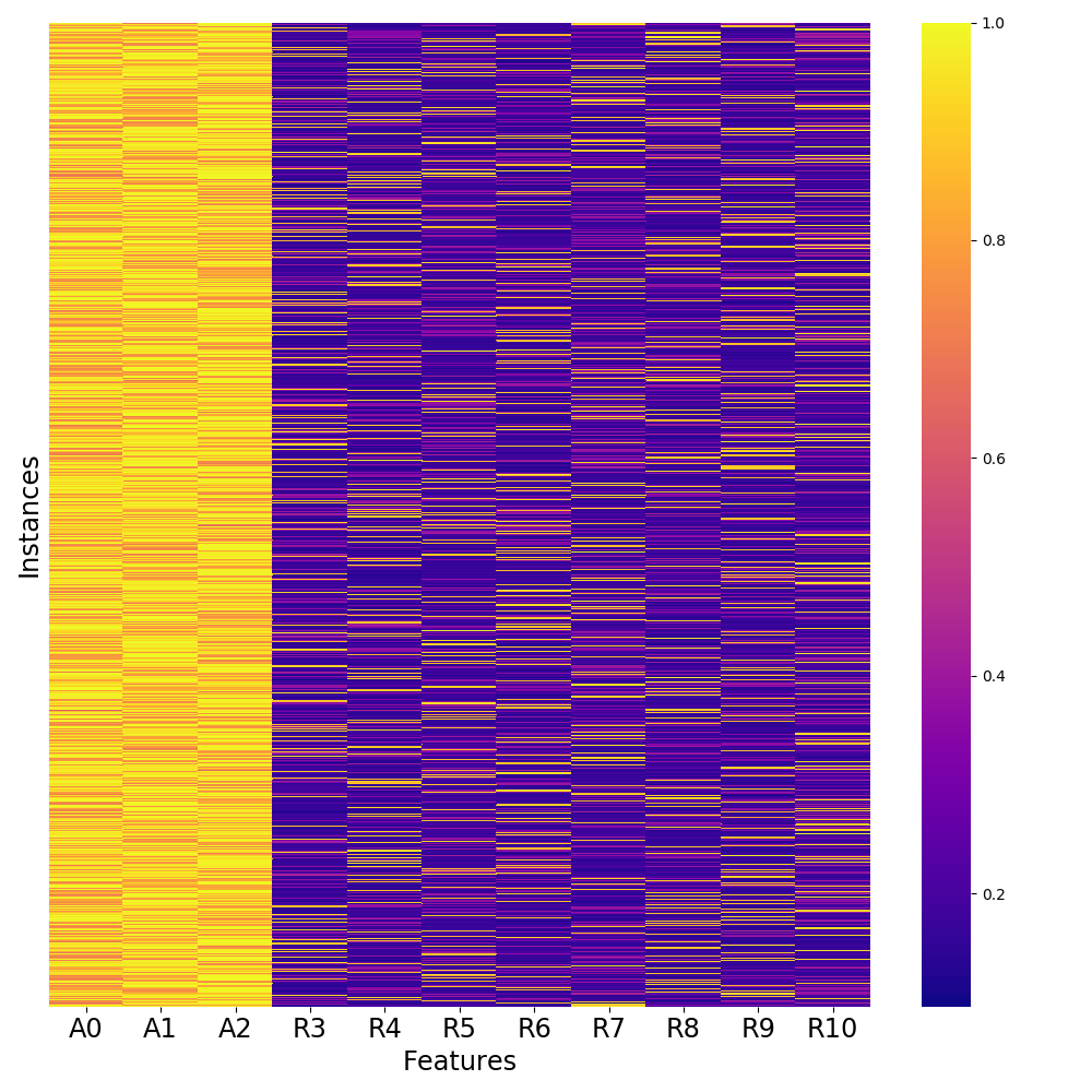
The fourth step seeks to identify the smallest clusters of instances that can be considered significant, i.e. how far down the dendrogram we can travel before the distance between individual clusters are no longer statistically significant ($<0.05$). This will yield some maximum number of significant clusters (k) that can quite likely be larger than the optimal number of meaningful clusters. For example, LCS-DIVE found a maximum of 52 significant clusters for the 11-bit MUX, when the optimal number of clusters is 8. To determine statistically significant clusters we implemented a previously proposed Monte Carlo based method [10]. See Sup.1.3.2 for details on this approach and cluster outputs generated by LCS-DIVE.

The fifth step produces clustermaps for all possible significant cluster counts, i.e from 1 homogeneous cluster (encompassing all instances) to k maximum significant clusters. These can be viewed as distinct clustering hypotheses in search of the optimum. Generating candidate clustermaps from k to 1 is achieved by moving up the dendrogram: merging the closest pair of clusters (i.e. the shortest Ward distance) that also share the same direct parent cluster. This is repeated step-wise until k clustermaps have been generated. Each clustermap can include up to two additional columns: (1) cluster membership labels for each instance and (2) the true underlying cluster membership for each instance, if known and provided by the user, for downstream comparison. Figure 3A gives the significant clustermap (k $=8$) for the 11-bit MUX including columns for the ’found’ clusters, and ’true’ underlying clusters. We can see in this example that the found clusters perfectly align with the true ones. For each clustermap, LCS-DIVE also exports (1) the original dataset, adding a ’clusterID’ column such that followup analyses may be conducted linking instances in the data to identified clusters, and (2) a spreadsheet summarizing cluster analysis characteristics such as ‘within-cluster’ testing accuracy.

The last step seeks to facilitate determination of the ‘optimal’ number of homogeneous clusters. LCS-DIVE employs the elbow method with the distortion metric (i.e. the sum of square distances from each point in a cluster to it’s centroid) [24]. The elbow approach seeks to pick some minimal number of clusters which also minimizes distortion. One elbow plot is generated describing the set of k possible significant clustermaps. Importantly, LCS-DIVE makes all k clustermaps available so that investigators have the option to use their own strategy or judgement for selecting the optimal number of clusters or to compare different candidate heterogeneous subgroup clusters downstream. Figure 3B gives the elbow plot generated for the 11-bit MUX. LCS-DIVE attempts to automatically identify the elbow (i.e optimal cluster count) by rotating the elbow plot counterclockwise about the origin such that the left and right-most points on the curve are level on the y-axis. The selected elbow is the point with the lowest y coordinate. For the 11-bit MUX this approach correctly identifies the optimal 8 instance clusters as seen in Figure 3B. However this strategy is not guaranteed to be optimal in all scenarios.

The third phase of LCS-DIVE differently focuses on clustering and visualizing the set of LCS rules constituting the trained model directly. The goal is to interrogate global feature patterns found across the rules of the model to identify important features and infer underlying patterns of association. This phase formalizes and automates the global rule visualization pipeline first proposed in [34]. First, we take the n trained rule populations and merge them into a single set. This merged rule set is not meant to be applied as a predictive model (due to risk of overfitting) without validation of its performance outside of the original dataset. The second step prepares the rule set for visualization by encoding them based on what features were specified vs. ignored (i.e. generalized) within each rule. Rule encoding is detailed Sup.1.4.

The subsequent steps mirror those from phase two including hierarchical clustering, identification of k significant clusters, generation of heatmaps, and suggested cluster number determination. Figure 4 gives the results of clustering the rule set trained on the 11-bit MUX, with and without post-training rule compaction (using CRA2 [4]). There are no ‘true’ clusters here since we are clustering rules rather than instances. Note that with rule compaction a much cleaner set of rule patterns emerge similar to those observed in Figure 3 using FT scores. Further, a cluster number closer to the ideal 8 feature combination clusters is recommended by the elbow plot approach. Rule compaction has no impact on FT scores that are generated during model training, thus it is not applied in subsequent analyses of this paper. However, it is an important element for improving LCS rule population interpretation as illustrated here [26, 12].

The final phase of LCS-DIVE also operates on the merged rule set, generating a network visualization. The goal here is to further characterize underlying associations by visualizing univariate, epistatic, and heterogeneous patterns captured in the rule set [34]. First, we sum pairwise specified feature co-occurences across the merged binary encoded rule set. Co-specification in rules indicates potential feature interactions [34]. Then a network visualization is generated where nodes are dataset features and node diameter is proportional that features specification across all rules. Edge thickness between nodes represents pairwise co-specification counts of those features across all rules. Figure 5 gives the network generated for the 11-bit MUX with and without CRA2 rule compaction. A clear interaction between the three address bits is seen, and respective (less frequent) heterogeneous interactions between address and respective register bits is also observed. Notice that co-occurences between register bits are negligible (made clearer following rule compaction), offering support in properly characterizing the underlying epistatic and heterogeneous associations underlying the 11-bit MUX.

Here we examine clean and noisy GAMETES datasets D1-D6 with either a univariate, 2-feature additive, or 4-feature additive association. FT clustermaps for each of the 6 datasets are given in Figure 7. As no heterogeneity is simulated here, no ‘true’ subgroups are identified.

For D1 (Figure 7A), a strong signature for the single predictive feature is observed for all instances. Notably the ’found’ clusters are incorrectly picking up on subtle FT signatures in some of the non-predictive features, causing more than one ’optimal’ cluster to be identified. An example of Phase 3 rule population visualizations for D1 is available in Sup.3.2.1. For D2, (Figure 7B) there is a similar univariate signature however a proportion of instances in lower clusters yield a messy signature. These correspond to noisy instances that didn’t follow the modeled univariate pattern. We know from this controlled simulation that these lower clusters are not representative of underlying heterogeneity. LCS-DIVE automatically exports testing accuracy for the instances within respective clusters. From this we confirm that testing accuracy is very high in the top two clusters (capturing the univariate association) but close to zero in the lower ‘noisy’ clusters. Later, this observation will allow us to differentiate between clusters that represent candidate heterogeneous subgroups, and clusters that only capture underlying noise.

For D3 (Figure 7C), we observe a largely strong signature for both features. Notably, this signature is less sharp compared to D1 because: either or both of the predictive features can be applied within a given instance to correctly predict class, but both are not required. This yields LCS rules that specify just one or both features, impacting the resulting FT signature. For D4, (Figure 7D), we can observe 4 unique clusters, i.e. two clusters where only one feature is predictive (because there is noise in the other), a cluster where both features are predictive on their own, and a small cluster at the bottom corresponding to completely noisy instances.

Similarly, for D5 (Figure 7E) we observe the strongest signature for the 4 additive predictive features together, however for D6 (Figure 7F) we observe one larger cluster of instances where all of the features appear predictive, and a number of smaller clusters capturing instances where some subset of the four features was predictive but one or more of the four was not. This pattern of clustering defines a unique signature for additive univariate effects in the context of FT clustering that other patterns of association do not display (shown below).

Here we examine clean and noisy GAMETES datasets D7-D14 examining scenarios of pure epistasis and additive epistasis combinations (i.e. impure epistasis [36]). FT clustermaps for pure epistasis datasets are given in Figure 8 and those for impure epistasis are given in Figure 9.

For D7 (Figure 8A), we observe a strong signature for both interacting predictive features across all instances. Note the subtle difference between this and 2 clean additively combined features from Figure 7C. For D8 (Figure 8B), we observe a strong but less consistent signature for the 2 interacting features. Distinct from the noisy 2-feature additive example (Figure 7D), we don’t see instance clusters where either feature has a strong signature on it’s own. Since this distinction is subtle, we recommend users conduct explicit statistical tests confirming the presence of epistasis vs. additive effects in practice. Similarly, for D9 (Figure 8C), we observe a strong signature for the three interacting predictive features across all instances. For D10 (Figure 8D), we observe a reasonably strong but less consistent signature for the 3 interacting features. However we do not see the same ‘blocky’ signature observed in noisy additive data (Figure 7F) where some features are predictive but not all.

Next we examine impure epistasis scenarios in which features M2P3 and M2P4 are epistatically interacting, and M0P1 and M1P2 are univariate. For D11 (Figure 9A) we observe a much stronger signature for the two univariate features and a much weaker one for the epistatic features. We believe this is because, LCS rule discovery is pressured to find the simplest rules possible (i.e. those that specify the fewest features). Given that accurate predictions can be obtained from either univariate feature alone, it is not surprising that the signature of the interacting features is much weaker. For D12 (Figure 9B), we observe signatures reminiscent of additive univariate associations (i.e. instance clusters where one univariate feature has low scores) as well as epistatic interactions (i.e. where both interacting features have a very strong signature in specific clusters). For D13 (Figure 9C), we observe a largely strong cluster where all four features are consistently high but but neither epistatic pair has as strong a signal as in the 2-way pure epistasis (Figure 8A). Further we observe two small instance clusters where only one of the to pairs has a particularly strong signal. We believe this to be an artifact of rule-based learning where the instances of one epistatic pair constitutes a rarer genotype combination than the other and thus cumulatively receive lower FT updates than the more common pair. For D14 (Figure 9D), we observe a similar, but more drawn out pattern than in D13 as a reflection of the underlying noise.

Here we examine clean and noisy GAMETES datasets D15-D21 examining scenarios with heterogeneous associations. FT clustermaps for heterogeneous combinations of associations are given in Figure 10. Now that we are simulating underlying heterogeneous subgroups, these figures now include both the ’found’ and ’true’ clusters for reference. The number of found clusters presented in each plot is based on the automated recommendation.

For D15 (Figure 10A), with 2 univariate associations combined heterogeneously, we observe three ‘found’ clusters with strong unique signatures. Specifically, two of the clusters emphasize one of the two heterogeneous features and the third has both emphasized. Notice that the upper two found clusters completely overlap with underlying true clusters but the third found cluster is a mix of instances from either underlying model. This is an expected characteristic based on how heterogeneity is simulated with GAMETES. Specifically, instances are generated separately for each underlying model, then the instances are combined into a single dataset. Instances in the top cluster were generated with M0P1 being predictive, and the randomly generated feature value for M1P2 was not predictive in-line with the M1P2 model used to generate the other half of the data. Instances in the middle cluster followed the same pattern but with M0P1 and M1P2 switched. Lastly, in the lowest found cluster where both features were important, the instance feature values happened to correspond to correct classifications based on both the M0P1 and M1P2 models. This yields a signature for the third cluster that is more similar to an epistatic interaction. However this unique ‘overlapping’ form of heterogeneity is characterized by the three distinct clusters. For D16 (Figure 10B), we observe a very similar signature but with an additional cluster of noisy instances (second cluster from the top) which we confirm as noise by examining it’s underlying cluster testing accuracy.

For D17 (Figure 10C), with 4 univariate associations combined heterogeneously, we now observe 5 dominant ‘found’ clusters, i.e. one where all 4 predictive features are important, and four others where only a single one is. The explanation for this expected finding is the same as for D15. For D18, (Figure 10D) we observe the impact of 60$\%$ noise in combination with this ‘overlapping’ form of heterogeneity on the clarity of the FT signature. The lack of a larger cluster where all predictive features have a high FT signature distinguishes it from D6 (i.e. noisy 4-feature additive). While LCS-DIVE has failed to clearly cluster the true underlying subgroups in this scenario, FT clearly distinguishes which features are relevant (i.e. predictive) from those that are not as in all other GAMETES analysis.

For D19 (Figure 10E), we now consider both epistasis and heterogeneity simultaneously. Here we observe 3 dominant ‘found’ clusters, i.e. where one 2-way epistatic interaction, the other, or both are important. This signature is consistent with what we observed for other clean GAMETES heterogeneity simulations, i.e. D15 and D17, but now also capturing underlying epistatic interactions relevant in distinct instance subsets. The extra ‘found’ cluster are a reflection of the simulated model overlap as well as the model only reaching about 76 $\%$ testing accuracy within the allotted training iterations. For D20 (Figure 10F), we observe the same, albeit messier, FT signature in comparison to D19, with three dominant ‘found’ clusters. Again we confirm smaller clusters capture instances that were poorly predicted yielding a less consistent signature. Lastly, for D21 (see Figure 3 of Sup.3.4) we examine the FT signature when an unbalanced proportion of instances (i.e. 75:25) correspond with each of the heterogeneous epistatic models. In this scenario, the more frequent instance subgroup (i.e. 75$\%$) yields a clear 2-way interaction signature, while the second subgroup more ambiguously indicates the involvement of the two additional predictive features. This supports our finding that FT score signatures reliably identify key relevant features in the LCS model, and suggests that this approach will facilitate the characterization of dominant patterns of association while sometimes at the expense of clearly identifying a less frequent heterogeneous association.

Looking across D1-D21 GAMETES simulation results, we found evidence that FT clustermap signatures are generally capable of distinguishing clean and noisy associations that are univariate, additive, epistatic, heterogeneous, and mixed. Further, interrogation of the testing accuracy within ‘found’ clusters helps to discriminate heterogeneous subgroups from ignorable ‘noisy’ clusters and thus guide the selection of the optimal number of clusters for downstream investigation. Another item to pay attention to is the testing accuracy of the LCS model as a whole. FT signature interpretation clearly relies on acknowledgment of how much signal was captured by the model, i.e. FT signatures uniquely vary in clean vs. noisy scenarios. Notably, the FT signatures of scenarios involving additive vs. heterogeneous signatures were similar enough to warrant further discussion and direct comparison. These include (D6 vs. D18) and (D14 vs.D20) as detailed in Sup.3.5. Also note that the overlapping simulation of heterogeneity (simulated by GAMETES) makes such associations more difficult to clearly characterize in contrast with MUX heterogeneity. Real world problems could exhibit heterogeneous associations of either type so we should be prepared to characterize them both. LCS-DIVE run time reports for all phases and datasets are given in Sup.3.6.

References

- [1] E. Bernadó-Mansilla and J. M. Garrell-Guiu. Accuracy-based learning classifier systems: models, analysis and applications to classification tasks. Evolutionary Computation, 11(3):209–238, 2003.
- [2] D. V. Carvalho, E. M. Pereira, and J. S. Cardoso. Machine learning interpretability: A survey on methods and metrics. Electronics, 8(8):832, 2019.
- [3] A. Dahl and N. Zaitlen. Genetic influences on disease subtypes. Annual Review of Genomics and Human Genetics, 21:413–435, 2020.
- [4] P. W. Dixon, D. W. Corne, and M. J. Oates. A ruleset reduction algorithm for the xcs learning classifier system. In P. L. Lanzi, W. Stolzmann, and S. W. Wilson, editors, Learning Classifier Systems, pages 20–29, Berlin, Heidelberg, 2003. Springer Berlin Heidelberg.
- [5] R. ElShawi, Y. Sherif, M. Al-Mallah, and S. Sakr. Interpretability in healthcare: A comparative study of local machine learning interpretability techniques. Computational Intelligence, 2020.
- [6] V. A. Huynh-Thu, Y. Saeys, L. Wehenkel, and P. Geurts. Statistical interpretation of machine learning-based feature importance scores for biomarker discovery. Bioinformatics, 28(13):1766–1774, 2012.
- [7] M. Iqbal, W. N. Browne, and M. Zhang. Xcsr with computed continuous action. In Australasian Joint Conference on Artificial Intelligence, pages 350–361. Springer, 2012.
- [8] M. I. Jordan and T. M. Mitchell. Machine learning: Trends, perspectives, and prospects. Science, 349(6245):255–260, 2015.
- [9] M. Kaushik and B. Mathur. Comparative study of k-means and hierarchical clustering techniques. International Journal of Software & Hardware Research in Engineering, 2(6), 2014.
- [10] P. K. Kimes, Y. Liu, D. Neil Hayes, and J. S. Marron. Statistical significance for hierarchical clustering. Biometrics, 73(3):811–821, 2017.
- [11] P. L. Lanzi, M. V. Butz, and D. E. Goldberg. Empirical analysis of generalization and learning in xcs with gradient descent. In Proceedings of the 9th annual conference on Genetic and evolutionary computation, pages 1814–1821, 2007.
- [12] Y. Liu, W. N. Browne, and B. Xue. Absumption to complement subsumption in learning classifier systems. In Proceedings of the Genetic and Evolutionary Computation Conference, pages 410–418, 2019.
- [13] Y. Liu, W. N. Browne, and B. Xue. Visualizations for rule-based machine learning. Natural Computing, pages 1–22, 2021.
- [14] B. Mirza, W. Wang, J. Wang, H. Choi, N. C. Chung, and P. Ping. Machine learning and integrative analysis of biomedical big data. Genes, 10(2):87, 2019.
- [15] J. H. Moore and B. C. White. Tuning relieff for genome-wide genetic analysis. In European Conference on Evolutionary Computation, Machine Learning and Data Mining in Bioinformatics, pages 166–175. Springer, 2007.
- [16] J. H. Moore and S. M. Williams. Epistasis. Springer, 2016.
- [17] A. A. Motsinger-Reif, S. Deodhar, S. J. Winham, and N. E. Hardison. Grammatical evolution decision trees for detecting gene-gene interactions. BioData mining, 3(1):8, 2010.
- [18] M. M. Najafabadi, F. Villanustre, T. M. Khoshgoftaar, N. Seliya, R. Wald, and E. Muharemagic. Deep learning applications and challenges in big data analytics. Journal of Big Data, 2(1):1, 2015.
- [19] G. Plumb, D. Molitor, and A. S. Talwalkar. Model agnostic supervised local explanations. Advances in Neural Information Processing Systems, 31:2515–2524, 2018.
- [20] P. C. Prorok, G. L. Andriole, R. S. Bresalier, S. S. Buys, D. Chia, E. D. Crawford, R. Fogel, E. P. Gelmann, F. Gilbert, M. A. Hasson, et al. Design of the prostate, lung, colorectal and ovarian (plco) cancer screening trial. Controlled clinical trials, 21(6):273S–309S, 2000.
- [21] Y. Qi. Random forest for bioinformatics. In Ensemble machine learning, pages 307–323. Springer, 2012.
- [22] M. T. Ribeiro, S. Singh, and C. Guestrin. " why should i trust you?" explaining the predictions of any classifier. In Proceedings of the 22nd ACM SIGKDD international conference on knowledge discovery and data mining, pages 1135–1144, 2016.
- [23] M. D. Ritchie, L. W. Hahn, and J. H. Moore. Power of multifactor dimensionality reduction for detecting gene-gene interactions in the presence of genotyping error, missing data, phenocopy, and genetic heterogeneity. Genetic Epidemiology: The Official Publication of the International Genetic Epidemiology Society, 24(2):150–157, 2003.
- [24] E. Rohman and B. Satoto. Integration k-means clustering method and elbow method for identification of the best customer profile cluster. IOP Conference Series: Materials Science and Engineering, 336, 2018.
- [25] A. F. Subar, D. Midthune, M. Kulldorff, C. C. Brown, F. E. Thompson, V. Kipnis, and A. Schatzkin. Evaluation of alternative approaches to assign nutrient values to food groups in food frequency questionnaires. American journal of epidemiology, 152(3):279–286, 2000.
- [26] J. Tan, J. Moore, and R. Urbanowicz. Rapid rule compaction strategies for global knowledge discovery in a supervised learning classifier system. In Artificial Life Conference Proceedings 13, pages 110–117. MIT Press, 2013.
- [27] T. A. Thornton-Wells, J. H. Moore, and J. L. Haines. Dissecting trait heterogeneity: a comparison of three clustering methods applied to genotypic data. BMC bioinformatics, 7(1):204, 2006.
- [28] A. W. Toga, I. Foster, C. Kesselman, R. Madduri, K. Chard, E. W. Deutsch, N. D. Price, G. Glusman, B. D. Heavner, I. D. Dinov, et al. Big biomedical data as the key resource for discovery science. Journal of the American Medical Informatics Association, 22(6):1126–1131, 2015.
- [29] R. Urbanowicz, A. Granizo-Mackenzie, and J. Moore. Instance-linked attribute tracking and feedback for michigan-style supervised learning classifier systems. In Proceedings of the 14th annual conference on Genetic and evolutionary computation, pages 927–934, 2012.
- [30] R. Urbanowicz, N. Ramanand, and J. Moore. Continuous endpoint data mining with exstracs: A supervised learning classifier system. In Proceedings of the Companion Publication of the 2015 Annual Conference on Genetic and Evolutionary Computation, pages 1029–1036, 2015.
- [31] R. J. Urbanowicz, A. S. Andrew, M. R. Karagas, and J. H. Moore. Role of genetic heterogeneity and epistasis in bladder cancer susceptibility and outcome: a learning classifier system approach. Journal of the American Medical Informatics Association, 20(4):603–612, 2013.
- [32] R. J. Urbanowicz, G. Bertasius, and J. H. Moore. An extended michigan-style learning classifier system for flexible supervised learning, classification, and data mining. In International Conference on Parallel Problem Solving from Nature, pages 211–221. Springer, 2014.
- [33] R. J. Urbanowicz and W. N. Browne. Introduction to learning classifier systems. Springer, 2017.
- [34] R. J. Urbanowicz, A. Granizo-Mackenzie, and J. H. Moore. An analysis pipeline with statistical and visualization-guided knowledge discovery for michigan-style learning classifier systems. IEEE computational intelligence magazine, 7(4):35–45, 2012.
- [35] R. J. Urbanowicz, D. Granizo-Mackenzie, and J. H. Moore. Using expert knowledge to guide covering and mutation in a michigan style learning classifier system to detect epistasis and heterogeneity. In International Conference on Parallel Problem Solving from Nature, pages 266–275. Springer, 2012.
- [36] R. J. Urbanowicz, J. Kiralis, N. A. Sinnott-Armstrong, T. Heberling, J. M. Fisher, and J. H. Moore. Gametes: a fast, direct algorithm for generating pure, strict, epistatic models with random architectures. BioData mining, 5(1):1–14, 2012.
- [37] R. J. Urbanowicz, C. Lo, J. H. Holmes, and J. H. Moore. Attribute tracking: strategies towards improved detection and characterization of complex associations. In Proceedings of the Genetic and Evolutionary Computation Conference, pages 553–560, 2018.
- [38] R. J. Urbanowicz and J. H. Moore. Learning classifier systems: a complete introduction, review, and roadmap. Journal of Artificial Evolution and Applications, 2009, 2009.
- [39] R. J. Urbanowicz and J. H. Moore. The application of michigan-style learning classifier systems to address genetic heterogeneity and epistasis in association studies. In Proceedings of the 12th annual conference on Genetic and evolutionary computation, pages 195–202, 2010.
- [40] R. J. Urbanowicz and J. H. Moore. Exstracs 2.0: description and evaluation of a scalable learning classifier system. Evolutionary intelligence, 8(2-3):89–116, 2015.
- [41] R. J. Urbanowicz, R. S. Olson, P. Schmitt, M. Meeker, and J. H. Moore. Benchmarking relief-based feature selection methods for bioinformatics data mining. Journal of biomedical informatics, 85:168–188, 2018.
- [42] R. J. Urbanowicz and R. Zhang. Lcs dive software. url=https://github.com/UrbsLab/LCS-Visualization-Pipeline, March 2021.
- [43] R. J. Urbanowicz and R. Zhang. scikit-exstracs software. url=https://github.com/UrbsLab/scikit-ExSTraCS, March 2021.
- [44] M. Waskom and the seaborn development team. seaborn. url=https://github.com/mwaskom/seaborn, March 2021.
- [45] S. W. Wilson. Classifier systems and the animat problem. Machine learning, 2(3):199–228, 1987.
- [46] S. W. Wilson. Classifier fitness based on accuracy. Evolutionary computation, 3(2):149–175, 1995.
- [47] R. F. Zhang and R. J. Urbanowicz. A scikit-learn compatible learning classifier system. In Proceedings of the 2020 Genetic and Evolutionary Computation Conference Companion, pages 1816–1823, 2020.