Image Modeling with
Deep Convolutional Gaussian Mixture Models
Abstract
In this conceptual work, we present Deep Convolutional Gaussian Mixture Models (DCGMMs): a new formulation of deep hierarchical Gaussian Mixture Models (GMMs) that is particularly suitable for describing and generating images. Vanilla (i.e., flat) GMMs require a very large number of components to describe images well, leading to long training times and memory issues. DCGMMs avoid this by a stacked architecture of multiple GMM layers, linked by convolution and pooling operations. This allows to exploit the compositionality of images in a similar way as deep CNNs do. DCGMMs can be trained end-to-end by Stochastic Gradient Descent. This sets them apart from vanilla GMMs which are trained by Expectation-Maximization, requiring a prior k-means initialization which is infeasible in a layered structure. For generating sharp images with DCGMMs, we introduce a new gradient-based technique for sampling through non-invertible operations like convolution and pooling. Based on the MNIST and FashionMNIST datasets, we validate the DCGMMs model by demonstrating its superiority over flat GMMs for clustering, sampling and outlier detection.
Index Terms:
Deep Learning, Gaussian Mixture Models, Deep Learning, Deep Convolutional Gaussian Mixture Models, Stochastic Gradient DescentI Introduction
This conceptual work is in the context of probabilistic image modeling, whose main objectives are both, density estimation and image generation (sampling). Since images usually do not precisely follow a Gaussian mixture distribution, such a treatment is inherently approximative in nature. Image generation is currently a very active research topic, and similar techniques are being investigated for generating videos [9, 25].
An issue with many recent approaches is the lack of density estimation capacity, i.e., explicitly expressing the learned probability-under-the-model of an image .
In contrast, GMMs explicitly describe the distribution , given by a set of training data , as a weighted mixture of Gaussian component densities :
| (1) |
Conceptually, GMMs are latent-variable models: it is assumed that the unobservable (latent) variable determines from which component a data vector has been sampled, which is expressed as
| (2) |
Marginalizing the latent variable in eq. 2, we obtain eq. 1.
GMMs require the mixture weights to be normalized: and the covariance matrices to be positive definite: . The quality of the current fit-to-data is expressed by the (incomplete) log-likelihood
| (3) |
which is what GMM training optimizes, usually by variants of Expectation-Maximization (EM) [4]. It is shown that any distributions can be approximated by mixtures of Gaussians given enough components [11]. Thus, GMMs are guaranteed to model the complete data distribution, but only to the extent allowed by the number of components .
In this respect, GMMs are similar to flat neural networks with a single hidden layer. Although, by the universal approximation theorem of [26] and [14], they can approximate arbitrary functions (from certain rather broad function classes), they fail to do so in practice. The reason for this is that the number of required hidden layer elements is unknown, and usually beyond the reach of any reasonable computational capacity. For images, this problem was largely solved by introducing deep Convolutional Neural Networks (CNNs). CNNs model the statistical structure of images (hierarchical organization and translation invariance) by chaining multiple convolution and pooling layers. Thus, the number of parameters can be reduced without compromising accuracy.
I-A Objective, Contribution and Novelty
The objective of this article is to introduce a GMM architecture which exploits the same principles that led to the performance explosion of CNNs. In particular, the genuinely novel characteristics are:
- •
conceptually new formulation of deep GMMs, including convolution and pooling operations
- •
scalable end-to-end training by SGD from random initial conditions (no k-means initialization)
- •
efficient large-scale training on high-demensional images
- •
realistic sampling despite non-invertible operations (pooling, convolutions)
- •
better empirical performance than vanilla GMMs on images for sampling, clustering and outlier detection
In addition, we provide a publicly TensorFlow implementation which supports a Keras-like construction of DCGMMs.
I-B Related Work
GANs and VAEs The currently most widely used models of image modeling and generation are Generative Adverserial Networks (GANs) [1, 22, 12] and Variational AutoEncoders (VAEs). GANs are capable of sampling photo-realistic images [28], but are unable to perform density estimation since there is no way to obtain for a given sample . Furthermore, their probabilistic interpretation remains unclear since they do not possess a differentiable loss function that is minimized by training. They may suffer from what is termed mode collapse, which is hard to detect automatically due to the absence of a loss function [28]. VAEs show similar performance when it comes to sampling, in addition to minimizing a differentiable loss function. Moreover, density estimation with VAEs is problematic. Similar approaches, with similar strengths in sampling but a lack of density estimation, are realized by the PixelCNN architecture[23], GLOW[18] and their variants.
Hierarchical GMMs A hierarchical extension of GMMs is presented by [20] with the goal of unsupervised clustering: responsibilities of one GMM are treated as inputs to a subsequent GMM, together with an adaptive mechanism that determines the depth of the hierarchy. [6] present a comparable, more information-theoretic approach but not targetting sampling either. The closest related work to the model we present here is described in [32, 31, 30]. All of these models perceive hierarchical GMMs as modular decompositions of GMMs that are flat. The conceptual foundation is that sampling from a GMM implies the transformation of a normally distributed latent variable by a single GMM component , with weight , as . This leads to a distribution . The choice which GMM component is allowed to transform the latent variable is based on component weights . Hierarchical GMMs are now realized by several sampling steps (layers), and the sampling results of the previous layer representing the latent variable to be transformed by the next one. None of these models consider convolutional or max-pooling operations which have been proven to be important for modeling the statistical structure of images.
Mixture of Factor Analyzers (MFAs) MFAs models [21, 8] can be considered as hierarchical GMMs because they are formulated in terms of a lower-dimensional latent-variable representation, which is mapped to a higher-dimensional space. The use of MFAs for describing natural images is discussed in detail in [28], showing that the MFA model alone, without further hierarchical structure, compares quite favorably to GANs when considering image generation.
Hierarchical Mixture Models An interesting overview of the current research landscape in terms of hierarchical generative mixture models is given in [16]. All of these models are, in principle, capable of sampling and density estimation although the quality of sampling, and the data they can be trained on, vary considerably. Principal competitors in this domain are Sum-Product Networks (SPNs, see, e.g., [27]), which are tree structures of arbitrary depth, with leaves that represent tractable distribution families (typically multi-variate normal, binomial or student-t distributions). SPN nodes perform either weighted summation or multiplication, and with appropriate constraints on the tree structure it can be shown that sampling, inference and density estimation remain tractable. Problems include finding a suitable SPN structure, and dealing with complex and high-dimensional data. Convolutional extensions of the SPN model exist, although they have been applied to very small images only [2]. A similar approach is represented by probabilistic circuits (PCs, see, e.g., [24]) or Tensorial Mixture Models (TMMs, see, e.g., [29]).
Convolutional GMMs The only work we could identify proposing hierarchical convolutional GMMs is [10]. This work describes a hybrid model combining a CNN and a GMM.
SGD and End-To-End Training for GMMs Training GMMs by Stochastic Gradient Descent (SGD) is challenging due to local optima and the need to enforce model constraints, most notably the constraint of positive-definite covariance matrices. At the same time, SGD is attractive in deep architectures due to its simplicity, which is facilitated even further by modern machine learning packages that perform automatic differentiation. SGD for GMMs has recently been discussed in [15], although the proposed solution requires parameter initialization by k-means and introduces several new hyper-parameters. Thus, it is unlikely to work as-is in a hierarchical structure. An SGD approach that achieves robust convergence even without k-means-based parameter initialization is presented by [7]. Undesirable local optima caused by random parameter initialization are circumvented by an adaptive annealing strategy. SPNs and PCs can be trained end-to-end by SGD as well, although no article describes this in detail. It is presumable that data-driven initialization is required, as well. Previous hierarchical GMM proposals [32, 31, 30] use (quite complex) extensions of the EM algorithm initialized by k-means for training. In [28], training is performed using SGD, although with a k-means initialization.
II DCGMM: Model Overview
The Deep Convolutional Gaussian Mixture Model (DCGMM) is a hierarchical model consisting of layers in analogy to CNNs.11 1 Repository: https://gitlab.cs.hs-fulda.de/ML-Projects/dcgmm Each layer with index expects an input tensor of the dimensions and produces an output tensor of dimensions the . Layers can have internal variables that are adapted during SGD training.
A DCGMM layer has two basic operating modes (see fig. 1): for (density) estimation, an input tensor from layer is transformed into an output tensor . For sampling, the direction is reversed: each layer receives a control signal from layer (same dimensions as ), which is transformed into a control signal to layer (same dimensions as ).

II-A Layer Types
We define four layer types: Folding (F), Pooling (P), Linear Classifier (C) and GMM (G). Each implements distinct operations for both modes, i.e., estimation and sampling.
II-A1 Folding Layer
For density estimation, this layer performs a part of the convolution operation well-known from CNNs. Based on the filter sizes , and the filter strides , , all entries of the input tensor inside the range of the sliding filter window are dumped into the channel dimension of the output tensor. We thus obtain an output tensor of dimensions , and , whose entries are computed as with , and . When sampling, the inverse mapping is performed which is not a one-to-one correspondence: input tensor elements which receive several contributions are averaged over all these.
II-A2 Pooling Layer
For density estimation, pooling layers perform the same operations as standard (max-)pooling layers in CNNs based on the kernel sizes , and strides , . When sampling, pooling layers perform a simple nearest-neighbor up-sampling by a factor indicated by the kernel sizes and strides.
II-A3 GMM Layer
This layer type contains GMM components, each of which is associated with trainable parameters , and , , representing the GMM weights, centroids and covariances. What makes GMM layers convolutional is that they do not model single input vectors, but the channel content at all positions of the input , using a shared set of parameters. This is analogue to the way a CNN layer models image content at all sliding window positions using the same filters. A GMM layer maps the input tensor to , each GMM component contributing the likelihood of having generated the channel content at position (for sample in the mini-batch). This likelihood is often referred to as responsibility and is computed as
| (4) |
For training the GMM layer, we optimize the GMM log-likelihood for each layer :
| (5) |
Training is performed by SGD according to the technique, and with the recommended parameters, presented by [7], which uses a max-component approximation to . In sampling mode, a control signal is produced by standard GMM sampling, performed separately for all positions . GMM sampling at position first selects a component by drawing from a multinomial distribution. If the GMM layer is the last layer of a DCGMM instance, the multinomial’s parameters are the mixing weights for each position . Otherwise, the control signal received from layer is used. It is consistent to use the control signal for component selection in layer , since it was sampled by layer , which was in turn trained on the component responsibilities of layer , see section V. The selected component (still at position ) then samples . It is often beneficial for sampling to restrict the selected number to the components with the highest control signal (top- sampling). This reduces the diversity of sampling as fewer components can participate, but improves its quality since selection is restricted to the most likely components.
II-A4 Linear Classifier Layer
This layer type implements a linear classifier, trained in a supervised manner by cross-entropy loss. Logits are obtained via an affine transformation from the flattened input activities . The logits have the dimension , with representing the number of classes or categories. For sampling, a control signal is generated by approximately inversing this transformation: , where contains the one-hot coded classes for each sample to be generated.
II-B Architecture-Level Functionalities
II-B1 End-to-End Training
To train an DCGMM instance, we optimize for each GMM layer by vanilla SGD22 2 Advanced SGD strategies like RMSProp [13] or Adam [17] seem incompatible with GMM optimization., using learning rates . This is different from a standard CNN classifier, where only a single loss function is minimized. Usually a cross-entropy loss is computed from the last layer’s outputs. Learning is not conducted layer-wise but end-to-end. Parameter initialization for GMM layers selects the initial values for the mixing weights as . Centroid elements sampled from and diagonal covariances are initialized to unit entries. Training is conducted in two steps to ensure convergence. First, only centroids are adapted, whereas both centroids and precisions are adapted in the second step.
II-B2 Density Estimation and Outlier Detection
Outlier detection requires the computation of long-term averages in all layers and positions, and variances over the training set, preferably during a later, stable part of training. Thus, for every layer and position , inliers are characterized by
| (6) |
A larger implies a less restrictive identification of inliers.
II-B3 Sampling and Sharpening
Sampling starts in the highest layer , assumed to be an GMM layer, and propagates control signals downwards (see fig. 1 and section II-A3), with control signal constituting the sampling result. Sampling suffers from information loss due to the non-invertible mappings effected by Pooling and Folding layers. To counteract this, a Folding or Pooling layer at performs sharpening on the control signal it generates from . This involves computing for the GMM layer at level and performing gradient ascent steps . The reason for sharpening is that filters in Folding layers usually overlap, and neighboring filter results are correlated. This correlation is captured by all higher GMM layers, and most prominently by the next-highest one. Therefore, modifying by gradient ascent will recover some of the information lost by pooling or folding. After sharpening, the tensor is passed as control signal to .
II-B4 Conditional Sampling
By conditional sampling we understand the ability to selectively produce samples from a certain class. Obviously, this is only possible when the DCGMM instance has a top-level linear classifier layer. We proceed as in section II-B3, except for the component selection in the top-level GMM layer. For conditional sampling, we simply train a linear classifier in the last layer on the outputs of the previous layer, and then approximately invert this mapping given a certain class label to obtain a control signal for sampling in layer .
II-B5 In-Painting
This is a functionality where a corrupted image, from which a part has been deleted, is supplied to a trained DCGMM instance, which then completes the missing parts. Here, we add a twist by not informing the model on which parts of the image have been deleted. Rather, a DCGMM should infer this on its own using its outlier detection capability, see section II-B2.
Mathematically, in-painting requires that we perform posterior inference from a trained DCGMM. We shall consider this kind of inference for a flat GMM first, and subsequently generalize to DCGMMs.
Assuming that an image is composed of two parts and , where is corrupted. To recover it, we wish to draw samples from the distribution . A simple computation yield an expression that can be evaluated by re-introducing the latent variable of the GMM, see eq. 2:
| (7) |
This shows that the distribution we wish to sample from is again a Gaussian mixture. The mixture coefficients are given by the responsibilities , whereas the component densities can be simplified as . We first draw a value from a multi-nomial distribution defined by , and then generate a sample from component probability of the Gaussian mixture. The part of that belongs to is simply limited when sampling.
In a DCGMM, we implement this procedure for every position in all GMM layers. We start at the top of the hierarchy (layer ), where responsibilities are simply the activities computed by forward-propagating the corrupted input in estimation mode. The responsibilities are used to draw for each position as detailed above. Using , we obtain a control signal for layer as
| (8) |
which propagated downwards through pooling and folding layers to the next-deeper GMM layer.
As for each GMM layer , we want to in-paint only those parts which are not corrupted. We combine the raw control signal and the activities obtained in the forward pass into a fused control signal
where outliers are determined as described in section II-B2. Thus, control signals fill in the activities that seem corrupted.
II-B6 Variant Generation
Variant generation is a special case of sampling, where a template image is supplied and the DCGMM generates similar ones. This requires forward-propagating the template image in estimation mode through the DCGMM, and subsequently sampling a control signal from the top-level GMM layer according to the obtained top-level activities . For all layers sampling is performed as detailed in section II-B3. An interesting option is to control the similarity to the template image. This can be done either by selecting a suitable for top--sampling, or by limiting top-down signals to activities in higher DCGMM layers:
| (11) |
where is a free parameter. The closest match between template image and generated image is to be expected for , whereas should result in very diverse results.
III Experiments
| - | - | - | - | - | - | - | ||
| 1 | F(28,28,1,1) | F(20,20,8,8) | F(7,7,7,7) | F(8,8,2,2) | F(28,28,1,1) | F(4,4,2,2) | F(3,3,1,1) | F(28,28,1,1) |
| 2 | G(25) | G(25) | G(25) | G(25) | G(25) | G(25) | G(25) | G(25) |
| 3 | F(2,2,1,1) | F(4,4,1,1) | F(11,11,1,1) | F(1,1,1,1) | F(13,13,1,1) | P(2,2) | F(1,1,1,1) | |
| 4 | G(36) | G(36) | G(36) | G(36) | G(36) | F(4,4,1,1) | G(25) | |
| 5 | G(25) | F(1,1,1,1) | ||||||
| 6 | P(2,2) | G(25) | ||||||
| 7 | F(6,6,1,1) | |||||||
| 8 | G(49) | |||||||
| comment | vanilla | 1 conv. | 1 conv. | 1 conv. | no | 1 conv. | 2 conv. | no |
| GMM | layer | layer | layer | convolutions | layer | layers | convolutions |
We define various DCGMM instances (with 2 or 3 GMM layers) for evaluation, see table I, plus a single-layer DCGMM baseline which is nothing but a vanilla GMM. A DCGMM instance is defined by the parameters of its layers: Folding(, , , ), (Max-)Pooling(, , , ) and GMM(). Unless stated otherwise, training is always conducted for 25 epochs, using the recommended parameters from [7]. Sharpening is always performed for iterations with a step size of .
III-A Datasets
For the evaluation we use the following image datasets:
MNIST [19] is the common benchmark for computer vision systems and classification problems. It consists of gray scale images of handwritten digits (0-9).
FashionMNIST [33] consists of images of clothes in 10 categories and is structured like the MNIST dataset.
Although these datasets are not particularly challenging for classification, their dimensionality of is at least one magnitude higher than datasets in the literature, which are used for validating other hierarchical GMM approaches in the literature.
III-B Sampling, Sparsity and Interpretability

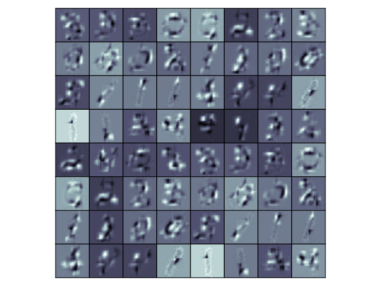
We show that trained DCGMM parameters are sparse and have an intuitive interpretation in terms of sampling. To this effect, we train DCGMM instance - (see table I). After training (see section II-B1), we plot and interpret the centroids of the GMM layers (G2) and (G4). The centroids of layer 2 (left of fig. 2) are easily interpretable and reflect the patterns that can occur in any of the input patches to layer G2 of size . The centroids of G4 (right of fig. 2) express typical responsibility patterns computed from each of the input patches to G2. They are, very sparsely populated. Another interpretation of G4 centroids can be found in terms of sampling (see section II-B3), which would first select a random G4 component to generate a sample of dimensions , and pass it on as a control signal to G2. Traversing Folding layer 3 only reshapes the control signal to dimension , depicted in the middle of fig. 2. This signal controls component selection in each of the positions in G2. Due to their sparsity, we can directly read off the components likely to be selected for sampling at each position. Thus, G2 generates a control signal whose positions of dimensions overlap in the input plane (this is resolved by sharpening in Folding layer 1). In this case, it is easy to see that sampling produces a particular representation of the digit zero.
III-C Outlier Detection
For outlier detection, we compare DCGMM architectures from table I, using the log-likelihood of the highest layer as a criterion as detailed in section II-B2. We first train a DCGMM instance on classes 0-4, and subsequently use the trained classes for inlier- and class 5-9 for outlier-detection. We vary in the range , resulting in different outlier and inlier percentages. fig. 3 shows the ROC-like curves which clearly indicate that the deep convolutional DCGMM instances perform best. However, deep but non-convolutional instances like - and - consistently perform badly.
III-D Clustering
We compare DCGMMs to vanilla GMMs using established clustering metrics, namely the Dunn index [5] and the Davies-Bouldin score [3]. The DCGMM instances from table I are tested on both image datasets. We observe (see table II and fig. 3) that mainly the deep but non-convolutional DCGMM instances perform well in clustering, whereas convolutional instances, even if they are deep, are compromised. These metrics do not measure the classification accuracy obtained by clustering but intrinsic clustering-related properties.
| Dataset | - | - | - | - | - | - | - | ||
| MNIST | Dunn index | 0.14 | 0.14 | 0.13 | 0.12 | 0.19 | 0.15 | 0.15 | |
| DB score | 2.59 | 2.73 | 3.06 | 2.62 | 2.57 | 2.65 | 2.53 | ||
| Fashion- | Dunn index | 0.14 | 0.15 | 0.16 | 0.15 | 0.11 | 0.11 | 0.096 | 0.13 |
| MNIST | DB score | 2.37 | 2.77 | 2.62 | 2.7 | 2.40 | 2.92 | 3.2 | 2.35 |
III-E Sampling and Sharpening
The results presented here were obtained by training on classes 0-4 of both datasets, and have to be confirmed by visual inspection of generated samples. The restriction to classes 0-4 is purely for visualization purposes.
Effects of Convolutional Architectures
An important property of DCGMM is the ability to analyze local input patches. In this experiment, we evaluate sampling for various two-layer architectures with different local patch sizes (i.e., convolution filter): global (-), large (-), semi-local (-) and local (-) and observe effects when performing top-1-sampling. The results of fig. 4 indicate that as filter sizes decrease, the diversity but also the sharpness of generated samples increases at essentially no additional computational cost. Analogous FashionMNIST results are given in fig. 5.


Controlling Diversity by Top-S-Sampling
Using instance -, fig. 5 demonstrates how sample diversity is related to . A higher value yields more diverse samples (see fig. 6), but increases the risk of generating corrupted samples or outliers. As the FashionMNIST results show, a good value of is clearly problem-dependent.


Generating Sharp Images
Figure 7 shows the effect of sharpening for DCGMM instance - using top-1-sampling. We can observe that the overall shape of a sample is not changed but that the outlines are sharper, an effect visible especially for FashionMNIST. Thus, sharpening does no harm and rather improves the visual quality of generated samples.




IV Probabilistic Interpretation of DCGMMs
A probabilistic interpretation of the DCGMM model is possible despite its complex structure. The simple reason is that DCGMM instances produce outputs which are inherently normalizable, meaning that the integral over an infinite domain (e.g., data space) remains finite. Thus, DCGMM outputs can be interpreted as a probability, which is not the case for DNN/CNNs due to the use of scalar products.
Here, we prove that GMMs are normalizable in the sense that the integral of the log-probability is finite. This holds for any GMM layer in a hierarchy regardless of its input, provided that the input is finite (which is assured as Pooling and Folding layers cannot introduce infinities). For simplicity, we integrate over the whole -dimensional space . Since the component probabilities are Gaussian and strictly positive, and therefore the mixing weights are normalized and , the sum is strictly positive. Thus, it is sufficient to show that the integral over the inner sum (argument of the logarithm) is finite. We thus have
| (12) | ||||
which is trivially finite because Gaussians are normalized.
V Conceptual and Practical Differences to Other Hierarchical GMM Models
In this work, we outline the main conceptual differences to what we consider the closest related work, namely the hierarchical GMM models presented in [32, 31, 30]. Besides some differences, they share the notion that a GMM performs sampling by transforming what is termed a random latent variable. This process usually follows a simple distribution like .
To clarify a purely semantic point: In this work, and close to the original derivation of the EM algorithm for GMMs [4], we consider the latent variable of a GMM to be the one that enters into the complete-data log-likelihood of the corresponding latent-variable model. Another point where we differ in terminology is our perception of lower layers being closer to the input in density estimation mode. The lowest layer has index 1, counting upwards.
On the conceptual side, the cited models all share the notion that the proposed deep GMMs have a one-to-one correspondence to a flat model, which is actually the one whose log-likelihood is optimized. Consequently, layers are not optimized independently of each other, but are intrinsically linked. This is most easily visible from the fact that the component weights in each layer are not normalized. Only the aggregated weights of all sampling paths through the deep model have this property.
In contrast, our model does not assume (or require) a one-to-one correspondence to a flat GMM. The layers in our model are GMMs in their own right, having, e.g., their own, normalized weights and losses, and compute the posterior probabilities of their own latent variables. The dependency between layers is realized simply by the fact that posterior probabilities of one GMM layer are inputs to the subsequent GMM layer (potentially after being transformed by convolution and pooling layers).
The first practical consequence of this independent layers type of formulation is that layers can be optimized independently of each other. In particular, it is not necessary to enumerate all possible paths through the deep GMM as in [31] for training, which can only be approximated. Normal GMM optimization is rather performed for each layer, given the outputs of previous layers. This leads to a huge gain in scalability and allows deep GMMs with many layers to be trained on high-dimensional data, such as images, in a matter of minutes.
Another consequence concerns the introduction of pooling and convolution operations: since the layers of our model are not constrained by a joint flat GMM assumption, we are free to apply arbitrary transformations to their outputs before passing these on to subsequent GMM layers. The probabilistic interpretation of our model comes from the fact that each GMM in the model is independent and has the probabilistic interpretation that all GMMs share.
A last consequence concerns sampling. In our formulation of deep GMMs, a single GMM layer is trained on (estimated) latent variables from a preceding layer. When sampling, it can generate a valid instance of these latent variables. Therefore, it is reasonable to use the generated for selecting the GMM component to sample from in layer , instead of the . Of course, a suitable merging of both quantities is possible. Sampling, as described here, is a non-linear instead of an affine transformation, which is similar to the modeling related works. Nevertheless, we retain the notion of paths through the DCGMM instance, given by the components selected for sampling in each layer. Due to the fact that the number of paths grows exponentially with the number of layers, deeper DCGMM instances can describe much richer sample distributions.
VI Summary, Discussion and Conclusion
The Objective of the article was to establish the conceptual foundations of deep GMM hierarchies (see also Section IV) that leverage important mechanisms from the CNN domain. Conceptual differences and shared properties w.r.t. principal related works are discussed in V. Convolution and pooling layers make it possible to apply the model to high-dimensional image data with off-the-shelf hardware (typical training runs take approximately minutes on a GeForce GTX 1080).
Results show the illustration of important functionalities such as outlier detection, clustering and sampling, which no other work on hierarchical GMMs can present for such high-dimensional image datasets. We also propose a method to generate sharp images with GMMs, which has been a problem in the past [28]. An interesting facet of our experimental results is that non-convolutional DCGMMs seem to perform better at clustering, whereas convolutional ones are better at outlier detection and sampling.
A Key point is the compositionality in natural images. This property is at the root of DCGMM’s ability to produce realistic samples with relatively few parameters. When considering top-S-sampling in a layer with positions, the number of distinct control signals generated layer is . A DCGMM instance with multiple GMM layers can thus sample different patterns, which grows with the depth of the hierarchy and the number of distinct positions in a layer, making a strong argument in favor of deep convolutional hierarchies such as DCGMM. This is an argument similar to the one about different paths through a hierarchical MFA model in [32, 31]. However, the number of paths grow more strongly for DCGMMs because sampling is performed independently for each GMM position.
Practical advantages over other hierarchical models such as [32, 31, 30] are most notably the introduction of convolution and pooling layers. Our experimental validation can be performed on high-dimensional data, such as images, with moderate computational cost. This contradicts low-dimensional problems such as the artificial Smiley task or the Ecoli and related problems. Our experimental validation does not exclusively focus on clustering performance (problematic with images), but on demonstrating the capacity for realistic sampling and outlier detection. Lastly, training DCGMMs by SGD facilitates efficient parallelizable implementations, as demonstrated by the TF2 implementation provided.
Next steps consist of exploring more DCGMM architectures, mainly sampling, for generating natural images.
References
- [1] Martin Arjovsky, Soumith Chintala, and Léon Bottou. Wasserstein GAN. 2017.
- [2] Cory J Butz, Jhonatan S Oliveira, André E dos Santos, and André L Teixeira. Deep convolutional sum-product networks. In Proceedings of the AAAI Conference on Artificial Intelligence, volume 33, pages 3248–3255, 2019.
- [3] David L. Davies and Donald W. Bouldin. A Cluster Separation Measure. IEEE Transactions on Pattern Analysis and Machine Intelligence, PAMI-1(2):224–227, 1979.
- [4] A. P. Dempster, N. M. Laird, and D. B. Rubin. Maximum Likelihood from Incomplete Data Via the EM Algorithm . Journal of the Royal Statistical Society: Series B (Methodological), 39(1):1–22, 1977.
- [5] J. C. Dunn. A fuzzy relative of the ISODATA process and its use in detecting compact well-separated clusters. Journal of Cybernetics, 3(3):32–57, 1973.
- [6] Vincent Garcia, Frank Nielsen, and Richard Nock. Hierarchical Gaussian mixture model. In 2010 IEEE International Conference on Acoustics, Speech and Signal Processing, pages 4070–4073. IEEE, 2010.
- [7] Alexander Gepperth and Benedikt Pfülb. Gradient-based training of gaussian mixture models in high-dimensional spaces, 2020.
- [8] Zoubin Ghahramani and Geoffrey E. Hinton. The EM Algorithm for Mixtures of Factor Analyzers. Compute, pages 1–8, 1997.
- [9] Farhad Ghazvinian Zanjani, Svitlana Zinger, and Peter H. N. de With. Deep convolutional gaussian mixture model for stain-color normalization of histopathological images. In Alejandro F. Frangi, Julia A. Schnabel, Christos Davatzikos, Carlos Alberola-López, and Gabor Fichtinger, editors, Medical Image Computing and Computer Assisted Intervention – MICCAI 2018, pages 274–282, Cham, 2018. Springer International Publishing.
- [10] Farhad Ghazvinian Zanjani, Svitlana Zinger, and Peter H. N. de With. Deep Convolutional Gaussian Mixture Model for Stain-Color Normalization of Histopathological Images. In Miccai, volume 1, pages 274–282. Springer International Publishing, 2018.
- [11] Ian Goodfellow, Yoshua Bengio, and Aaron Courville. Deep Learning. MIT Press, 2016. http://www.deeplearningbook.org.
- [12] Ian J. Goodfellow, Jean Pouget-Abadie, Mehdi Mirza, Bing Xu, David Warde-Farley, Sherjil Ozair, Aaron Courville, and Yoshua Bengio. Generative adversarial nets. Advances in Neural Information Processing Systems, 3(January):2672–2680, 2014.
- [13] Geoffrey Hinton, Nitish Srivastava, and Kevin Swersky. Lecture 6.5 - RmsProp: Divide the gradient by a running average of its recent magnitude, 2012.
- [14] Kurt Hornik, Maxwell Stinchcombe, and Halbert White. Multilayer feedforward networks are universal approximators. Neural Networks, 2(5):359–366, 1989.
- [15] Reshad Hosseini and Suvrit Sra. An alternative to EM for Gaussian mixture models: batch and stochastic Riemannian optimization. Mathematical Programming, 181(1):187–223, 2020.
- [16] Priyank Jaini, Pascal Poupart, and Yaoliang Yu. Deep homogeneous mixture models: Representation, separation, and approximation. In NeurIPS, pages 7136–7145, 2018.
- [17] Diederik P. Kingma and Jimmy Lei Ba. Adam: A method for stochastic optimization. 3rd International Conference on Learning Representations, ICLR 2015 - Conference Track Proceedings, pages 1–15, 2015.
- [18] Diederik P Kingma and Prafulla Dhariwal. Glow: generative flow with invertible 1 1 convolutions. In Proceedings of the 32nd International Conference on Neural Information Processing Systems, pages 10236–10245, 2018.
- [19] Yann LeCun, Léon Bottou, Yoshua Bengio, and Patrick Haffner. Gradient-based learning applied to document recognition. Proceedings of the IEEE, 86(11):2278–2323, 1998.
- [20] Ming Liu, Eric Chang, and Bei Qian Dai. Hierarchcial Gaussian mixture model for speaker verification. 7th International Conference on Spoken Language Processing, ICSLP 2002, pages 1353–1356, 2002.
- [21] Geoffrey McLachlan and David Peel. Mixtures of Factor Analyzers. pages 238–256, jan 2005.
- [22] Mehdi Mirza and Simon Osindero. Conditional Generative Adversarial Nets. pages 1–7, 2014.
- [23] Aäron van den Oord, Nal Kalchbrenner, Oriol Vinyals, Lasse Espeholt, Alex Graves, and Koray Kavukcuoglu. Conditional Image Generation with PixelCNN Decoders. In Proceedings of the 30th International Conference on Neural Information Processing Systems, NIPS’16, page 4797–4805, Red Hook, NY, USA, 2016. Curran Associates Inc.
- [24] Robert Peharz, Steven Lang, Antonio Vergari, Karl Stelzner, Alejandro Molina, Martin Trapp, Guy Van den Broeck, Kristian Kersting, and Zoubin Ghahramani. Einsum networks: Fast and scalable learning of tractable probabilistic circuits. In International Conference on Machine Learning, pages 7563–7574. PMLR, 2020.
- [25] Aj Piergiovanni and Michael Ryoo. Temporal Gaussian mixture layer for videos. In Kamalika Chaudhuri and Ruslan Salakhutdinov, editors, Proceedings of the 36th International Conference on Machine Learning, volume 97 of Proceedings of Machine Learning Research, pages 5152–5161, Long Beach, California, USA, 09–15 Jun 2019. PMLR.
- [26] Allan Pinkus. Approximation theory of the MLP model in neural networks. Acta Numerica, 8:143–195, 1999.
- [27] Hoifung Poon and Pedro Domingos. Sum-product networks: A new deep architecture. In 2011 IEEE International Conference on Computer Vision Workshops (ICCV Workshops), pages 689–690. IEEE, 2011.
- [28] Eitan Richardson and Yair Weiss. On GANs and GMMs. In Proceedings of the 32nd International Conference on Neural Information Processing Systems, NIPS’18, page 5852–5863, Red Hook, NY, USA, 2018. Curran Associates Inc.
- [29] Or Sharir, Ronen Tamari, Nadav Cohen, and Amnon Shashua. Tensorial mixture models. arXiv preprint arXiv:1610.04167, 2016.
- [30] Yichuan Tang, Ruslan Salakhutdinov, and Geoffrey Hinton. Deep mixtures of factor analysers. Proceedings of the 29th International Conference on Machine Learning, ICML 2012, 1:505–512, 2012.
- [31] Aäron Van Den Oord and Benjamin Schrauwen. Factoring variations in natural images with deep Gaussian mixture models. Advances in Neural Information Processing Systems, 4(January):3518–3526, 2014.
- [32] Cinzia Viroli and Geoffrey J. McLachlan. Deep Gaussian mixture models. Statistics and Computing, 29(1):43–51, 2019.
- [33] Han Xiao, Kashif Rasul, and Roland Vollgraf. Fashion-MNIST: a Novel Image Dataset for Benchmarking Machine Learning Algorithms. pages 1–6, 2017.