Adaptive variational quantum eigensolvers for highly excited states
Abstract
Highly excited states of quantum many-body systems are central objects in the study of quantum dynamics and thermalization that challenge classical computational methods due to their volume-law entanglement content. In this work, we explore the potential of variational quantum algorithms to approximate such states. We propose an adaptive variational algorithm, adaptive VQE-X, that self-generates a variational ansatz for arbitrary eigenstates of a many-body Hamiltonian by attempting to minimize the energy variance with respect to . We benchmark the method by applying it to an Ising spin chain with integrable and nonintegrable regimes, where we calculate various quantities of interest, including the total energy, magnetization density, and entanglement entropy. We also compare the performance of adaptive VQE-X to an adaptive variant of the folded-spectrum method. For both methods, we find a strong dependence of the algorithm’s performance on the choice of operator pool used for the adaptive construction of the ansatz. In particular, an operator pool including long-range two-body gates accelerates the convergence of both algorithms in the nonintegrable regime. We also study the scaling of the number of variational parameters with system size, finding that an exponentially large number of parameters may be necessary to approximate individual highly excited states. Nevertheless, we argue that these methods lay a foundation for the use of quantum algorithms to study finite-energy-density properties of many-body systems.
I Introduction
Quantum simulation is one of the most promising use cases of near-term quantum computers, with applications ranging from quantum chemistry to many-body quantum dynamics. Despite substantial recent advances in quantum hardware design and control, present-day noisy intermediate-scale quantum (NISQ) devices can execute only modestly deep quantum circuits with high fidelity Preskill 2018; Bharti et al. 2021. In order to achieve quantum simulation beyond classically tractable regimes with NISQ hardware, it is thus necessary to devise quantum algorithms that harness the power of quantum mechanics while maintaining a limited circuit depth.
Variational hybrid quantum-classical algorithms Cerezo et al. 2020 aim to achieve this by mapping a problem of interest to the optimization of a cost function over a set of variational parameters in an ansatz state that can be prepared by a finite-depth circuit. These algorithms employ feedback between quantum and classical hardware, using the former to evaluate the cost function and the latter to update the variational parameters for the next evaluation. A promising example of such an algorithm is the Variational Quantum Eigensolver (VQE) Peruzzo et al. 2014, which finds a variational approximation of the ground state of a quantum system by minimizing the energy , where is the Hamiltonian of the system of interest. The VQE has been used in a variety of contexts from quantum chemistry Peruzzo et al. 2014; McClean et al. 2016; Kandala et al. 2017; O’Malley et al. 2016; Colless et al. 2018; Grimsley et al. 2019 and many-body physics Wecker et al. 2015; Ho and Hsieh 2019; Matos et al. 2021 to lattice gauge theories Klco et al. 2018; Kokail et al. 2019.
Most applications of VQE-like algorithms to date have focused on ground states and low-lying excited states, e.g. by preparing variational states that span the low-energy manifold McClean et al. 2017; Stair et al. 2020; Nakanishi et al. 2019; Parrish et al. 2019, or by adding penalty projector terms to the Hamiltonian cost function that project out lower energy states Higgott et al. 2019. However, the ground and low-lying excited states generally have limited entanglement content and thus are more amenable to classical simulation than generic quantum states. For example, ground states of gapped local Hamiltonians in 1D are known to exhibit area law entanglement Hastings 2007, a fact that underlies the success of the classical density matrix renormalization group (DMRG) algorithm in such systems White 1992; Schollwöck 2011. In contrast, highly excited eigenstates of such Hamiltonians, i.e. ones near the middle of the many-body spectrum, are generically believed to satisfy the eigenstate thermalization hypothesis (ETH) Deutsch 1991; Srednicki 1994; Rigol et al. 2008; D’Alessio et al. 2016; Deutsch 2018. Highly excited states that obey the ETH exhibit extensive “volume-law” entanglement Deutsch 2010; Garrison and Grover 2018 approaching that of a random state Page 1993, which limits classical computational studies of such states to exact diagonalization (ED) of relatively small systems. Properties of (highly) excited states play an important role in finite-temperature and quantum-dynamical behavior. Probing excited states as a function of energy density has been used to study many-body mobility edges Luitz et al. 2015; Naldesi et al. 2016; Nag and Garg 2017; Wei et al. 2019; Zhang et al. 2021a and emulsions Schecter et al. 2018 (also posing various fundamental open questions De Roeck et al. 2016; Crowley and Chandran 2020; Brighi et al. 2020), as well as Hilbert-space fragmentation Sala et al. 2020; Khemani et al. 2020 and rare low-entanglement “many-body scar” states Turner et al. 2018; Moudgalya et al. 2018; Schecter and Iadecola 2019. Simulating highly excited states using quantum algorithms thus offers a promising venue for potential quantum advantage.
In this work, we study the capacity of VQE-like algorithms to find generic eigenstates of local quantum many-body Hamiltonians. A number of variational algorithms capable of searching for arbitrary eigenstates have been proposed. For example, the folded-spectrum method (FSM) applies the VQE algorithm to the nonlocal Hamiltonian in order to find the eigenstate with energy closest to , which is a free parameter MacDonald 1934; Wang and Zunger 1994; Peruzzo et al. 2014; McClean et al. 2016; Santagati et al. 2018. Another approach is to use a cost function besides the energy, such as the energy variance , which vanishes only for eigenstates of Zhang et al. 2020. However, these algorithms have so far only been used to probe low-lying excited states. Moreover, they have typically been applied with fixed variational ansätze used for ground-state problems, which may or may not be able to provide faithful low-depth representations of highly excited states.
In Sec. II, we propose an algorithm, adaptive VQE-X, that samples eigenstates from the whole spectrum of in an unbiased manner using the energy variance as a cost function. Inspired by adaptive variational approaches to ground-state Grimsley et al. 2019; Tang et al. 2020; Claudino et al. 2020; Ryabinkin et al. 2020; Gomes et al. 2021 and time-evolution problems Yao et al. 2021, the algorithm avoids the pitfall of a fixed variational ansatz by adaptively constructing its own ansatz using operators from a predefined pool. The adaptive procedure is carried out alongside the variance optimization in such a way that new operators are added to the ansatz only if they accelerate the algorithm toward convergence. The algorithm is applied to an ensemble of random product states and the set of converged trials yields a sampling of approximate eigenstates from the whole spectrum, which we envision can then be used to study finite-energy-density properties of quantum many-body systems (see, e.g., Fig. 1).

In Sec. III, we test the adaptive VQE-X algorithm on a benchmark quantum many-body system, the nonintegrable mixed-field Ising model (MFIM), of which the integrable transverse-field Ising model (TFIM) is a special case. We find that the algorithm succeeds in producing uniform coverage of the energy spectrum for small systems, and that the main performance bottleneck comes from the high-dimensional classical optimization of the variational parameters. Intriguingly, we find that the algorithm’s success in probing eigenstates of integrable vs. nonintegrable models depends on the choice of operator pool for the adaptive ansatz, with nonintegrable models benefiting substantially from the inclusion of longer-ranged two-body gates. We interpret this as a practical manifestation of the increased complexity of highly excited states in such systems relative to ground states and low-lying excitations above them.
In Sec. IV, we introduce a variant of the FSM that uses the adaptive procedure from VQE-X to approximate highly excited states near a fixed target energy. We show that this method results in variational circuits with a similar number of parameters to those generated within adaptive VQE-X. We close with a discussion in Sec. V, including a scaling analysis of the complexity of adaptive VQE-X circuits, and use this to motivate directions for future work.
II Adaptive VQE-X Algorithm
In order to prepare generic excited states of a Hamiltonian for a system of qubits, we use the energy variance,
| (1) |
as a cost function. Here, is a variational state obtained by applying the unitary circuit with parameters to an initial state . Importantly, this cost function vanishes for any energy eigenstate. To construct the unitary we utilize an adaptive approach that starts from a random initial product state
| (2) |
where the angles are drawn uniformly from some distribution. We then iteratively build the ansatz as follows: at step we add an operator , where is drawn from a predefined pool of Pauli string operators. We choose to add the operator that results in the minimal cost function, i.e.,
| (3a) | |||
| where | |||
| (3b) | |||
and we keep all parameters in fixed in Eq. (3a). Since we avoid evaluating the cost-function gradient throughout the algorithm, the operator is selected based on one-parameter optimizations, which can be efficiently performed using a Golden-section search algorithm. We then update all parameter values by optimizing the enlarged ansatz: . We proceed to the next step unless we have reached the maximal number of steps or achieved the convergence criterion , where
| (4) |
In practice, we first calculate to avoid the possible divergence of . The algorithm is terminated if , which indicates that converges to an eigenstate with . Otherwise, the convergence criterion in Eq. (4) evaluates to if and only if is collinear with . Note that , so can be computed using the same expectation values that yield the cost function . Indeed, and are closely related and vanish identically on the same set of states. is more natural as a convergence criterion because it is a dimensionless and intensive quantity (i.e., it does not scale with system size ), unlike the energy variance . We denote the step at which convergence is achieved by , which counts the number of variational parameters needed to achieve convergence.
The adaptive VQE-X algorithm assumes that the variance cost function can be measured efficiently on a quantum processing unit (QPU). If is a sum of Pauli strings, measuring requires the evaluation of Pauli-string expectation values. Each Pauli-string measurement can be converted to a computational basis (CB) measurement using at most one-qubit gates. Thus, compared to a VQE calculation using the same ansatz, which would require measuring Pauli strings, cost-function evaluation in adaptive VQE-X requires only a polynomial quantum-resource overhead.
Optimization calculations, e.g. for the ansatz parameters and for determining the choice of at each step, are carried out on classical hardware. Any optimization algorithm can be used, but we opt for the Nelder-Mead algorithm as it avoids the need to measure gradients of the cost function with respect to the ansatz parameters.
Before applying adaptive VQE-X to a specific model, we point out a potential pitfall of the convergence criterion , with defined in Eq. (4). It is possible for a state that is a superposition of eigenstates nearby in energy to satisfy . For example, if we write , with and energy eigenstates and , and work to lowest order in the energy difference , we find that
| (5) |
Since the typical energy spacing between consecutive eigenstates in the bulk of the many-body energy spectrum is for some constant , this means that it is possible for a converged trial to yield a superposition of nearby energy eigenstates. We will see consequences of this fact in Sec. III. Given the exponential density of states at finite energy density, this drawback is likely encountered by any cost function capable of identifying individual eigenstates (see, e.g., Sec. V). For certain applications, however—e.g., the use of converged adaptive VQE-X trials to estimate microcanonical averages, as discussed in Sec. V—the fact that the algorithm can converge to superpositions may not be detrimental.
III Application: Mixed-Field Ising Model
We apply the adaptive VQE-X algorithm to finding highly excited states of the mixed-field Ising model (MFIM),
| (6) |
which for generic parameter values is a paradigmatic example of a Hamiltonian believed to satisfy the ETH Kim and Huse 2013; Kim et al. 2014. A special case of the model is the integrable transverse-field Ising model (TFIM), which is often used as a benchmark for quantum algorithms. We work with periodic boundary conditions (PBC) such that . We focus in this section on the case, and discuss the scaling with of the algorithm’s performance in Sec. V.
Since excited states of integrable models are believed to be less complex than those of nonintegrable models, we will be interested in comparing the performance of the adaptive VQE-X algorithm in integrable and nonintegrable regimes. In units where , parameter values that we take to represent the integrable and nonintegrable cases are and , respectively. We will also examine the dependence of the algorithm’s performance on the choice of operator pool from which the operators are drawn at each step. We make use of two operator pools: the “minimal” pool Tang et al. 2020
| (7a) | |||
| and the “maximal” pool | |||
| (7b) | |||
which, like the Hamiltonian (6), are defined with PBC. For a given system size , we can divide our numerical tests into four categories defined by whether integrable/nonintegrable parameters and pools / are used.
For each choice of and , our implementation of the algorithm consists of many “trials”, each starting from a different initial product state . The distribution of initial product states is not strictly uniform—rather, we generate product states using uniform distributions for the angles and then postselect to obtain an ensemble with a roughly uniformly distributed average energy }. As the average energy of the initial and final states are (weakly) correlated, see Fig. 1(a), this postselection helps to ensure a more uniform coverage of the energy spectrum. We used an ensemble of initial product states and kept only the trials that converged in at most steps.

Our results for the integrable TFIM are shown in Fig. 2. Each point in Fig. 2(a),(b) represents a trial that converged to an eigenstate to within a tolerance (see Eq. (4)). The coordinate of each point represents the trial number, with each trial corresponding to a different random initial product state. The coordinate represents the final energy of the converged state. The color of each point denotes the number of variational parameters for that trial, with lighter colors denoting more parameters. The minimal pool produces more even coverage of the spectrum in this case. Trials making use of the maximal pool are much less likely to converge to states in the middle of the spectrum. Moreover, trials using require more variational parameters. The distribution of over trials for the two pools is shown in Fig. 2(c),(d). For , the average value for trials is roughly half that of the trials.
We attribute the success of the trials in the integrable case to the exact solvability of the TFIM. Since the TFIM maps to a model of free fermions, all eigenstates are product states in the momentum-space occupation number basis. Intuitively, representing such states should not require long-range two-body Hermitian generators of the type present in . In this case, including such operators in the operator pool simply generates more possible directions in which to expand the ansatz, complicating the optimization procedure and hindering convergence.

Intriguingly, we find that the scenario is reversed in the nonintegrable case, the results for which are shown in Fig. 3. In Fig. 3(a),(b) we see that the maximal pool generates both more converged trials and more even coverage of the full many-body spectrum than the minimal pool . Evidently the long-range two-body generators present in facilitate faster convergence of each trial. This is consistent with the fact that the eigenstates of nonintegrable Hamiltonians generally exhibit volume-law entanglement; our results suggest that such complexity is more easily realized in the variational context by longer-range two-body gates.
While the coverage of exact eigenstates produced by adaptive VQE-X is generally quite uniform (if one uses the better performing pool), there are a few states that our algorithm did not converge to within the constraints of and maximal operator number [see also Fig. 1(a)]. It is expected that by increasing the number of trials and by increasing (which makes the classical optimization more time intensive), one can obtain full coverage. Another possibility is to soften the convergence criterion by increasing , which, however, can result in a larger overlap of the converged trial wavefunctions with nearby energy eigenstates [see Eq. (5)].
The adaptive VQE-X algorithm produces variational states whose energy expectation values are close to those of exact eigenstates of . It is natural to ask whether these variational states also capture other properties of the energy eigenstates, e.g. the expectation values of observables besides the Hamiltonian. To this end, we plot in Fig. 1(b) the expectation value in each converged variational state of the magnetization density
| (8) |
Adaptive VQE-X data for the nonintegrable case using the pool are compared against ED. We find that the variational states provide excellent agreement with the exact results except near and , where VQE-X states for different trials provide a near continuum of magnetization densities. We have checked explicitly that the algorithm has converged to superpositions of a few nearby energy eigenstates in these cases; the dependence of on the superposition amplitudes yields the continuum of observed values near these energies.

Another probe of the variational excited states produced by adaptive VQE-X is provided by the von Neumann entanglement entropy
| (9) |
is defined with respect to a bipartition of the system into disjoint subsystems and , such that the reduced density matrix . In Fig. 1(c), we calculate for both the ED and VQE-X states in the nonintegrable case with pool , taking region to consist of the first three sites of the chain. The agreement between the exact and variational results in this case is much poorer than for the magnetization density . This indicates that the majority of our adaptive VQE-X trials actually converge to superpositions of eigenstates that are nearby in energy. This is most prominent for the quasi-degenerate ground states, which resemble the antiferromagnetic cat states and therefore have . In contrast, the VQE-X algorithm converges to product states formed by the superposition of these two cat-like eigenstates, for which vanishes. This discrepancy could be remedied by restricting the variational ansatz to have a definite spatial reflection eigenvalue. Nevertheless, the results obtained upon averaging the values of found within a fixed energy window for both the adaptive VQE-X and ED states agree relatively well. This can be seen in Fig. 1(c), where the solid red and blue lines connect points obtained by dividing the energy axis into bins of fixed width and computing the average of and over each bin for the adaptive VQE-X and ED states, respectively. These bin-averaged entanglement-vs.-energy curves agree reasonably well in the bulk of the spectrum, indicating that the ensemble of adaptive VQE-X states can reproduce average properties of exact eigenstates within an energy window.
To further investigate the nature of the converged adaptive VQE-X states, we compute their overlap with the exact eigenstates. As shown in Fig. 4, the converged VQE-X circuits produce proper eigenstates over the full spectrum in the integrable case. For the nonintegrable model at , we find that some converged circuits produce states that are superpositions of a few nearby energy eigenstates. By projecting the variational states onto groups of nearby eigenstates within an energy window , we demonstrate that almost all the weight comes from states within , which corresponds to the small energy difference between the two cat-like ground states of the model. We note that in the nonintegrable model the exact degeneracies that are present in the integrable case are split into nearby non-degenerate levels. The convergence to nearby states is expected from Eq. (5) and leads to the discrepancies between exact and VQE-X results in the magnetization and entanglement entropy reported in Fig. 1.
IV Comparison to Adaptive Folded-Spectrum Method
The adaptive VQE-X algorithm formulated in Sec. II aims to provide uniform coverage of the energy spectrum by employing a random ensemble of initial states with approximately uniformly distributed energy expectation values. In practice, however, one might desire a variant of this algorithm that targets highly excited states near an arbitrary target energy . To this end, we introduce a variant of the FSM that uses the adaptive procedure outlined in Sec. II to self-generate a variational ansatz for excited states with energy near . The adaptive FSM is obtained from adaptive VQE-X by replacing the cost function in Eq. (1) by
| (10) |
and leaving the remainder of the algorithm unchanged. The new cost function drives the variational method to converge to the eigenstate with energy closest to the shift parameter . Note that the quantum resource requirements for evaluating the FSM cost function (10) and the VQE-X cost function (1) on a QPU are comparable, since both cost functions require the evaluation of and .
Eigenvalues and eigenvectors from throughout the many-body spectrum are computed by scanning through a range of values and running this adaptive variational algorithm. To explore the full many-body spectrum, the range of can be chosen to coincide with the bandwidth of . In regimes where classical simulations are tractable, the bandwidth can be obtained using, e.g., the Lanczos method to obtain the lowest and highest eigenvalues of . Alternatively, the bandwidth of can be estimated by performing a “qubit mean-field” calculation Ryabinkin et al. 2018a; Ryabinkin et al. 2018b; Ryabinkin et al. 2020 wherein a set of variational parameters parameterizing a product state are optimized to estimate the minimal and maximal values of the cost function .

We have tested the adaptive FSM for both the integrable TFIM () and the nonintegrable MFIM () using the pools and for . Our results for the integrable and non-integrable regimes at are shown in Fig. 5. We focus on results obtained using the pools for the integrable case and for the nonintegrable case, as these cases were found to provide the most favorable results for adaptive VQE-X in Sec. III. Fig. 5(a),(b) shows the dependence of the converged energy on . Each point in Fig. 5(a),(b) represents a converged solution to an eigenstate to within a tolerance (see Eq. (4)); we choose ‘one’ of the same random initial product states that we used in the adaptive VQE-X method. We also tested the algorithm using qubit mean-field initial states, where we first minimize the FSM cost function over all possible -qubit product states before running the adaptive FSM algorithm. We found the performance relative to a random initial state to be equivalent for the nonintegrable model and slightly worse for the integrable case. The color of each point denotes the number of variational parameters for the converged trial at that . When is scanned over the full bandwidth of , the pools and produce near-complete coverage of the spectrum within a limited number of variational steps, , for the integrable and nonintegrable cases, respectively.
The results shown in Fig. 5(a),(b) demonstrate that the adaptive FSM is capable of producing converged trials throughout the many-body spectrum for using the same operator pools and algorithmic parameters as adaptive VQE-X. To compare the resulting variational circuits to the ones produced by adaptive VQE-X, we plot in Fig. 5(c),(d) the distribution of the converged number of variational parameters, , for the integrable and nonintegrable cases, respectively. The average value of (shown as green dashed lines) for each case are consistent with our adaptive VQE-X results for the same parameters and operator pools, see Figs. 2 and 3. Moreover, we also observe the pool dependence noted in our discussion in Sec. III of the adaptive VQE-X results for the same models. For example, we find that the minimal pool yields longer circuits and a reduced rate of convergence in the nonintegrable case, resulting in less uniform coverage of the spectrum (data not shown in Fig. 5).
V Discussion and Outlook

Our results indicate that the adaptive VQE-X algorithm proposed in this work can be used to approximate highly-excited eigenstates of both integrable and nonintegrable Hamiltonians. However, the ansätze generated by the adaptive procedure contain many variational parameters. In the nonintegrable case at (), the average number of variational parameters for a converged trial is (), which is comparable to the Hilbert-space dimension. To investigate the system-size dependence of , we performed adaptive VQE-X simulations for system sizes – for both the integrable and nonintegrable cases. In Fig. 6(a), we plot the scaling with of , which is the average of over all converged trials at fixed , on a semilog scale. We present results using the minimal (maximal) pool for the (non)integrable model. We find a clear trend towards exponential scaling for both the integrable and nonintegrable cases. Note that we only include data for – for the nonintegrable case, due to an insufficient number of converged trials at .
In Fig. 6(b), we show the scaling with of the average number of CNOT gates () in the converged VQE-X circuits. Different curves represent different (hypothetical) QPU connectivities as described in the caption. The average is performed over all trials that converged to excited states. It follows from panel (a) that also increases exponentially with system size . For the integrable model at and , we find that the average number of CNOT gates is about 65 for nearest-neighbor (NN) connectivity with periodic boundary conditions (PBC) and about 200 for NN connectivity with open boundary conditions (OBC). Since the minimal pool only contains products of NN spin operators, the results are identical for NN PBC and all-to-all connectivity. In contrast, for the nonintegrable model at and , where we employ the maximal pool, the average number of CNOT gates is substantially lower for all-to-all connectivity compared to NN PBC (NN OBC), specifically 280 versus 1300 (1900). This result suggests that a QPU platform that natively implements longer-range entangling gates (such as ion trap quantum computers) provides an advantage.
Finally, we note that for comparison adaptive circuits for ground state preparation contain notably fewer CNOT operations, in particular at even , where frustration due to the antiferromagnetic nature of the ground state is absent. For example, at () and PBC, we find the circuits to contain only CNOT gates for the ground state, in contrast to for excited states. This reflects the complexity of the wavefunction, which has only area-law entanglement for ground states, but follows a volume law for excited states in the non-integrable model.
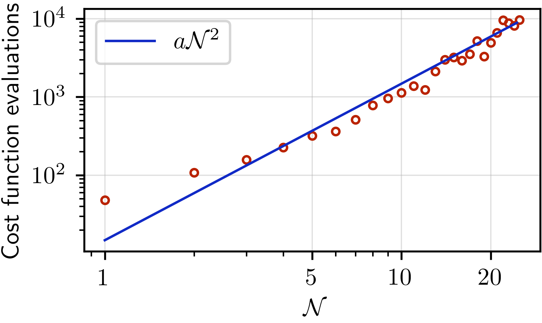
The observed exponential scaling of with implies that classical optimization over exponentially many variational parameters is required. This is highly costly and poses the primary bottleneck for reaching larger system sizes with adaptive VQE-X. In Fig. 7, we plot the number of cost function evaluations needed to complete the Nelder-Mead optimization as a function of the number of variational parameters during the early iterations of an implementation of adaptive VQE-X for the nonintegrable MFIM with . The red curve is a quadratic fit to the data, indicating that the number of cost function evaluations grows roughly as the square of the number of parameters. As scales exponentially with , it takes 200 iterations and cumulatively cost function evaluations, each one of which is made of hundreds of matrix-vector multiplications, in order to converge to an eigenstate. To further demonstrate this, we compare in Fig. 8 the adaptive VQE-X results for the integrable TFIM and nonintegrable MFIM with . Within 120 iterations, nearly 80 trials converged for the TFIM using , with a wide coverage of the energy spectrum. On the other hand, only about 10 trials converged to a few eigenstates using for the MFIM.
Indeed, the challenge of excessively many variational parameters is likely to face any variational algorithm that attempts to approximate individual finite-energy-density eigenstates of generic local Hamiltonians. Indeed, generic quantum states, of which such highly excited eigenstates are believed to be representative examples, require exponentially many gates to prepare Nielsen and Chuang 2002. Our results in Sec. IV corroborate this intuition; they show that the adaptive FSM approach yields circuits with a similar number of variational parameters on average as those produced within adaptive VQE-X. It would be interesting to see whether applying the same methodology to other cost functions capable of identifying arbitrary eigenstates, such as the “eigenstate witness” proposed in Ref. Santagati et al. 2018, could potentially yield shorter circuits or an increased convergence rate relative to the cost functions explored here. We note, however, that this cost function is difficult to implement for many-body systems on NISQ devices, as it involves an ancilla qubit, a controlled- operation, and full tomography of the ancilla. Additionally, an exponentially long evolution time is necessary to resolve the exponentially small gaps in the middle of the spectrum. In any case, finding strategies to reduce the number of variational parameters—e.g., by modifying the operator pool or foregoing the adaptive strategy in favor of a fixed family of ansätze—will be crucial for making further progress on this problem.
While our results demonstrate that approximating individual highly excited eigenstates is a challenging task, they still provide some encouraging indications that quantum algorithms could be used to study highly excited states of quantum many-body systems. For example, Fig. 1(c) demonstrates that adaptive VQE-X can be used to reproduce averages over an energy window of quantities of interest such as the entanglement entropy. This suggests that one could potentially modify the adaptive VQE-X algorithm to provide states that serve as estimators of microcanonical averages of observables and entanglement measures at finite energy density. Such a strategy should be feasible in systems obeying the strong ETH, where expectation values of observables for any eigenstate in a fixed energy window are expected to match averages over a Gibbs ensemble at a corresponding temperature, up to corrections that vanish in the thermodynamic limit Deutsch 1991; Srednicki 1994; Rigol et al. 2008; D’Alessio et al. 2016; Deutsch 2018. Whether such an estimator can be constructed using, e.g., a fixed variational ansatz with polynomially many parameters, such as the Hamiltonian variational ansatz of Ref. Wiersema et al. 2020, is an interesting question for future work. Alternatively, converged adaptive VQE-X trials can potentially serve as a basis for computing microcanonical averages. For example, given a converged variational state , one can construct a state , where is some (local) Hermitian operator. For sufficiently small , the state admixes with states nearby in energy. Taking expectation values of local operators in this state and averaging over and choices of operators may allow for a better approximation of microcanonical averages than the state alone.

Another potential avenue for future work is to use (adaptive) VQE-X to study highly excited states of disordered quantum many-body systems. When disorder is sufficiently strong, such systems are believed to enter a many-body localized (MBL) phase Abanin et al. 2019 in which emergent local conserved quantities render even highly excited states area-law entangled Serbyn et al. 2013; Bauer and Nayak 2013; Huse et al. 2014. The reduced entanglement of highly excited states in such systems may make them more amenable to representation by compact variational ansätze—indeed, this fact also enables classical simulation of such systems using tensor network approaches Khemani et al. 2016; Pollmann et al. 2016. Highly excited states with low entanglement also arise in models with quantum many-body scars Turner et al. 2018; Moudgalya et al. 2018; Schecter and Iadecola 2019. A variant of (adaptive) VQE-X (or the FSM) can be envisioned in which the cost function also contains an entanglement witness, such as the quantum Fisher information Pezzé and Smerzi 2009, such that the algorithm seeks to minimize both the entanglement and the energy variance of the variational state, potentially providing circuit representations of (rare) low-entanglement states in the spectrum.
Note Added: The data and source code used for this work have been made publicly available Zhang et al. 2021b.
Acknowledgements.
This material is based upon work supported by the National Science Foundation under Grant No. DMR-2038010 (T.I. and P.P.O.). F.Z., N.G. and Y.Y. were supported by the U.S. Department of Energy (DOE), Office of Science, Basic Energy Sciences, Division of Materials Sciences and Engineering, and performed the research at the Ames Laboratory, which is operated for the U.S. DOE by Iowa State University under Contract DE-AC02-07CH11358.References
- Preskill (2018) J. Preskill, Quantum 2, 79 (2018).
- Bharti et al. (2021) K. Bharti, A. Cervera-Lierta, T. H. Kyaw, T. Haug, S. Alperin-Lea, A. Anand, M. Degroote, H. Heimonen, J. S. Kottmann, T. Menke, W.-K. Mok, S. Sim, L.-C. Kwek, and A. Aspuru-Guzik, (2021), arXiv:2101.08448 [quant-ph] .
- Cerezo et al. (2020) M. Cerezo, A. Arrasmith, R. Babbush, S. C. Benjamin, S. Endo, K. Fujii, J. R. McClean, K. Mitarai, X. Yuan, L. Cincio, and P. J. Coles, (2020), arXiv:2012.09265 [quant-ph] .
- Peruzzo et al. (2014) A. Peruzzo, J. McClean, P. Shadbolt, M.-H. Yung, X.-Q. Zhou, P. J. Love, A. Aspuru-Guzik, and J. L. O’Brien, Nat. Comm. 5, 1 (2014).
- McClean et al. (2016) J. R. McClean, J. Romero, R. Babbush, and A. Aspuru-Guzik, New Journal of Physics 18, 023023 (2016).
- Kandala et al. (2017) A. Kandala, A. Mezzacapo, K. Temme, M. Takita, M. Brink, J. M. Chow, and J. M. Gambetta, Nature 549, 242 (2017).
- O’Malley et al. (2016) P. J. J. O’Malley, R. Babbush, I. D. Kivlichan, J. Romero, J. R. McClean, R. Barends, J. Kelly, P. Roushan, A. Tranter, N. Ding, B. Campbell, Y. Chen, Z. Chen, B. Chiaro, A. Dunsworth, A. G. Fowler, E. Jeffrey, E. Lucero, A. Megrant, J. Y. Mutus, M. Neeley, C. Neill, C. Quintana, D. Sank, A. Vainsencher, J. Wenner, T. C. White, P. V. Coveney, P. J. Love, H. Neven, A. Aspuru-Guzik, and J. M. Martinis, Phys. Rev. X 6, 031007 (2016).
- Colless et al. (2018) J. I. Colless, V. V. Ramasesh, D. Dahlen, M. S. Blok, M. E. Kimchi-Schwartz, J. R. McClean, J. Carter, W. A. de Jong, and I. Siddiqi, Phys. Rev. X 8, 011021 (2018).
- Grimsley et al. (2019) H. R. Grimsley, S. E. Economou, E. Barnes, and N. J. Mayhall, Nat. Commun. 10, 3007 (2019).
- Wecker et al. (2015) D. Wecker, M. B. Hastings, and M. Troyer, Phys. Rev. A 92, 042303 (2015).
- Ho and Hsieh (2019) W. W. Ho and T. H. Hsieh, SciPost Physics 6, 029 (2019).
- Matos et al. (2021) G. Matos, S. Johri, and Z. Papić, PRX Quantum 2, 010309 (2021).
- Klco et al. (2018) N. Klco, E. F. Dumitrescu, A. J. McCaskey, T. D. Morris, R. C. Pooser, M. Sanz, E. Solano, P. Lougovski, and M. J. Savage, Phys. Rev. A 98, 032331 (2018).
- Kokail et al. (2019) C. Kokail, C. Maier, R. van Bijnen, T. Brydges, M. K. Joshi, P. Jurcevic, C. A. Muschik, P. Silvi, R. Blatt, C. F. Roos, et al., Nature 569, 355 (2019).
- McClean et al. (2017) J. R. McClean, M. E. Kimchi-Schwartz, J. Carter, and W. A. de Jong, Phys. Rev. A 95, 042308 (2017).
- Stair et al. (2020) N. H. Stair, R. Huang, and F. A. Evangelista, J. Chem. Theory Comput. 16, 2236 (2020).
- Nakanishi et al. (2019) K. M. Nakanishi, K. Mitarai, and K. Fujii, Phys. Rev. Research 1, 033062 (2019).
- Parrish et al. (2019) R. M. Parrish, E. G. Hohenstein, P. L. McMahon, and T. J. Martínez, Phys. Rev. Lett. 122, 230401 (2019).
- Higgott et al. (2019) O. Higgott, D. Wang, and S. Brierley, Quantum 3, 156 (2019).
- Hastings (2007) M. B. Hastings, J Stat. Mech.: Theory Exp. 2007, P08024 (2007).
- White (1992) S. R. White, Phys. Rev. Lett. 69, 2863 (1992).
- Schollwöck (2011) U. Schollwöck, Ann. Phys. January 2011 Special Issue, 326, 96 (2011).
- Deutsch (1991) J. M. Deutsch, Phys. Rev. A 43, 2046 (1991).
- Srednicki (1994) M. Srednicki, Phys. Rev. E 50, 888 (1994).
- Rigol et al. (2008) M. Rigol, V. Dunjko, and M. Olshanii, Nature 452, 854 (2008).
- D’Alessio et al. (2016) L. D’Alessio, Y. Kafri, A. Polkovnikov, and M. Rigol, Adv. Phys. 65, 239 (2016).
- Deutsch (2018) J. M. Deutsch, Reports on Progress in Physics 81, 082001 (2018).
- Deutsch (2010) J. Deutsch, New Journal of Physics 12, 075021 (2010).
- Garrison and Grover (2018) J. R. Garrison and T. Grover, Phys. Rev. X 8, 021026 (2018).
- Page (1993) D. N. Page, Phys. Rev. Lett. 71, 1291 (1993).
- Luitz et al. (2015) D. J. Luitz, N. Laflorencie, and F. Alet, Phys. Rev. B 91, 081103 (2015).
- Naldesi et al. (2016) P. Naldesi, E. Ercolessi, and T. Roscilde, SciPost Phys. 1, 010 (2016).
- Nag and Garg (2017) S. Nag and A. Garg, Phys. Rev. B 96, 060203 (2017).
- Wei et al. (2019) X. Wei, C. Cheng, G. Xianlong, and R. Mondaini, Physical Review B 99, 165137 (2019).
- Zhang et al. (2021a) L. Zhang, Y. Ke, W. Liu, and C. Lee, Phys. Rev. A 103, 023323 (2021a).
- Schecter et al. (2018) M. Schecter, T. Iadecola, and S. Das Sarma, Phys. Rev. B 98, 174201 (2018).
- De Roeck et al. (2016) W. De Roeck, F. Huveneers, M. Müller, and M. Schiulaz, Phys. Rev. B 93, 014203 (2016).
- Crowley and Chandran (2020) P. J. D. Crowley and A. Chandran, Phys. Rev. Research 2, 033262 (2020).
- Brighi et al. (2020) P. Brighi, D. A. Abanin, and M. Serbyn, Phys. Rev. B 102, 060202 (2020).
- Sala et al. (2020) P. Sala, T. Rakovszky, R. Verresen, M. Knap, and F. Pollmann, Phys. Rev. X 10, 011047 (2020).
- Khemani et al. (2020) V. Khemani, M. Hermele, and R. Nandkishore, Phys. Rev. B 101, 174204 (2020).
- Turner et al. (2018) C. J. Turner, A. A. Michailidis, D. A. Abanin, M. Serbyn, and Z. Papić, Nat. Phys. 14, 745 (2018).
- Moudgalya et al. (2018) S. Moudgalya, N. Regnault, and B. A. Bernevig, Phys. Rev. B 98, 235156 (2018).
- Schecter and Iadecola (2019) M. Schecter and T. Iadecola, Phys. Rev. Lett. 123, 147201 (2019).
- MacDonald (1934) J. MacDonald, Phys. Rev. 46, 828 (1934).
- Wang and Zunger (1994) L.-W. Wang and A. Zunger, J. Comp. Phys. 100, 2394 (1994).
- Santagati et al. (2018) R. Santagati, J. Wang, A. A. Gentile, S. Paesani, N. Wiebe, J. R. McClean, S. Morley-Short, P. J. Shadbolt, D. Bonneau, J. W. Silverstone, D. P. Tew, X. Zhou, J. L. O’Brien, and M. G. Thompson, Science Advances 4, eaap9646 (2018).
- Zhang et al. (2020) D.-B. Zhang, Z.-H. Yuan, and T. Yin, (2020), arXiv:2006.15781 [quant-ph] .
- Tang et al. (2020) H. L. Tang, V. O. Shkolnikov, G. S. Barron, H. R. Grimsley, N. J. Mayhall, E. Barnes, and S. E. Economou, (2020), arXiv:1911.10205 [quant-ph] .
- Claudino et al. (2020) D. Claudino, J. Wright, A. J. McCaskey, and T. S. Humble, Front. Chem. 8, 606863 (2020).
- Ryabinkin et al. (2020) I. G. Ryabinkin, R. A. Lang, S. N. Genin, and A. F. Izmaylov, J. Chem. Theory Comput. 16, 1055 (2020).
- Gomes et al. (2021) N. Gomes, A. Mukherjee, F. Zhang, T. Iadecola, C.-Z. Wang, K.-M. Ho, P. P. Orth, and Y.-X. Yao, (2021), arXiv:2102.01544 [physics.chem-ph] .
- Yao et al. (2021) Y.-X. Yao, N. Gomes, F. Zhang, C.-Z. Wang, K.-M. Ho, T. Iadecola, and P. P. Orth, PRX Quantum 2, 030307 (2021).
- Kim and Huse (2013) H. Kim and D. A. Huse, Phys. Rev. Lett. 111, 127205 (2013).
- Kim et al. (2014) H. Kim, T. N. Ikeda, and D. A. Huse, Phys. Rev. E 90, 052105 (2014).
- Ryabinkin et al. (2018a) I. G. Ryabinkin, S. N. Genin, and A. F. Izmaylov, J. Chem. Theory Comput. 15, 249 (2018a).
- Ryabinkin et al. (2018b) I. G. Ryabinkin, S. N. Genin, and A. F. Izmaylov, J. Chem. Phys. 149, 214105 (2018b).
- Nielsen and Chuang (2002) M. A. Nielsen and I. Chuang, Quantum computation and quantum information (Cambridge University Press, New York, 2002).
- Wiersema et al. (2020) R. Wiersema, C. Zhou, Y. de Sereville, J. F. Carrasquilla, Y. B. Kim, and H. Yuen, PRX Quantum 1, 020319 (2020).
- Abanin et al. (2019) D. A. Abanin, E. Altman, I. Bloch, and M. Serbyn, Rev. Mod. Phys. 91 (2019).
- Serbyn et al. (2013) M. Serbyn, Z. Papić, and D. A. Abanin, Phys. Rev. Lett. 111, 127201 (2013).
- Bauer and Nayak (2013) B. Bauer and C. Nayak, J. Stat. Mech.: Theory Exp. 2013 (09), P09005.
- Huse et al. (2014) D. A. Huse, R. Nandkishore, and V. Oganesyan, Phys. Rev. B 90, 174202 (2014).
- Khemani et al. (2016) V. Khemani, F. Pollmann, and S. L. Sondhi, Phys. Rev. Lett. 116, 247204 (2016).
- Pollmann et al. (2016) F. Pollmann, V. Khemani, J. I. Cirac, and S. L. Sondhi, Phys. Rev. B 94, 041116 (2016).
- Pezzé and Smerzi (2009) L. Pezzé and A. Smerzi, Phys. Rev. Lett. 102, 100401 (2009).
- Zhang et al. (2021b) F. Zhang, N. Gomes, Y. Yao, P. P. Orth, and T. Iadecola, Adaptive variational quantum eigensolvers for highly excited states (2021b).