Non-Gaussian Quantum States and Where to Find Them
Abstract
Gaussian states have played on important role in the physics of continuous-variable quantum systems. They are appealing for the experimental ease with which they can be produced, and for their compact and elegant mathematical description. Nevertheless, many proposed quantum technologies require us to go beyond the realm of Gaussian states and introduce non-Gaussian elements. In this Tutorial, we provide a roadmap for the physics of non-Gaussian quantum states. We introduce the phase-space representations as a framework to describe the different properties of quantum states in continuous-variable systems. We then use this framework in various ways to explore the structure of the state space. We explain how non-Gaussian states can be characterised not only through the negative values of their Wigner function, but also via other properties such as quantum non-Gaussianity and the related stellar rank. For multimode systems, we are naturally confronted with the question of how non-Gaussian properties behave with respect to quantum correlations. To answer this question, we first show how non-Gaussian states can be created by performing measurements on a subset of modes in a Gaussian state. Then, we highlight that these measured modes must be correlated via specific quantum correlations to the remainder of the system to create quantum non-Gaussian or Wigner-negative states. On the other hand, non-Gaussian operations are also shown to enhance or even create quantum correlations. Finally, we will demonstrate that Wigner negativity is a requirement to violate Bell inequalities and to achieve a quantum computational advantage. At the end of the Tutorial, we also provide an overview of several experimental realisations of non-Gaussian quantum states in quantum optics and beyond.
I Introduction
Gaussian states have a long history in quantum physics, which dates back to Schrödinger’s introduction of the coherent state as a means to study the harmonic oscillator Schrödinger 1926. In later times, Gaussian states rose to prominence due to their importance in the description of Bose gases Araki and Woods 1963; Robinson 1965; Verbeure 2011 and in the theory of optical coherence Glauber 1963; Sudarshan 1963. With the advent of quantum information theory, the elegant mathematical structure of Gaussian states made them important objects in the study of continuous-variable (CV) quantum information theory Braunstein and van Loock 2005; Weedbrook et al. 2012; Adesso et al. 2014. In this Tutorial, we focus on bosonic systems which means that the continuous variables of interest are field quadratures. Gaussian quantum states are then defined as the states for which measurement statistics of these field quadratures is Gaussian.
Gaussian states can be fully described by their mean field and covariance matrix, and, due to Williamson’s decomposition Williamson 1936, the latter can be studied using a range of tools from symplectic vector spaces. As such, one can directly relate quadrature squeezing to Gaussian entanglement via the Bloch-Messiah decomposition Braunstein 2005. In the full state space of CV systems, Gaussian states are furthermore known to play a specific role: of all possible states with the same covariance matrix, the Gaussian state will always have the weakest entanglement Wolf et al. 2006 and the highest entropy Holevo et al. 1999. From a theoretical point of view, Gaussian quantum states provide, thus, an elegant and highly relevant framework for quantum information theory. On an experimental level, CV quantum information has long been motivated by advances in quantum optics, due to the capability of on-demand generation of ever larger entangled states using either spatial modes Yukawa et al. 2008; Su et al. 2012; Barral et al. 2020 or time-frequency modes Roslund et al. 2014; Chen et al. 2014; Cai et al. 2017; Asavanant et al. 2019; Larsen et al. 2019; Yang et al. 2021. Furthermore, Gaussian states also play a key role in the recent demonstration of a quantum advantage with Gaussian Boson Sampling Zhong et al. 2020. These developments have made the CV quantum optics an important platform for quantum computation Bourassa et al. 2021.
Regardless of all the experimental and theoretical successes of Gaussian states, they have a major shortcoming in the context of quantum technologies: all Gaussian measurements of such states can be efficiently simulated Bartlett et al. 2002. In pioneering work on CV quantum computation, it is already argued that a non-Gaussian operation is necessary to implement a universal quantum computer in CV Lloyd and Braunstein 1999. Later works that laid the groundwork for CV measurement-based quantum computing have left the question of this non-Gaussian operation somewhat in the open Menicucci et al. 2006; Gu et al. 2009; Menicucci 2014. Common schemes, based on the cubic phase gate, turn out to be particularly hard to implement in realistic setups Arzani et al. 2017. Furthermore, these protocols require highly non-Gaussian states, such as Gottesman-Kitaev-Preskill (GKP) states Gottesman et al. 2001, to encode information. Even though such states could also serve as a non-Gaussian resource for implementing non-Gaussian gates Baragiola et al. 2019, these states remain notoriously challenging to produce. In spite of the practical problems involved with non-Gaussian states, one is obliged to venture into non-Gaussian territory to reach a quantum computational advantage in the CV regime Mari and Eisert 2012. This emphasises the importance of a general understanding of non-Gaussian states and their properties. In this Tutorial, we attempt to provide a roadmap to navigate within this quickly developing field.
In Section II, we take an unusual start to introduce CV systems. We first present some elements many-boson physics, by treating Fock space. This mathematical environment is probably familiar to most readers to describe photons. We then explain how such a Fock space can also be described in phase space, which is the more natural framework from CV quantum optics. We will introduce phase-space representations of states and observables in CV systems such as the Wigner function, and to familiarise the reader with the language of multimode systems. By first reviewing the basics of Fock space, we can make interesting connections between what is known as the discrete-variable (DV) approach and the CV approach to quantum optics. We will see that there is often a shady region between these two frameworks, where techniques that are typically associated with one framework can be applied in the other.We will finally argue that the main distinction lies in whether one measures photons (DV) or field quadratures (CV).
In Section III, we provide the reader with an introduction to some of the different structures that can be identified in the space of CV quantum states. When pure states are considered, all non-Gaussian states are known to have a non-positive Wigner function Hudson 1974; Soto and Claverie 1983, but this no longer holds when mixed states enter the game Mandilara et al. 2009. In the entirety of the state space, non-Gaussian states occupy such a vast territory that it is impossible to describe all of them within one single formalism. Nevertheless, there has recently been considerable progress in the classification of non-Gaussian states Lachman et al. 2019; Chabaud et al. 2020. We will introduce some key ideas behind quantum non-Gaussianity, the stellar rank, and Wigner negativity as tools to characterise non-Gaussian states.
Section IV introduces two main families of techniques to create non-Gaussian states starting from Gaussian inputs. The first approach concentrates on deterministic methods, which rely on the implementation of non-Gaussian unitary transformations. We will show how such transformations can be built by using a specific non-Gaussian gate. We then introduce the second class of techniques which are probabilisitic and rely on performing non-Gaussian measurements on a Gaussian state and conditioning on a certain measurement result. We introduce our recently developed approach to describe these systems Walschaers et al. 2020 and present mode-selective photon subtraction as a case study.
Then all the pieces are set to discuss the interplay between non-Gaussian effects and quantum correlations in Section V. First, we will consider the resources that are required to conditionally prepare certain non-Gaussian states. The conditional scheme relies on performing a non-Gaussian measurement on one part of a bipartite Gaussian state, and will show that the nature of the quantum correlations in this bipartite state is essential. We will show that we can only generate quantum non-Gaussian states if the initial bipartite state is entangled. Furthermore, to conditionally generate Wigner negativity we even require quantum steering. In the second part of Section V, we show how non-Gaussian operations can in return enhance or create quantum correlations. Finally, we will show that Wigner negativity (in either the state or the measurement) is necessary to violate Bell inequalities in CV systems.
In a similar fashion, we will spend most of Section VI to explain the result of Ref. Mari and Eisert 2012, which shows that Wigner negativity is also necessary to reach a quantum advantage. To show this, we explicitly construct a protocol to efficiently simulate the measurement outcomes of a setup with states, operations, and detectors that are described by positive Wigner functions. In the remainder of the section, we provide comments on the quantum computational advantage reached with Gaussian Boson Sampling.
Finally, in Section VII, we provide a quick overview of non-Gaussian states in CV experiments. Due to the author’s background, the first half of this overview will focus on quantum optics.In the second part, we also discuss some key developments in other branches of experimental quantum physics. Readers should be warned that this is by no means an extensive review of all the relevant experimental progress. A more general conclusion and outlook on what the future may have in store is presented in Section VIII.
II Continuous-Variable Quantum States
Before we can start our endeavour to classify non-Gaussian states of CV systems and study their properties, we must develop some basic formalism for dealing with multimode bosonic systems. At the root of bosonic systems lies the canonical commutation relation, , which can be traced back to the early foundations of quantum mechanics. The study of the algebra of such non-commuting observables has given birth to rich branches of mathematics and mathematical physics that ponder on the subtleties of these observables and their associated states. In this Tutorial, we will keep a safe distance from the representation theory of the associated -algebras that describes bosonic field theories in their most general sense. We do refer interested readers to a rich but technical literature Verbeure 2011; Petz 1990; Bratteli and Robinson 1987; Bratteli and Robinson 1997.
In this Tutorial, we will exclusively work within the Fock representation, which implies that we consider systems with a finite expectation value for the number of particles. In quantum optics, this assumption translates to the logical requirement that energies remain finite. There are many approaches to mathematically construct such systems (luckily for us they are all equivalent Stone 1930; von Neumann 1931; Stone 1932; von Neumann 1932). Here, we briefly present two such approaches that nicely capture one of the key dualities on quantum physics. First we will take the particle approach by introducing the Fock space that describes identical bosonic particles in Subsection II.1. Subsequently, in Subsection II.2, we take the approach that starts out from a wave-picture, by concentrating on the phase-space representation of the electromagnetic field. Here we will also introduce the phase-space representations of CV quantum states that will prove to be crucial tools in the remainder of this Tutorial. We will show how these approaches are quite naturally two sides of the same coin. In Subsection II.3, we briefly discuss the concept of modes and the role they play in CV quantum systems. This subsection is both intended to provide some clarification about common jargon and to eliminate common misconceptions. We finish this section by presenting a brief case study of Gaussian states in Subsection II.4, reviewing some key results. After all, it is difficult to appreciate the subtleties of non-Gaussian states without having a flavour from their Gaussian counterparts.
II.1 Fock Space
In typical quantum mechanics text books, the story of identical particles usually starts by considering a set of particles, which are each described by a quantum state vector in a single-particle Hilbert space , thus for the th particle we ascribe a state vector . The joint state of these particles is then given by the tensor product of the state vectors . However, if the particles are identical in all their internal degrees of freedom, we should be free to permute them without changing the observed physics. Formally, such permutation is implemented by a unitary operator , for the permutation , which acts as
| (1) |
Invariance of physical observables under such permutations can be achieved by either imposing the -particle states vector to be fully symmetric (bosons) or fully antisymmetric (fermions) under these permutations of particles. In this Tutorial, we focus exclusively on bosons, and thus the condition that must be imposed to obtain a bosonic -particle state is
| (2) |
Because these are the only states that are permitted to described the bosonic system, we commonly use the Hilbert space which is a subspace of that contains only those states that fulfil (2). It is usually convenient to generate these spaces with a set of elementary tensors, known as Fock states, which we define as
| (3) |
such that
| (4) |
where we refer to Appendix A.2 for some further details on the span. This fully describes a system of bosonic particles in what is often referred to as first quantisation. It is interesting to note that these identical particles appear to be entangled with respect to the tensor product structure of . There is still debate on whether this is a mathematical artefact of our description or rather a genuine physical feature of identical particles Morris et al. 2020. Nevertheless, it is undeniable that this structure leads to physical interference phenomena that do not exist for distinguishable particles Tichy 2014.
The name “first quantisation” suggests the existence of a second quantisation, which turns out to be more appropriate for this Tutorial. Second quantisation finds its origins in models where particle numbers are not fixed or conserved. This formalism is largely based on creation and annihilation operators, denoted and , respectively, that add or remove particles. To accommodate these operators in our mathematical framework, we must equip our Hilbert space to describe a varying number of particles. Therefore, we introduce the Fock space
| (5) |
where the single-particle Hilbert space is given by . Furthermore, we retrieve a peculiar component which describes the fraction of the system that contains no particles at all. On its own, is thus populated by a single state that we refer to as the vacuum. This implies that technically the zero-particle Hilbert space is just described by a complex number that corresponds to the overlap of the state with the vacuum. A general pure state in Fock space can then be described using the structure (5) as
| (6) |
where are non-normalised vectors (and therefore we omit the ) in the -particle Hilbert space. Because is a state, we must impose the normalisation condition
We can now define a creation operator for every 11 1 Note that the notation is not a coincidence, we can indeed construct a formal linear map from the single-particle Hilbert space into the operator algebra of linear operators on the Fock space. This mapping takes single-particle state vectors and maps them to a creation operators. The mapping is linear in the sense that , for all , which acts as
| (7) |
In the same spirit, it is possible to provide an explicit construction of the annihilation operators , but here we will content ourselves by just introducing the annihilation operator as the hermitian conjugate of the creation operator. Just as the creation operator that literally adds a particle to the system, the annihilation operator literally removes one. One additional property of the annihilation operators is that they destroy the vacuum state:
| (8) |
We can now use creation and annihilation operators to build an arbitrary Fock state by creating particles on the vacuum state
| (9) |
and by considering superpositions of such Fock states, we can ultimately generate the entire Fock space. By considering any basis of the single-particle Hilbert space and constructing all possible Fock states of all possible lengths that can be formed by generating particles in these basis vectors we construct a basis of the Fock space . We refer to this basis as the Fock basis.
The beauty of second quantisation lies in the natural appearance of states which have no fixed particle number. The most important example is the coherent state
| (10) |
where is a non-normalised vector in the single particle Hilbert space. One can, indeed, simply generalise (7) to non-normalised vectors in which we use explicitly in (10). Second, we note that an unusual factor was included to make the definition consistent with (62).
In quantum optics, these ciherent states are crucial objects as they describe perfectly coherent light Glauber 1963. It is important to remark that a coherent state is always generated by a single vector in the single-particle Hilbert space. Coherent states often provides a good approximation for the state that is produced by a single-mode laser far above threshold Mandel and Wolf 1995. More generally, the study of laser light is a whole field in its own right and often the light deviates from the fully coherent approximation.
The creation and annihilation operators are not only important objects because they populate the Fock space; they are also of key importance for describing observables in a many-boson system. These operators are the generators of the algebra of observables that represents the canonical commutation relations on Fock space. This implies that any observable can ultimately be approximated by a polynomial of creation and annihilation operators. At the heart of this mathematical formalism lies the canonical commutation relation (CCR):
| (11) |
which describes the algebra of observables. Note that this relation holds for any vectors and in the single-particle Hilbert space . These vectors should not form a basis, nor should they be orthogonal. When , we find that . On the other hand, when the single-particle states and are fully orthogonal, we find that . In these cases we recover the typical creation and annihilation operators for harmonic oscillators. However, by introducing the creations and annihilation operators through (7), we can also deal with more general cases. Furthermore, all definitions and the form of the CCR are still valid when and are unnormalised vectors in . A more detailed discussion can be found in Walschaers 2020.
When we leave the realm of pure states, the description of quantum states becomes tedious. Commonly, one uses a density operator with to formally describe a state. However, we can generally think of these density operators as infinite-dimensional matrices with an infinite number of components in the Fock basis. In other words, this is not necessarily a convenient description. In an operational sense, any state is considered to be characterised when we know all the moments of all the possible observables. Because the creation and annihilation operators generate the algebra, one knows all the moments of all the observables if one knows all the correlation functions , for all possible lengths and . Even though this might seem like an equally challenging endeavour, much of quantum statistical mechanics boils down to finding expressions of the correlation functions for relevant classes of states.
II.2 Phase Space
In the previous subsection, we started our analysis by extending a system of one quantum particle to a system of many quantum particles. Here we follow a different route, where we start by considering the classical electric field. With some effort, we can apply such an analysis to any bosonic field, but in this Tutorial we focus on quantum optics as our main field of application. For a more extensive introduction from a quantum optics perspective we recommend Ref. Mandel and Wolf 1995; Schleich 2001a; Fabre and Treps 2020, whereas a general introduction to quantum physics in phase space can be found in Ref. de Almeida 1998.
A travelling electromagnetic wave is described by a solution of Maxwell’s equations. As is commonly the case in optics, we focus on the complex representation of the electric field which is generally given by . It is related to the real-valued electric field that is encountered in standard electrodynamics textbooks by . To express the electric field, it is useful to introduce an orthonormal mode basis . These modes are solutions to Maxwell’s equations
| (12) | ||||
| (13) |
The orthogonalisation property is implemented by the following condition
| (14) |
where is some large volume that contains the entire physical system. This assumption serves the practical purpose of allowing us to consider a discrete mode basis and on top it makes physical sense. Note that we do not integrate over , which implies that at every instant of time we consider a mode basis that is normalised with respect to the spatial degrees of freedom. It is practical to assume that all relevant physics can be described by a (possibly large) finite number of modes . These modes now form a basis in which we can expand any solution to Maxwell’s equations and thus we may write
| (15) |
where are a set of complex numbers which can be written in terms of the real and imaginary parts
| (16) |
These real and imaginary parts of the field are known as the amplitude and phase quadrature, respectively. We can interpret these quantities as the coordinate in optical phase space that describes the light field.
The space of solutions of Maxwell’s equations forms a Hilbert space which we will call the mode space and the mode basis chosen to describe this space is far from unique. As with all Hilbert spaces, we can define unitary transformations and use them to change from one basis to another. As such, let us introduce the unitary operator to change between bases
| (17) | ||||
| (18) |
where we can in principle obtain as an infinite-dimensional matrix with
| (19) |
which remarkably does not depend on time due to the normalisation properties of the mode bases. We can analogously expand the electric field in the new mode basis
| (20) |
where . This observation is of great importance when we quantise the electric field. The change of mode basis also imposes a change of coordinates in the optical phase space. Like in (16) the new components can also be divided in real and imaginary parts, which leads to a new coordinate . Because the coordinate vectors in optical phase space are real -dimensional vectors, we obtain
| (21) |
where is an orthonormal transformation. However, the orthogonal transformation on the phase space must correspond to the unitary transformation on the modes, which imposes the constraint
| (22) | ||||
| (23) | ||||
| (24) | ||||
| (25) |
This imposes a symplectic structure to the transformation such that the optical phase space, just like the phase space of analytical mechanics, can be treated as a symplectic space. The conserved symplectic structure associated with this space is given by
| (26) |
such that . Note that can be interpreted as a matrix representation of the imaginary , in the sense that it has the properties and 22
2
In literature, one will encounter various different choices for the symplectic structure which correspond to different forms of ordering the amplitude and phase quadratures. In general, any matrix that satisfies the conditions and defines a symplectic structure. A popular alternative to the ordering that we follow in this Tutorial is the ordering . The choice in this Tutorial is motivated by the study of entanglement, where it is more convenient to group the quadratures that correspond to the same modes together..
In quantum optics, the electric field of light is treated as a quantum observable . In this quantisation, the modes, i.e., the normalised solutions to Maxwell’s equations, remain classical objects and all the quantum features are absorbed in the coefficients. We can thus write
| (27) |
where is a constant that carries the dimensions of the field, which can be interpreted as the electric field of a single photon. Glossing over many subtleties of the quantisation of the electromagnetic field, we recall the reader that any system that is described on phase space can be quantised through canonical quantisation. The quadrature operators and therefore follow the canonical commutation relations , such that they satisfy the Heisenberg relation . As they are introduced above, the quadrature operators are specifically related to the specific mode basis. Indeed, and are the quadrature operators that describe the field in mode . Thus, when we change the basis of modes, we should change the quadrature operators accordingly in line with (21). To overcome these difficulties, it is often convenient to introduce a basis-independent expression for the quadrature operators, which can be done by mapping any point in the optical phase space to an observable , given by
| (28) |
These quadrature operators follow a generalised version of the canonical commutation relation (CCR), given by
| (29) |
We highlight the particular case where , such that we recover the typical form of the CCR for . This highlights that maps an amplitude quadrature to its associated phase quadrature. From a mathematical point of view, everything is perfectly well-defined for arbitrary and no normalisation conditions have to be imposed. From (28) we can see that the norm of can be factored out, such that it serves as general rescaling factor of the quadrature operator. In a physical context, when a quadrature is measured, it is common to renormalise measurements to units of vacuum noise, which practically means that we set . Unless explicitly stated otherwise, we assume that throughout this Tutorial. We can use these general quadrature operators to express electric field operator as
| (30) |
and we can use the basis transformation (21) to equivalently express the electric field operator in a different mode basis as
| (31) |
This procedure shows us that optical elements, that change the mode basis, change the associated quadrature operators accordingly.
Equation (30) shows us explicitly that quadrature operators and correspond to the same mode, regardless of the mode basis. This reflects the fact that generates one axis in the optical phase space and generates the second axis that corresponds to the same mode. As such, any arbitrary mode comes with an associated two-dimensional phase space that mathematically can be denoted as . Because this phase space is uniquely associated with a specific mode, we introduce the notation
| (32) |
and we refer to this as “mode ”. This allows us to concentrate on the multimode quantum states within this Tutorial, while the specifications of the modes can be left ambiguous. The modes can be seen as the physical implementations of the quantum system and are of major importance in the experimental setting as multimode quantum optics experiments rely on the manipulation of these modes.
Multimode quantum states define expectation values of the field, and when we consider CV quantum optics, we primarily focus on the expectation values of the quadrature operators . These operators are unbounded and have a continuous spectrum. The measurement of a field quadrature thus leads to a continuum of possible outcomes and the continuous variable approach to quantum optics implies that this characterises quantum properties of light through the measurement of such quadrature operators.
Formally, we can again describe a quantum state on such a system by a density operator but this description is rather inconvenient. It turns out that the quadrature operators generate the algebra of observables for the quantum system that is comprised within our multimode light. In other words, any observable can be approximated by a polynomial of quadrature operators. This generally implies that we can fully characterise the quantum state by correlation functions of the type . When we know these correlation functions for all lengths and normalised vectors in phase space, we have fully characterised the state.
To go beyond the information that is contained in correlation functions, it is often convenient to consider probability distributions as a whole. For a single quadrature we can introduce the characteristic function for any as
| (33) |
which is clearly related to the moments . The characteristic function is the Fourier transform of the probability distribution of the outcomes of observable . We can thus obtain the probability distribution as
| (34) |
This approach can be readily generalised to the joint probability distribution for a set of commuting quadrature operators. We thus consider with for all , and we define for all (note that is not normalised). We can then use the properties of the quadrature operators to construct and define the function
| (35) |
This function generates all the correlations between observables and it can be used to obtain the multivariate probability distribution
| (36) |
where . The function describes the probability density to jointly obtain as measurement outcomes for the measurements of , respectively. This approach relies on the fact that commuting observables can be jointly measured and what we presented to derive (34) and (36) is ultimately just classical probability theory. However, not all quadrature operators commute such that joint measurements are not always possible. This implies that a quantum state cannot be straightforwardly defined by a probability distribution of the optical phase space.
Intriguingly, we can carry out the same procedure for a full multimode system over a set of modes. To this goal, let us define the quantum characteristic function
| (37) |
This function, defined on the full optical phase space, can be used to generate all correlation functions between all quadrature operators. As such, it does characterise the full quantum state, but it is common practice to rather study its inverse Fourier transform which is known as the Wigner function Wigner 1932; Hillery et al. 1984; Schleich 2001b
| (38) |
This function has many appealing properties even though it is not a probability distribution but rather a quasiprobability distribution. First of all, the Wigner function is normalised, i.e., . Furthermore, its marginals consistently describe all the joint probability distributions for sets of commuting quadratures in the system. Formally, this implies that of (36) can be obtained by integrating over all the phase space axes that are not contained within . To do so, let us introduce the -dimensional vector that is associated with the measured quadratures, and the dimensional vectors which describe all other axes in phase space. An arbitrary point in phase space can thus be written as . Then we find that
| (39) |
Finally, the Wigner function also produces the correct expectation values
| (40) |
Note that considering the real part of is essentially equivalent to considering symmetric ordering of the operators. Regardless of these nice properties the Wigner function is by itself not a well-defined probability distribution. Due to complementarity, the function can reach negative values for some states. This Wigner negativity is consistent with the impossibility to jointly describe the measurement statistics of all quadratures while also complying with the laws of quantum physics (notably the Heisenberg relation). The profound relation between negativity of the Wigner functions and joint measurability is perhaps most strikingly illustrated by its connection to contextuality Spekkens 2008. . The formalism of Wigner functions can be used to construct phase-space representations of arbitrary observables by introducing
| (41) |
such that the Wigner representation is given by
| (42) |
These Wigner representations have the appealing property that
| (43) |
When is an observable and thus has , its Wigner function will be real such that . However, it may sometimes be useful to extend the formalism to more general operators. As such the entire theory of continuous-variable quantum systems can be developed using Wigner functions.
Several aspects of the phase-space representations in this section are reminiscent of earlier results in Section II.1 which was fully developed in a language of particles (also known as a discrete-variable approach). Indeed, the algebra of operators that is generated by the creation and annihilation operators is actually the same as the algebra generated by the quadrature operators. To formalise this, we must first stress that the optical phase space is isomorphic to an -dimensional complex Hilbert space which can equally be interpreted as the single-particle Hilbert space of a photon. Formally, this equivalence is constructed through the bijection (see also Appendix A.1)
| (44) |
where is an arbitrary basis of . We can introduce the operators
| (45) |
By using (44), we can naturally associate these operators to creation and annihilation operators on the single particle Hilbert space. We retrieve the canonical commutation relation
| (46) |
which can be connected to the inner product on the Hilbert space via (44).
The definition of creation and annihilation operators allows us to make sense of the vacuum state in our phase space picture. The vacuum state is completely characterised by the property
| (47) |
This simple fact can be used to evaluate the quantum characteristic function
| (48) | ||||
| (49) | ||||
| (50) | ||||
| (51) |
To obtain equation (50) we need a considerable amount of combinatorics to evaluate . In general, it can be shown that . Thus it suffices to cast in normal ordering and extract the term proportional to identity. Even though straightforward, this calculation is quite cumbersome and thus we do not present the details.
From (51) the Wigner function can be obtained via an inverse Fourier transformation that leads to
| (52) |
This Wigner function describes a Gaussian distribution on the phase space with unit variance along every axis. We can thus use (40) to see that the vacuum state saturates Heisenberg’s inequality, i.e., .
The quadrature operators thus generate the same algebra of observables as the creation and annihilation operators. However, both sets of observables tend to cause mathematical problems because they are unbounded operators von Neumann 1955; Weyl 1927; Conway 1985; Bratteli and Robinson 1997. The unboundedness means that, when is contained in the Fock space, there is no guarantee that will also be contain in the Fock space. One way of solving this problem explicitly is by only considering states for which , such that is a well-defined state. Physically this assumption makes sense, as it ultimately implies that we only consider states with finite energies. However, the unboundedness of quadrature operators also disqualifies them as well-defined generators of the -algebra of observables (since elements of such algebras must be bounded). -algebras are essential tools as they allow to reconstruct the whole framework of Hilbert spaces based on representation theory of abstract algebras (which is essentially the idea of canonical quantisation). A highly formal and detailed treatment that considers all these subtleties for bosonic systems is found in Bratteli and Robinson 1987. The key idea is to rather consider a set of bounded operators that describes the same algebra of observables von Neumann 1955; Weyl 1927 and are known as the displacement operators:
| (53) |
where need not be normalised. Again, we can use the isomorphism (44) to identify the displacement operator on the quantised phase space to a displacement operator on Fock space. These operators can be seen as generators of the quadrature operators and they act in a very natural way on them:
| (54) |
which means that the value is added to the measurement outcomes of . The displacement operator can be combined according to the rule
| (55) |
This rule is yet another representation of the canonical commutation relation and it generates the same algebra of observables. This implies that any observable can be written as a linear combination of displacement operators. We use the Hilbert-Schmidt inner-product to make this explicit
| (56) |
and we can readily identify that
| (57) |
It can then directly be seen that
| (58) | ||||
| (59) |
And we immediately obtain (43) via Plancherel’s theorem Plancherel 1910; Conway 1985.
The displacement operators also implement a unitary operation on a quantum state. This unitary operation has a remarkably simple effect when it is expressed on the level of the Wigner function. Via the property (55), we can calculate that
| (60) |
Performing the inverse Fourier transform of these quantum characteristic functions leads to
| (61) |
The displacement operator thus literally implements a displacement of the Wigner function by a vector in phase space.
Displacement operators are also well-known as the generators of the coherent states that were introduced in (10). We can combine the bijection between phase space and Hilbert space (44), the expression of creation and annihilation operators in terms of quadratures (45), and the definition of the displacement operator (53) to derive that
| (62) |
By combining (52) and (61), we immediately see that the Wigner function for such a coherent state is given by
| (63) |
We emphasise that there is a slight difference between the coherent states as defined here, and coherent states as sometimes introduced in literature. The difference is a factor two, which appears because we normalised the shot noise to rather than to . As such, our coherent states have an energy in mode which is given by
| (64) |
The coherent states lead us to two other representations of quantum states and observables: the Q-function and P-function. The definition of the P-function is related to the idea that coherent states form an overcomplete basis of Fock space. This implies, notably, that for a -dimensional single particle Hilbert space
| (65) |
with the identity operator. We can then show that any observable can be written as Glauber 1963; Sudarshan 1963
| (66) |
where we refer to as the P-function of the observable . Similarly, we can represent a density of operator by its P-function . The reader should be warned that P-functions often have rather unpleasant mathematical properties. In particular, they often are not actual functions and can be highly singular.
The P-function naturally comes with a dual representation that is known as the Q-function. As often in quantum physics, what actually counts is the expectation value of an observable in a specific state. We can use the P-function to write
| (67) | ||||
| (68) |
This naturally introduces the Q-function, given by
| (69) |
and in particular for the quantum state we find that
| (70) |
The latter is of particular interest because it represents the quantum state as an actual probability distribution. This leads us to the general identity that
| (71) |
Thus finishing our introduction to the various descriptions of the quantum states and observables of bosonic many-particle systems.
The Q-function has a clear physical interpretation. It is directly proportional to the fidelity of the state with respect to a target coherent state . Furthermore, it is always positive, which implies that it is a well-defined probability distribution. Because we can write , we can use (43) and (52) to express the Q-function in terms of the Wigner function as
| (72) |
To satisfy both (43) and (71), we find that
| (73) | ||||
| (74) |
In turn, this implies that
| (75) |
These results thus show that all these phase-space representations are ultimately related to one another through convolution or deconvolution with a Gaussian (recall that the Wigner function of the vacuum (52) is a Gaussian distribution on phase space). One can now follow Ref. Cahill and Glauber 1969 to define a continuous family of phase-space representations for
| (76) |
where we convolute the P-function with an ever increasing Gaussian, smoothening its features. We can then see that
| (77) |
We find, notably, that , , and . This shows that the phase-space representation becomes more regular when decreasing . Other generalised probability distributions have been considered in literature Dirac 1945; Sperling and Vogel 2020, often to circumvent the unappealing properties of the P-function. In this Tutorial, we mainly use the Wigner function and (to a lesser extent) the Q-function, as they are suitable tools to classify non-Gaussian quantum states. The P-function is often used in literature to characterise the non-classicality of a state, where the intuition is that classical light is a mixture of coherent states (and thus its P-function is a probability distribution) Glauber 1963; Sudarshan 1963.
Before we close this introductory section on the phase space description of CV quantum systems, we introduce one final tool that often comes in handy. The Wigner function can itself be obtained as the expectation value of an operator Royer 1977. Formally, we write
| (78) |
Using linearity and (38), we obtain the special case
| (79) |
By using techniques based on (54) and (55), we can show that
| (80) |
This means that is the parity operator. Its eigenstates are the Fock states, since
| (81) |
Thus we can formally identify
| (82) |
where is the number operator. We define this operator by introducing a mode basis of the optical phase space, such that . This definition can be combined with the properties of the displacement operator to obtain that
| (83) |
Note that what we just obtained is the operator equivalent of a -function, which becomes even more explicit when we explicitly write down its Wigner representation
| (84) |
This result may seem somewhat artificial, but it turns out to be extremely useful. The observable can be measured experimentally by counting photons, which means that the combination of photon counting and displacements directly allows us to reconstruct the Wigner function of the quantum state Banaszek and Wódkiewicz 1996. Up to recently, the lack of good photon-number-resolving detectors in the optical frequency range has long made this method unfeasible for most states. Even though there was an early demonstration of the method for coherent states Banaszek et al. 1999, it is only due to recent developments in detector technologies that the method the method can be applied to more general states Laiho et al. 2010; Nehra et al. 2019. The idea was also other settings Lutterbach and Davidovich 1997, and was used in pioneering CV experiments with trapped ions, such as Leibfried et al. 1996, and in cavity-QED Nogues et al. 2000; Bertet et al. 2002.
II.3 Discrete and continuous variables
In Subsection II.1, we have introduced a many-boson system, regardless of the physical realisation of these bosons. Such a many-boson system and its Fock space are built upon the structure that is determined by the single-particle Hilbert space . The Fock space that is constructed accordingly has a rich structure that is further explored in the Tutorial Walschaers 2020. In optics, the bosons that we consider are photons, and quantum optics can thus be seen as the theory of a many-boson system in the context of II.1. This approach to quantum optics is referred to as the DV approach.
In Subsection II.2, we contrast this with the CV approach to quantum optics. This approach relies on the measurement of the field quadratures, and can thus been seen as a bosonic quantum field theory. Therefore we started this approach by introducing the classical electric field and its modes, which we subsequently quantised through canonical quantisation. We introduced the notion of optical phase space as a general way of describing CV quantum systems. The phase space is directly related to the modes of the field and manipulations of the modes also cause changes in the optical phase space. Nevertheless, any system with a phase space can be described by these techniques.
Both of these approaches are ultimately equivalent. Bosonic creation and annihilation operators describe the same algebra of observables as bosonic quadrature operators, which means that on the level of mathematical structure, both approaches can be interchanged and even mixed. This is strikingly clear when the Wigner function, i.e, the phase-space representation of quantum states and observables that is most naturally associated with field quadratures, turns out to be directly measurable by counting photons. Notably, this implies that when it comes to mathematical structures, bosonic particles such as atoms can also be described on phase space.
The real difference between CV and DV approaches is of an experimental nature. What is important is not the observables that are technically present in the quantum system, but the observables that are practically measured in the lab. For the CV approach we typically use homodyne detection to measure quadratures Braunstein and van
Loock 2005; Lvovsky et al. 2020, whereas in DV approaches we count photons Flamini et al. 2018.
A common source of misunderstanding between the DV and CV community stems from the role they attribute to the single-particle Hilbert space and optical phase space, respectively. As we argued, both spaces are (at least for a finite-dimensional number of modes) isomorphic, see Appendix A.1 for some additional mathematical intuition. However, the Hilbert space of a photon, which is inherently a quantum particle, is often interpreted as a quantum object. At the same time, the optical phase space represents the field quadratures of optical modes and is thus rather considered to be a classical object. The origin of this confusion lies in the fact that the optical modes, i.e., normalised solutions of Maxwell’s equations, also form a Hilbert space that has its origins entirely in classical physics.
The optical modes are the vessels that contain photons much in the same way as a set of electrons contains spins. The crucial difference is that optical modes are not uniquely defined, we can manipulate them, transform them from one mode basis to another with an interferometer and thus consider new superpositions of modes. In typical experimental settings, one would not consider a superposition of two electrons a new well-defined electron.
Because creation and displacement operators always act in one specific mode (i.e., they are generated by a single vector on the single-photon Hilbert space), single-photon states and coherent states are always single-mode states. We may expand this single mode in a different mode basis, which can even be done physically by sending the state through a beamsplitter, to create some form of entanglement in the quantum states. However, this entanglement is just a manifestation of the fact that we are not considering the optimal mode basis. In the CV approach, this has led to the notion of “intrinsic” properties Fabre and Treps 2020, which are those properties of quantum states that are independent of the chosen mode basis. The purity and entropy of a state are notable examples, but one can also introduce a notion of “intrinsic entanglement” to refer to a state that is entangled in any possible mode basis. In the next subsection, we introduce Gaussian states which will later be shown to never be intrinsically entangled.
II.4 Gaussian States
Now that we have introduced phase-space representations for states and observables of CV quantum systems, we still need one building block before we can tackle multimode non-Gaussian states: a good understanding of Gaussian states. It is not the goal of this subsection to delve deep into decades worth of research on Gaussian states. We rather highlight a few key results that set apart Gaussian quantum states from the rest of the vast states space. For more extended reviews, we refer the reader to Weedbrook et al. 2012; Adesso et al. 2014. These states are also extensively studied in the mathematical physics literature under the name “quasi-free states of the CCR algebra”.
Gaussian states are by definition states that have a Wigner function which is a Gaussian:
| (85) |
where is referred to as the mean field (or displacement) and is known as the covariance matrix. With (40), we can verify that the mean field indeed corresponds to the expectation value of the field quadrature
| (86) |
similarly, we find for the covariance matrix
| (87) |
These quantities can thus be obtained for arbitrary quantum states, but for Gaussian states the covariance matrix and the mean field also determine all higher order expectation values. The most elegant way to see this is via the multivariate cumulants (also known as truncated correlation functions), which vanish beyond order two Verbeure 2011. This fact implies that all properties of Gaussian states can ultimately be deduced from their mean field and -often more importantly- from their covariance matrix.
Hitherto, we have encountered the vacuum state and the coherent states as examples of Gaussian states. Both of the examples have a covariance matrix . However, there is much larger range of possible covariance matrices available and they have to satisfy certain constraints Simon et al. 1994. At first instance, we note that a covariance matrix must be positive. An additional constraint is obtained by imposing that the variance for all in phase space. Eq. (87) then directly yields that , which implies that and suggests that . However, the latter is not obvious, since are real vectors, whereas is a complex matrix. We thus need an additional ingredient: the Heisenberg inequality. Formally, this inequality can be obtained through Robertson’s more general inequality Robertson 1929, such that we find:
| (88) |
We can now apply the CCR (29) to obtain the general form
| (89) |
On the other hand, the definition (87) of the covariance matrix can be used to translate this result to
| (90) |
This identity can then be used to prove for all . As a consequence, we find that
| (91) |
an important constraint on the covariance matrix , which can be understood as combining the positivity conditions and the Heisenberg inequality.
To further understand the structure of covariance matrices and the Gaussian states that they describe, we highlight some important results on symplectic matrices. The first of these results is Williamson’s decomposition Williamson 1936, which states that any positive-definite real matrix can be diagonalised by a symplectic matrix (i.e., a matrix with ):
| (92) |
The values are also known as the symplectic spectrum of . From Heisenberg’s relation, we then find the additional constraint that , in other words the values in the symplectic spectrum are larger than shot noise. It now becomes straightforward to see the Heisenberg’s relation also implies that
| (93) |
It thus becomes apparent that the Heisenberg inequality is saturated when . The states for which this is the case must have a covariance matrix .
The Gaussian states for which the Heisenberg inequality is saturated turn out to be the pure Gaussian states. Recall that the purity of a quantum state is given by . This quantity can be directly calculated from the Wigner function via (43). We then find for an arbitrary Gaussian state
| (94) |
Alternatively, we may use the symplectic spectrum to express . This shows us that a Gaussian state is pure if and only if its covariance matrix is a positive symplectic matrix, i.e., it can be written as .
The class of states with a covariance matrix given by is much larger than just the vacuum and coherent states with . The additional states turn out to have asymmetric noise in their quadratures, and because the Heisenberg inequality is saturated this implies that some quadratures have less noise than the vacuum state. The states with such covariance matrices are therefore known as squeezed states. To formalise this intuition, we consider the Bloch-Messiah decomposition (which is known in mathematics and classical mechanics as Euler’s decomposition) Arvind et al. 1995; Braunstein 2005. Any symplectic matrix can be decomposed as follows:
| (95) |
where and are orthogonal symplectic matrices, i.e., and . We can then see that for any pure Gaussian state, we find
| (96) |
We have already encountered orthogonal symplectic transformations in (21), where we associated them with transformations of mode bases. Thus, if we find a set of optical modes that are prepared in a pure Gaussian state, we can always find a different mode basis in which the state is given by
| (97) |
This means that we can always find a set of symplectic eigenvectors of a pure Gaussian state’s covariance matrix, which have the properties that and , such that the Heisenberg relation is saturated: . At the same time, we find that clearly either of is smaller than one (and thus below shot noise).
Gaussian states naturally come with the notion of Gaussian channels Eisert and Wolf 2007, they are the completely-positive trace-preserving transformations that map Gaussian states into other Gaussian states. We have already seen that the displacement operators are unitary transformations that fulfil this condition. Because any Gaussian transformation preserves the general shape of the Wigner function (85), we can simply describe the Gaussian channel in terms of its actions on the mean field and the covariance matrix:
| (98) | ||||
| (99) |
The vector simply serves to displace the entire Gaussian to a different location in phase space. On the level of the covariance matrix, transforms reshapes the initial covariance matrix, whereas describes the addition of Gaussian classical noise. Both can a priori be any real matrices, as long as they satisfy the constraint
| (100) |
This constraint derives from the demand that is a well-defined covariance matrix, and therefore . Because is a well-defined covariance matrix, and thus it can be seen that is also a well-defined covariance matrix whenever (100) holds. This simple argument proves (100) is a sufficient condition for to transform the covariance matrix of the initial state into a new bona fide covariance matrix.
An important case is obtained when we impose that conserves the purity of the state and is thus a unitary transformation. It then immediately follows that , since there cannot be any classical noise. The displacement is simply implemented by a displacement operator, and the constraint (100), combined with the demand that purity is conserved implies that is a symplectic matrix. In other words, a Gaussian unitary transformation satisfies . Another relevant example is the case of uniform Gaussian losses, where we set , and , with the positive value denoting the amount of loss.
More generally, the action of a Gaussian channel on an arbitrary state can be understood from its action on , which can be proven to take the form
| (101) |
We can then calculate the quantum characteristic function and use some properties of Fourier transforms to find that the Wigner function transforms as
| (102) |
For Gaussian unitary transformations we find the appealing result that . This means that a Gaussian unitary transformation is simply a coordinate transformation on phase space.
Proving that any completely positive Gaussian channel is of the form (102) with condition (100), is a challenging task. The result was first obtained in Demoen et al. 1977; Demoen et al. 1979, using the language of -algebras. The proof is rather technical and we will not go into details here.
The paradigm of Gaussian channels is also useful to structure general Gaussian states. One may for example wonder which Gaussian channel would transform the vacuum state into the Gaussian state with covariance matrix . In general, there is no unique solution to this question, but there is a straightforward route to find an answer. First, take any symplectic matrix that satisfies (the Williamson decomposition guarantees that this is always possible). This implies that there is a positive-definite matrix such that . As such, an arbitrary Gaussian state can always be decomposed as
| (103) |
The symplectic operation that is applied to the vacuum is known as multimode squeezing in optics. These transformations are fully equivalent to Bogoliubov transformations that are regularly used in condensed matter physics Weedbrook et al. 2012; Verbeure 2011. Combined with a displacement, this operation provides the most general operation that maps quadrature operators into well-defined quadrature operators.
Now that we have introduced the basic concepts of Gaussian states, we are equipped to start exploring their non-Gaussian counterparts. Several other important properties of Gaussian states will be introduced along the way to stress just how peculiar these Gaussian states are compared to the rest of state space.
III Non-Gaussian Quantum States
Contrary to Gaussian states with their elegant Wigner function and properties that can be nicely deduced from the covariance matrix, the set of non-Gaussian states is vast and wild. Literally all states with Wigner functions that are not Gaussian are contained within this class. To give an idea of the enormous variety, one can consider that highly exotic states such as Gottesman-Kitaev-Preskill states Gottesman et al. 2001 and Schrödinger cat states inhabit the set of non-Gaussian states together with the states that describe single photons and even certain convex mixtures of Gaussian states. Throughout the years, there have been considerable efforts to structure the set of non-Gaussian states. We will introduce the notion of quantum non-Gaussian states Filip and Mišta 2011 and then extend it to a hierarchy based on stellar rank Chabaud et al. 2020. A different approach is provided by considering that the negativity of the Wigner function can be used as a genuine signature of non-classicality Kenfack and Życzkowski 2004. However, before we attack these different measures to structure non-Gaussian quantum states, we contrast some properties of Gaussian and non-Gaussian states.
Fig. 1 provides an overview that can be used as a brief guide to understand the structure of non-Gaussian states. We attempt to highlight how the different quantities used to structure the non-Gaussian part of state space are interconnected.

III.1 Gaussian vs. Non-Gaussian
Gaussian states have many extraordinary properties that set them apart from non-Gaussian states. First of all, pure Gaussian states turn out to be the only quantum states that saturate the uncertainty relation. The easiest way to see this is by describing arbitrary pure states in terms of their wave functions. The wave functions associated with amplitude quadratures and those associated with phase quadratures are related by a Fourier transform. This fact can then be used to show that only Gaussian wave functions saturate the Heisenberg inequality. The extension to arbitrary mixed states can be achieved via Jensen’s inequality, which emphasises that no mixed states can saturate the uncertainty relation. Let us consider a mixed state with variances . We also introduce the variances for the pure states . From Jensen’s inequality Jensen 1906, it follows that
| (104) |
For Heisenberg’s inequality, we calculate
| (105) |
The presence of cross terms highlights that even when all the pure states in the mixture saturate the inequality, the mixture does not. The only possible exception is the case where the state is pure.
That only pure Gaussian states saturate the Heisenberg inequality may seem like an innocent observation, but it has an important implication for non-Gaussian states. The Heisenberg inequality can be formulated entirely in terms of the covariance matrix. We showed in (92) that the inequality is saturated if and only if the covariance matrix is symplectic, i.e., . Furthermore, we showed in (94) that a Gaussian state is pure if and only if its covariance matrix is symplectic . The fact that no non-Gaussian states can saturate the inequality thus implies that non-Gaussian states can never have a symplectic covariance matrix . This is a first hint of the special role played by Gaussian states.
A more general result along these lines states that for all states with the same covariance matrix , the Gaussian state always has the highest von Neumann entropy Holevo et al. 1999. First of all, note that entropy is conserved under unitary transformations. Due to the Williamson decomposition (92), we can write any Gaussian state as
| (106) |
where is a thermal state of the Hamiltonian with average particle number . From statistical mechanics, we know that thermal states are the quantum states that maximise the von Neumann entropy for a given temperature (here fixed by the occupations ).
It turns out that Gaussian states are limiting cases for many quantities Wolf et al. 2006. This result shows that for a range of functionals on the state space, we find that , where is the Gaussian state with the same covariance matrix as . Apart from some more technical aspects such as continuity, must have two important features: it must be conserved under (a certain class of) unitary operations and it must be strongly super-additive (note that and are marginals of ). The equality must be saturated for product states, i.e., . For strongly sub-additive functions with the same result implies , (after all, in that case is a strongly super-additive function). It is clear that the von Neumann entropy fulfils the latter conditions and is maximised for Gaussian states. For super-additive entanglement measures, this result can be used to show that for all states with the same covariance matrix, Gaussian states are the least entangled ones (entanglement will be much more extensively discussed in Section V). However, several common entanglement measures, e.g., the logarithmic negativity Vidal and Werner 2002 and the entanglement of formation Hastings 2009, are not super-additive.
At the heart of these extremal properties lies the central limit theorem Cushen and Hudson 1971; Quaegebeur 1984; Goderis et al. 1989; Verbeure 2011. There are many versions of the central limit theorem in quantum physics, but we will stick to what is probably the simplest one. As always, we consider our optical phase space , but this time, we will take copies of it, which implies that we are dealing with a phase space for the full system. We can then embed a vector in the th of these copies via and introduce the new averaged operator
| (107) |
It is rather straightforward to see that these observables follow the canonical commutation relation. We can now restrict ourselves to studying the algebra that is generated entirely by such averaged quadrature operators. When we then assume that the different copies of the system are “independently and identically distributed” we must set the overall state to be . We then find the characteristic function of the algebra of averaged observables by
| (108) |
The following pointwise convergence can be shown:
| (109) |
where is the characteristic function of the Gaussian state that has the same covariance matrix as . This means that the non-Gaussian features in any state can be coarse grained away by averaging sufficiently many copies of the state. Note that this result considers copies of an arbitrary -mode state. The single-mode version of this result was proven in Cushen and Hudson 1971, whereas a much more general versions are derived in Quaegebeur 1984; Goderis et al. 1989. In Wolf et al. 2006 the central limit theorem is combined with invariance under local unitary transformations to proof the final extremality result, we will not review these points in detail.
The extremality of Gaussian states and the associated central limit theorem highlight why Gaussian states are important in quantum information theory and quantum statistical mechanics. It also shows that Gaussian states have some particular properties compared to non-Gaussian states. It thus should not come as a surprise that some of these properties can be used to measure the degree of non-Gaussianity of the state Genoni et al. 2007; Genoni et al. 2008; Genoni and Paris 2010. As we mentioned before, for a fixed covariance matrix the von Neumann entropy is maximised by the Gaussian state. This suggest that we can use the difference in von Neumann entropy as a measure for non-Gaussianity. To formalise things, let us consider an arbitrary state with covariance matrix and mean field (this quantities can be derived, respectively, for the second and first moments of the quadrature operators). We then construct a Gaussian state , has the same covariance matrix and the mean field. In the spirit of extremality, we then define
| (110) |
where . Because von Neumann entropy is constant under unitary transformations, for a Gaussian state it only depends on the symplectic spectrum . In other word, we can calculate directly by using the Williamson decomposition (92) on . We find from Holevo et al. 1999 that
| (111) |
However, it should be noted that the entropy of the non-Gaussian states is generally harder to calculate unless we can accurately approximate the state by a finite density matrix in the Fock basis. Furthermore, if the state is pure, we simply find that .
Due to extremality of Gaussian states it directly follows that , but this does not necessarily mean that is a good measure for non-Gaussianity. Refs. Holevo et al. 1999; Genoni et al. 2008 establish that
| (112) |
where is the quantum relative entropy between and reference state . The quantum relative entropy allows us to connect to a range of interesting properties, as shown in Genoni et al. 2008. For example, it directly follow that if and only if . Furthermore, the measure inherits convexity and monotonicity properties from the relative entropy. These are exactly the properties that made this measure a useful ingredient in the resource theory for quantum non-Gaussianity presented in Albarelli et al. 2018.
Thus, the connection between (110) and relative entropy shows that can indeed be used as a measure for non-Gaussianity in the sense that it measures “entropic distance” between and . Yet, there is one important question that remains to be answered: is indeed the closest Gaussian state to ? An affirmative answer to this question was provided in Ref. Marian and Marian 2013, where it was shown that
| (113) |
where we minimise over all possible Gaussian states . The main idea of the proof is to show that such that the smallest relative entropy in indeed achieved for . For the technical details, we refer the interested Reader to Marian and Marian 2013. Furthermore, we note that a similar non-Gaussianity measure was introduced by using the Wehrl entropy (based on the Q-function) rather than the von Neumann entropy Ivan et al. 2012.
We have thus shown that Gaussian states are special in the sense that they minimise entanglement and maximise entropy as compared to other states with the same covariance matrix. Another profound distinction can be found when comparing pure Gaussian states to pure non-Gaussian states. In this case, there is a seminal result by Hudson Hudson 1974 that was extended by Soto and Claverie to multimode systems Soto and Claverie 1983 which states that a pure state can have a non-negative Wigner function if and only if the state is Gaussian. In other words, all non-Gaussian pure states exhibit Wigner negativity.
Here, we follow the approach of Lütkenhaus and Barnett 1995 to prove this result. First of all, we introduce the function
| (114) |
such that the -function (70) of the state is given by
| (115) |
From (114), we directly find that
| (116) |
Next, we observe that a function that reaches zero implies a negative Wigner function, which can be seen from (72). Thus, demanding that the state has a positive Wigner function implies demanding that , and thus that has no zeros. Using the equivalence between -dimensional phase space and a complex -dimensional Hilbert space, we can use the multidimensional but restricted version of the Hadamard theorem Soto and Claverie 1983, which states that any entire function without any zeros and with order of growth 33
3
A function is said to have an order of growth when there are constant such that for all . is an exponential , where is a polynomial of degree . We then note that is an entire function of maximal growth as given by (116). Hadamard’s theorem then tells us that is Gaussian. In other words, if a pure quantum state has a positive Wigner function must be Gaussian. The only states for which this is the case are Gaussian states.
In summary, we have seen that Gaussian states inherit a particular extremal behaviour from the central limit theorem. This should not come as a surprise given that they are the Gibbs states of a free bosonic field at finite temperature. Thus, a non-Gaussian state can be expected to have more “exotic” features than the Gaussian state with the same covariance matrix. This also formalises the intuition that Gaussian states are more classical states. This idea is further established by the fact that all pure Gaussian states are the only possible pure states that have a positive Wigner function.
The fact that non-Gaussian states automatically have non-positive Wigner functions no longer holds when mixed states are considered. A simple example is that state , which is clearly non-Gaussian but also has a positive Wigner function. There have been considerable efforts to extend Hudson’s theorem in some form to mixed states Mandilara et al. 2009. However, in what follows, we will see that there are many ways for a state to be non-Gaussian. This makes it particularly hard to connect a measure such as (110) to more operational interpretations. In the next section, we start by showing some examples of different non-Gaussian states to make the Reader appreciate their variety.
III.2 Examples of non-Gaussian states
An overview of the different examples discussed in this section if shown in Fig. 2.
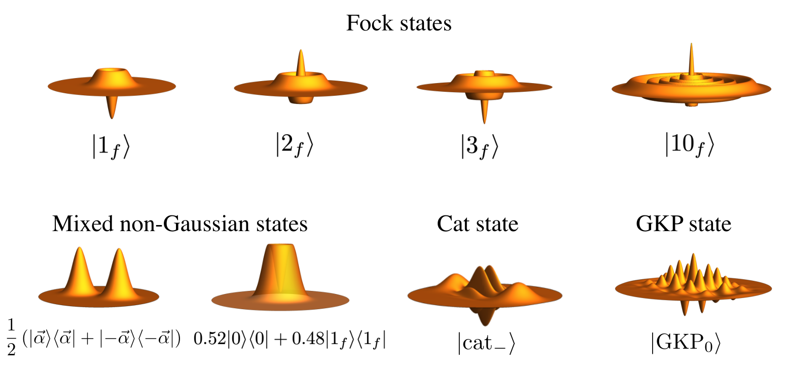
A first important class of non-Gaussian states are Fock states, generated by acting with creation operators on the vacuum state
| (117) |
which is a state of photons in mode . These states are inherently single-mode, even though they can be embedded in a much larger multimode state space. The Wigner function for such states is commonly found in quantum optics textbooks, but deriving it using (38) is a good exercise. Here we simply state the result:
| (118) |
In the most general sense, we write as the projector of on the phase space of mode , but it is most practical to use the coordinate representation where and to describe the two-dimensional phase space associated with mode .
Multimode Fock states can be obtained by acting on the vacuum with different creation operators in different modes. Even though these different modes do not necessarily have to be orthogonal Walschaers 2020, we here focus on the case where they are. For example, in -mode system, we can chose a basis of the phase space and define multimode Fock states as
| (119) |
where the th mode in the basis contains photons. Note that for we have a vacuum mode. For the Wigner function, this implies
| (120) |
Here we have used that the phase space point can be expressed as , where is the phase space coordinate within the subspace spanned by and . We can note , such that we find the coordinate representation in the chosen basis of phase space.
Non-Gaussian states do not necessarily have to be pure, they can also come in the form of statistical mixtures. The most basic example of such as state is a non-Gaussian mixture of Gaussian states. As a simple example, let is consider a mixture of two coherent states
| (121) |
Even though this is a highly classical state, it is still non-Gaussian as clearly seen from its Wigner function
| (122) |
Another important example of a non-Gaussian mixed state is
| (123) |
In the mode , the Wigner function of the state behaves as
| (124) |
This Wigner function reaches negative values as long as and subsequently becomes positive. Nevertheless, it will remain non-Gaussian until . As we will see in Subsection III.3, even when the Wigner function is positive, it is not always possible to describe this state as a mixture of Gaussian states.
Generally speaking, non-Gaussian states can come in a wide variety of shapes which can be much more exotic than the examples discussed above. A popular class of Gaussian states is obtained by taking coherent superpositions of Gaussian states. As we will see in Section VII, there has been a strong experimental focus on two specific types of such states: Schrödinger’s cat states Yurke and Stoler 1986 and Gottesman-Kitaev-Preskill (GKP) states Gottesman et al. 2001. The former are obtained by coherently superposing two coherent states, and often are split in even and odd cat states:
| (125) |
where is the normalisation coefficient which depends on the displacement . The latter is often referred to as “the size of the cat”. The Wigner function of these states resembles that of (122) but has an additional interference term
| (126) |
The appearance of these interference terms creates several regions in phase space where the Wigner function attains negative values. The term “Schrödinger’s cat state” has historically grown from the idea that coherent states describe classical electromagnetic fields and can thus be considered “macroscopic”, in particular for large values of . However, one should honestly admit that they fail to capture an important point of Schrödinger’s thought experiment Schrödinger 1935a: the entanglement with a microscopic quantum system (i.e., the decay event that triggers the smashing of the vial of poison). Nevertheless, the term “cat state” has established itself firmly in the CV jargon, and now also lies at the basis of derived concepts such “cat codes” for error correction Cochrane et al. 1999; Leghtas et al. 2013.
Finally, there are the GKP states. In their idealised form, they rely on eigenvectors of the quadrature operators (sometimes also known as infinitely squeezed states). To keep notation simple, we will restrict to the single mode with quadrature operators and . The eigenvectors of these operators are then formally written as
| (127) |
Furthermore, we have the relations , and . GKP states are constructed by considering a grid of such states to create a qubit, by identifying the two following GKP vectors:
| (128) | ||||
| (129) |
Clearly, these states are not normalisable and not physical as they would require infinite energy to be created. Thus, it is common to construct approximate GKP states, by replacing the states with displaced squeezed states, and by truncating the summation by adding a Gaussian envelope:
| (130) | ||||
| (131) |
here are normalisation constants and is a single-mode squeezed vacuum, which implies that its Wigner function is given by (85) with and for . To get a good GKP state for quantum error correction, we generally need that . The Wigner function of an ideal GKP state is a grid of delta functions, which again highlights that it is a non-physical state. The more realistic states and have well-defined Wigner functions, even though they are not very insightful to write down explicitly. In Fig. 2, we plot an example that was calculated numerically by taking into account only the first few terms around in the sum.
GKP states may seem a little artificial at first glance, but they have we developed with a very clear purpose: to encode a qubit in a harmonic oscillator Gottesman et al. 2001. This encoding implies a notion of fault-tolerance as these states are designed to be very efficient at correcting displacement errors. The more realistic incarnations of these states (130) are therefore often proposed as candidates for encoding the information in CV quantum computation protocols Menicucci 2014. Furthermore, it was shown that these states can also be used as the sole non-Gaussian resource to implement a CV quantum computer Baragiola et al. 2019
Once we progress into the realm of multimode states, the class of non-Gaussian states becomes even more vast. In Subsection IV.2.2, we will present a dedicated introduction to multimode photon-subtracted states, which is a useful state general concepts in this Tutorial. Furthermore, these states have a particular importance in CV quantum optics experiments. As a final example, we introduce another class of multimode non-Gaussian states, which have been highly relevant for quantum metrology: N00N states Sanders 1989; Boto et al. 2000; Lee et al. 2002. Even though these states very useful for quantum sensing with optical setups, the general idea that underlies these states was first introduced for fermions Yurke 1986 in an attempt to mimic the advantage that is provided by squeezing in optics.
N00N states are two-mode entangled states defined in a pair of orthogonal modes and . The state contains exactly photons, and is a superposition of a state with all photons being mode and a state with all photons in mode :
| (132) |
Here we recall that the state can be trivially embedded to the full multimode space by adding vacuum in all other modes. We will study these states in more detail for in our discussion of the Hong-Ou-Mandel effect surrounding Eq. (165). However, here we highlight already that the Wigner function of is not simply the sum of Wigner functions of the form (118). The entanglement will create additional interference terms, just like we saw in (126). In the present case, these interferences are genuinely multimode, and thus related to quantum correlations.
Experimentally, these states have been created and analysed using a DV approach Israel et al. 2012. As we highlighted in Subsection II.3, the distinction between DV and CV is somewhat subtle and mainly depends on what is measured. Because N00N states are built from Fock states and have a well-defined total photon number, they are most natural to analyse using photon-number resolving detectors.
III.3 Quantum Non-Gaussianity
Non-Gaussian states come in a wide variety, which means also that some of them are more exotic than others. Non-Gaussian states that are of limited interest, are those which are convex combinations of Gaussian states. Gaussian states do not form a convex set, after all, we can immediately see that, e.g., is not a Gaussian function even though it is a convex combination of Gaussian states.
The fact that the set of non-Gaussian states contains mixtures of Gaussian states may lead one to suspect that any mixed state with a positive Wigner function can be written as a well-chosen mixture of Gaussian states. After all, Gaussian states are the only pure states with positive Wigner functions. This intuition turns out to be false Filip and Mišta 2011, which means that the set of states with a non-positive Wigner function is not the same as the set of states that lie outside of the convex hull of Gaussian states . More formally, let us define
| (133) |
where is some arbitrary way of labelling Gaussian states and is a probability distribution on these labels. Note that (103) tells us that we can generate all Gaussian states by taking convex combinations of displaced squeezed states, and thus we can limit ourselves to in the definition of .
Any quantum state that is not contained in the convex hull of Gaussian states, i.e., , is referred to as a “quantum non-Gaussian” state. The intuition behind this terminology is that Gaussian pure states are less quantum than non-Gaussian pure states that boast a non-positive Wigner function. A mixed state that is quantum non-Gaussian may have a positive Wigner function, but it cannot be created without adding states with non-positive Wigner functions into the pure-state decomposition. Hence, these states are more quantum than the states that are in the convex hull of Gaussian states .
Next, one may wonder how to differentiate between states that are quantum non-Gaussian and states which are in the convex hull . Throughout the last decade, many methods have been developed to answer this question. We start by introducing the main idea of Ref. Genoni et al. 2013 because it is based on the Wigner function. The key idea is that Gaussian distributions have tails, which means that we can take an arbitrary pure Gaussian state , and evaluate the Wigner function at to origin of phase space:
| (134) |
Clearly, when , we do find that . This limit essentially corresponds to a system with infinite energy. It is thus natural to try to bound the value of the Wigner function in the origin by a function that depends on the energy of the state. For an arbitrary pure Gaussian state, we find that
| (135) |
Using the properties of the operator norm, we write , where is a symplectic orthogonal transformation. Furthermore, we note that . It is then useful to explicitly write the coordinate representation of the vector , such that
| (136) | ||||
| (137) |
At the same time, we expand
| (138) |
and with a little algebra we can show that
| (139) |
such that
| (140) |
This means that the value of the Wigner function of a pure Gaussian state in the origin of phase space is bounded from below by a function of the average number of particles . However, it is not obvious that we can extend this bound to arbitrary mixtures of Gaussian states. Let us assume that , then the Wigner function in the origin is given by
| (141) |
where we saw that is the value of a pure Gaussian state’s Wigner function in the origin and is some arbitrary label for the Gaussian states in the mixture. Therefore we can bound the states in the convex combination
| (142) |
where we introduce a probability distribution on the average particle numbers of the pure Gaussian states in the mixture. The overall average number of particles in the state is then given by . The final element that we require is the fact that is a convex function, such that we can apply Jensen’s inequality to find that
| (143) |
This means that we can simply use the total energy of the state to construct a witness for quantum non-Gaussianity. This clearly shows that there are quantum non-Gaussian states with positive Wigner functions. An explicit example can be constructed by tuning the in the state to (where we use that is also the average particle number in this particular state).
Nevertheless, there are many quantum non-Gaussian states that do not violate inequality (143). After all, why would the origin of phase space be the most interesting point? A first solution is provided in Genoni et al. 2013, where it is argued that
| (144) |
for all Gaussian channels that act on the Wigner function of as . Recall that the action of a Gaussian channel was defined in (102). The quantity then denotes the average number of particles in the state . Further generalisations of this scheme have been worked out in Hughes et al. 2014. Moreover, Ref. Park et al. 2015 has considered combinations of the value of the Wigner function in several points to reach better witnesses for quantum non-Gaussianity. Further progress has been made by identifying observables that are more easily measurable with typical CV techniques Happ et al. 2018. Others have considered other phase-space representations of the state to identify witnesses of quantum non-Gaussianity Kühn and Vogel 2018; Bohmann et al. 2020.
Quantum non-Gaussianity has been investigated with a wide range of tools. In this Tutorial we have limited ourselves to phase space methods in the spirit of the CV approach. However, there is also a significant body of work on quantum non-Gaussianity using techniques that are more typical in DV quantum optics. The earliest works on the subject used photon-statistics to distinguish quantum non-Gaussian states from convex mixtures of Gaussian states Filip and Mišta 2011. This research line has been continued in recent years to uncover new aspects of quantum non-Gaussian states, such as the “non-Gaussian depth” Straka et al. 2014 and techniques to differentiate different types of multi-photon states Straka et al. 2018. Ultimately, these photon-counting techniques were extended to develop a whole hierarchy of quantum non-Gaussian states Lachman et al. 2019. These ideas have been further formalised and generalised through the notion of the “stellar rank” of a quantum state.
III.4 Stellar Rank
An interesting starting point to introduce the stellar representation is the method Lütkenhaus and Barnett 1995 to prove Hudson’s theorem. We recall the definition
| (114) |
of what we will henceforth refer to as the stellar function. To avoid technical complications, let us now restrict ourselves to single-mode systems such that the optical phase space is . Note that, in a single-mode system, there is only one creation operator with associated annihilation operators . We can then follow Chabaud et al. 2020 to introduce the stellar representation of single-mode quantum states. Note that some similar ideas are also present in other works Gagatsos and Guha 2019.
First, we develop the stellar representation for pure states, which will then be used to generalise the framework to mixed states in (148). We use the definition of the displacement operator to show that
| (145) |
which immediately implies that the stellar representation is unique. In other words, if it follows that up to a phase. In our proof of Hudson’s theorem, we have already highlighted that satisfies the property (116) which means that it is an entire function with growth order . Because in this single-mode setting can be interpreted as a function of a single complex variable, the Hadamard-Weierstrass theorem implies that can be fully represented by its zeros (one can consider this as a generalisation of the fundamental theorem of calculus). This thus implies that a single-mode state is completely determined by the zeros of the , and thus by the zeros of the Q-function in eq. (115).
It is thus natural to use these zeros in order to classify pure single-mode quantum states and thus the stellar rank is introduced. Ultimately, the stellar rank is simply given by the number of zeros of or alternatively the number of zeros of the Q-function. Because in practice zeros may coincide, one should also consider the multiplicity of the zeros. We thus define the stellar rank of as the number of zeros of counted with multiplicity. Alternatively one may count the zeros of the Q-function with multiplicity and divide by two.
The fact that a state is fully characterised by its stellar representation can be made more explicit by considering the roots of the Q-function which represents (note that we use (44) to interchange between phase-space representation and complex Hilbert space representation). The single-mode state can then be used to express
| (146) |
where is a pure Gaussian state and a normalisation constant. We can then use the stellar rank to induce some further structure in the set of states by defining
| (147) |
that groups all states of stellar rank . Note that the Hadamard-Weierstrass theorem also considers functions with an infinite amount of zeros and the case is thus mathematically well-defined. It turns out that this case is not just a pathological limit. An evaluation of the Q-function shows that Gottesman-Kitaev-Preskill states and Schrödinger cat states inhabit the set .
Clearly, all that was introduced so far only works for pure states. We can naturally extend this result via a convex roof construction, by defining
| (148) |
where the infimum is considered of all probability distributions on the set of pure states that lead to . In words, there are many ways to decompose the state in pure states and we consider all of them. For each decomposition, we define the stellar rank as the highest rank of the states in the decomposition. Then we minimize these values over all possible decompositions to arrive at the stellar rank of .
Convex roof constructions are commonly used to treat mixed states as they are easy and natural to formally define. However, they are often much harder to calculate in practice. This is where the stellar representation unveils its most remarkable property: stellar robustness. To formalise this idea, Chabaud et al. 2020 introduced the robustness as the trace distance between the state and the nearest possible state of lower stellar rank.
| (149) |
And it can be shown that
| (150) |
where is the fidelity of with target state . Remarkably, it can be shown that when Chabaud et al. 2020. This means that any state that is sufficiently close to a pure state of is also of rank or higher.
The idea of stellar robustness can be generalised Chabaud et al. 2021a by introducing -robustness. For any , we define
| (151) |
and show subsequently that
| (152) |
The -robustness can thus be interpreted as the nearest distance from a state at which we can find any state of stellar rank , provided . Beyond showing that is non-zero when is of finite stellar rank, Ref. Chabaud et al. 2021a also provides an explicit method to calculate . Thus, for whichever state is available in an experiment one can attempt to find a pure target state for which to prove that is at least of stellar rank .
We note that for pure states implies that the state is Gaussian (this is essentially what is proven in Hudson’s theorem). From the definition (148) we can then deduce that
| (153) |
where denotes, again, the convex hull of Gaussian states. On the other hand, states for which cannot be written as a mixture of Gaussian states and are thus quantum non-Gaussian.
This idea can be extended by using the stellar -robustness (152) as a witness of quantum non-Gaussianity. When we want to check whether is quantum non-Gaussian, it suffices to find a pure target state such that is closer to than the -robustness . More formally written, whenever a pure state exists with the following property:
| (154) |
and is quantum non-Gaussian. This may seem like a complicated challenge, but for a single-photon state we find that Chabaud et al. 2021a. This means that any state which has a fidelity of more than with respect to a Fock state is quantum non-Gaussian. This idea can be extended to higher stellar ranks: whenever we find a target state such that the state is at least of stellar rank . Note that the fidelity of an experimentally generated state with any pure target state can be calculated from double homodyne measurements on Chabaud et al. 2021a. There is no need to experimentally create the pure state , the latter is just theoretical input needed to analyse the data.
Obviously, the stellar rank imposes a lot of additional structure on the state space. It rigorously orders all states that can be achieved by combining a finite number of creation operators and Gaussian transformations. The creation operator serves as a tool to increase the stellar rank by one and the stellar rank actually corresponds to the minimal number of times the creation operator must be applied to obtain the state, together with Gaussian operations. The stellar rank remains unchanged under Gaussian unitary transformations, which makes sense for a measure of the non-Gaussian character of the state, and thus it falls within the set of intrinsic properties of a state as discussed in Subsection II.3. Furthermore, the class of states with infinite stellar rank can be understood as the set that contains the most exotic states. However, it is lonely at the top as it can be shown that for states of infinite rank. This means that we can find states of finite stellar rank arbitrarily close to a state of infinite stellar rank. As stressed in Chabaud et al. 2020, this implies that finite rank states are dense in the full Fock space and any state of infinite-rank can be arbitrarily well approximated by finite rank states. Whereas a finite stellar rank of any experimental state can be certified by achieving a sufficiently high fidelity to a target state to fall within the range given by its -robustness , a similar procedure is impossible for infinite stellar ranks. This means, in practice, that genuinely infinite-rank states are impossible to certify in experiments because one never achieves perfect fidelity. Nevertheless, different states of infinite rank may differ significantly in the values for .
Many of the results on stellar rank rely on the Hadamard-Weierstrass theorem that allows to uniquely factorise as a Gaussian and a polynomial, where the roots of the polynomial are the roots of and thus also the roots of the Q-function. Sadly, this theorem cannot be straightforwardly generalised to a multimode setting, which is known in mathematics as Cousin’s second problem Lelong and Gruman 1986. Notable progress was made in Chabaud et al. 2021b where one studies multimode stellar functions which are polynomials and it was shown that there is no straightforward generalisation of (146).
III.5 Wigner Negativity
Hudson’s theorem shows us that all pure non-Gaussian states have non-positive Wigner functions, which sets them apart from normal probability distributions of phase space. For mixed states, this no longer holds and thus we spent the previous two sections developing methods to characterise the non-Gaussian features of these states. Whether it is through quantum non-Gaussianity or the more refined stellar rank, these methods focus on characterising the non-Gaussian resources that are required to generate a certain state. In this subsection, we change the perspective and focus rather on negative values of the Wigner function (“Wigner negativity” in short) as a resource of interest.
Wigner negativity has the advantage of being a clear quantum feature, it reflects that different quadratures in the same mode cannot be jointly measured and thus goes hand in hand with the principle of complementarity. More formally, it has even been connected to the principle of quantum contextuality Spekkens 2008. Indeed, in Section VI we will elaborate on the fact that Wigner negativity is a necessary resource for reaching a quantum advantage, i.e., performing a task that cannot be efficiently simulated by a classical computer. However, the idea of using Wigner negativity as a signature of non-classicality was already around before it was connected to a quantum computational advantage. An important step to formalise this idea was the introduction of a measure for Wigner negativity Kenfack and Życzkowski 2004, which lies at the basis of recent resource theories of Wigner negativity Takagi and Zhuang 2018; Albarelli et al. 2018.
A priori, there are several natural measures than can be used for Wigner negativity. It is therefore useful to consider some desirable properties that are required for a measure of Wigner negativity. First of all, we want the measure to be zero if and only if the Wigner function is positive. It seems natural to demand that, furthermore, Wigner negativity remains unchanged under Gaussian unitary transformations. It is then tempting to simply consider the absolute value of the lowest possible value of the Wigner function, but this would have some unnatural outcomes. It would mean that a single photon state would have more Wigner negativity than a two photon state. We thus need to look for a different measure.
The starting point of Kenfack and Życzkowski 2004 is that the normalisation of the Wigner function implies that
| (155) |
and that the inequality is strict whenever there is Wigner negativity. Furthermore, Liouville’s theorem implies that integrals over phase space are unchanged by Gaussian transformations. A first possible way of measuring Wigner negativity is through the negativity volume
| (156) |
This measure has the major advantage of being convex due to the triangle inequality, which means that for we find that
| (157) |
However, this measure is not additive, i.e., . To circumvent this shortcoming, another measure for Wigner negativity has been introduced Veitch et al. 2014; Takagi and Zhuang 2018; Albarelli et al. 2018:
| (158) |
Clearly, making this measure additive. However, the introduction of the logarithm destroys the convexity of the measure. Note that the two measures are closely related by . Thus when , we also find that .
The single-mode examples that are considered in Ref. Kenfack and Życzkowski 2004 lead to some interesting observations. First of all, they show that for Fock states Wigner negativity increases with the photon number. Furthermore, they show that for Schrödinger cat states the integral is bounded from above by a value smaller than the Wigner negativity of a two-photon state. Even though Fock states of increasing stellar rank have increasing Wigner negativity, there is no clear relation between stellar rank and Wigner negativity for more general classes of states. For example, Schrödinger cat states are of infinite stellar rank, suggesting that they are in this regard the most exotic states, but they only manifest a limited amount of Wigner negativity.
As a case study, let us briefly concentrate on the Wigner negativity of Fock states (117). One can now evaluate the Wigner negativity of such states to find that
| (159) | ||||
| (160) | ||||
| (161) |
which shows that the negativity does not simply increase linearly with the number of photons even for the additive measure . However, let us now look at a multimode -photon state where each photon occupies a different mode, i.e., a Fock state generated by creation operators in with for all ,
| (162) |
The Wigner function for this state can be shown to be (showing this based on (38) is again a good exercise)
| (163) |
Either by explicitly using the expression of the Wigner function, or by using the additivity property, we find that
| (164) |
Numerically, we can show that and thus we can generally conclude that photons in different modes hold more Wigner negativity than photons in the same mode.
Let us now concentrate on the case where . We showed that two photons in different modes are more Wigner negative than two photons in the same mode, and now we will combine this finding with the idea that Wigner negativity remains unchanged under Gaussian transformations. A particularly simple Gaussian transformation is a balanced beam splitter, which ultimately just implements a change in mode basis that we describe by an orthonormal transformation . When we mix two photons, prepared in orthogonal modes and by such a balanced beamsplitter, we will see the Hong-Ou-Mandel effect in action (more details can be found in Walschaers 2020 where a similar notation is used):
| (165) |
where and are the input and output modes of the beam splitter, respectively. The Hong-Ou-Mandel output state is thus a superposition of two photons in mode and two photons in mode . We can now use the simple fact that Wigner-negativity is unchanged under Gaussian unitary transformations to show that
| (166) |
this then also implies that . At first sight, this is somewhat of a peculiar finding: by taking a superposition of two states with the same Wigner negativity one finds a state with a higher Wigner negativity.
An explicit look at the Wigner function of the Hong-Ou-Mandel state provides some insight. We find that this Wigner function can be written as (yet again a good exercise to show this explicitly)
| (167) |
where is the contribution to the Wigner function that contains all the interference terms that are induced by the superposition. We can calculate that
| (168) |
and thus, by additionally applying the triangle inequality, we can understand that the additional negativity in the Hong-Ou-Mandel state is due to the term .
In the Hong-Ou-Mandel effect, it is common to talk about interference between particles, but in a more general CV language this interference will be equivalent to some form of entanglement which is exactly described by the Wigner function contribution . In other words, the superposition between and has more Wigner negativity than each of its two constituents because it creates entanglement between the modes and . This is a first indication that there is a connection between quantum correlations and non-Gaussian features of the Wigner function. We will explore this connection in further detail in Section V.
Even though Wigner negativity is an important non-Gaussian feature, it is often hard to witness Chabaud et al. 2021c. The most common experimental technique is homodyne tomography Ourjoumtsev et al. 2006a to fully reconstruct the quantum state. These methods come with the inconvenience that it is hard to set good error bars. Techniques to circumvent the need for a full tomography have been developed based on homodyne Mari et al. 2011 and double-homodyne (or heterodyne) measurements Chabaud et al. 2021a; Chabaud et al. 2021c. These methods come with the advantage of permitting to put a degree of confidence on the proclaimed Wigner negativity.
IV Creating Non-Gaussian States
In Section III we have discussed the many ways of characterising non-Gaussian quantum states and their properties. In this section, we explore the different theoretical frameworks for creating these states. An overview of some important experimental advances to put these theoretical techniques into practice is left for Section VII.
Gaussian quantum states can in some sense be understood as naturally occurring states. The foundational work of Planck that lies at the basis of all of quantum mechanics provides a first description of the thermal states of light that describe black body radiation. In a more modern language, we refer to this as the thermal states of an ensemble of quantum harmonic oscillators or a free bosonic field. It has long been understood that these states are Gaussian Araki and Woods 1963; Robinson 1965; Verbeure 2011. Creating this kind of Gaussian states of light is thus literally as simple as switching on a light bulb.
When we turn towards more sophisticated light sources such as lasers, we can encounter coherent light that is described by coherent states Glauber 1963; Sudarshan 1963. Generating squeezed light becomes much harder and typically requires nonlinear optics Loudon and Knight 1987. Nevertheless, pumping a nonlinear crystal with a coherent pump generally suffices to deterministically create a squeezed state Wu et al. 1986. Recall from the end of subsection II.4 that from a theoretical point of view all these pure Gaussian states can be created by applying Gaussian unitary transformation to the vacuum state.
From an experimental point of view, the creation of non-Gaussian states is much harder than the creation of their Gaussian counterparts. Nevertheless, we start by introducing an ideal theoretical approach that is not too different from Gaussian states. In essence, it suffices to apply a non-Gaussian unitary operation to the state to create a non-Gaussian state. In Subsection IV.1 we dig deeper into the desired structure of such non-Gaussian unitary transformations that would in principle allow for the deterministic generation of non-Gaussian quantum states. In experiments (in particular those in optics) such non-Gaussian unitary transformations are hard to come by, which is why one very often uses different preparation schemes. In Subsection IV.2, we provide a general introduction into the conditional preparation of non-Gaussian quantum states, where one measures part of the system and conditions on a certain measurement outcome. This process projects the remainder of the system into a new non-Gaussian state.
IV.1 Deterministic methods
To introduce some further structure in the sets of Gaussian and non-Gaussian unitary transformations, it is useful to take a quantum computation approach that is inspired by DiVincenzo 1995; Lloyd and Braunstein 1999. The central idea of this work is that Gaussian unitary transformations are always generated by “Hamiltonians” that are at most quadratic in the quadrature operators (or equivalently in the creation and annihilation operators). Let us denote that as
| (169) |
where the polynomials are generated by combining terms of the types , , and . A remarkable property of these three types of observables is that they are closed under the action of a commutator. Indeed, using the canonical commutation relation (29) and the general properties of commutators, we can show that
| (170) | ||||
| (171) | ||||
| (172) |
Thus, we can use the Baker-Campbell-Hausdorff formula to show that the combination of two Gaussian unitaries is again a Gaussian unitary.
This notion lies at the basis of universal gate sets in the CV approach. Using typical techniques from Lie groups, we can look for a minimal set of Gaussian unitaries than can be combined to generate all possible Gaussian unitary transformations. Generally, such a set is clearly not unique, but there are some natural choices. For example, we previously saw that a Gaussian unitary transformation is a combination of displacement operations and symplectic transformations. Furthermore, the Bloch-Messiah decomposition (95) shows us that any symplectic transformation can be decomposed into a combination of multimode interferometers and single-mode squeezing. In turn, interferometers can be decomposed as a combination of beamsplitters and phase shifters Reck et al. 1994. Indeed, we can choose the set of Gaussian gates to be
| (173) | ||||
| (174) | ||||
| (175) | ||||
| (176) |
where we note that are not normalised and . These unitary operators describe a displacement, a squeezer, a phase shifter, and a beamsplitter, respectively. We note that all these operations act on a single modes, except for the beamsplitter which connects a pair of modes. These transformations are referred to as a Gaussian gate set; when we can implement all these gates in all the modes of some mode basis, we can generate any multimode Gaussian transformation, and thus any Gaussian state.
To generate non-Gaussian unitary transformations and thus non-Gaussian states, we need to add more unitary gates to the Gaussian gate set. The relevant question is thus how many gates one should add and which gates are the best choices. The answer to the first question is surprising: one needs to add just one single gate Menicucci et al. 2006. The argument is simple, when we consider the operators , we find that
| (177) |
With the canonical commutation relations we can show that , which can be inserted in (177) to obtain
| (178) |
This calculation thus shows that commutation with the operators increases the order of the quadrature operators. Thus, with the quadratic Hamiltonians to generate all operations that conserve the order of polynomials of quadrature operators and to increase the order of the polynomial by one, we can ultimately generate the full algebra of observables. On the level of unitary gates, this implies that a full universal gate set is given by
| (179) | ||||
| (180) |
In other words, combining sufficiently many of these gates allows us to built any arbitrary unitary transformation generated by a Hamiltonian which is polynomial in the quadrature operators.
The non-Gaussian gate is known as the cubic phase gate. The argument above shows that any experiment that can implement Gaussian transformations and a cubic phase gate can in principle generate any arbitrary non-Gaussian state. Even though many protocols have been proposed to experimentally realise a cubic phase gate Gu et al. 2009; Marek et al. 2011; Marshall et al. 2015; Miyata et al. 2016; Yanagimoto et al. 2020, any convincing implementations have yet to be demonstrated. One of the key problems is that experimental imperfections and finite squeezing are detrimental for the most commonly proposed methods Arzani et al. 2017.
In principle, there is no particular reason to limit our attention to cubic phase gates. Already in the very first work on the subject it is argued that essentially any Hamiltonian of a higher than quadratic order can be used a a generator Lloyd and Braunstein 1999. Thus, optical processes that performs photon triplet generation can also be used as a non-Gaussian gate, which can even be converted into the cubic phase gate PRXQuantum.2.010327. This requires well-controlled high nonlinearities which are generally only achieved by using exotic nonlinear crystals or well-controlled individual atoms. Handling such setups with a sufficient degree of control to actually implement a quantum gate is extremely challenging.
Other CV systems are more appropriate for the implementation of non-Gaussian unitary transformations. In particular the systems used in circuit-QED have such non-Gaussian contributions in their Hamiltonians Vion et al. 2002; Devoret and Schoelkopf 2013 which suggests that they may be more capable of deterministically generating non-Gaussian states than their optical counterparts. Still, the characterisation, detection, and control of such states is expected to be challenging. Recently, some important progress was made by demonstrating triplet-generation in these systems Chang et al. 2020.
IV.2 Conditional methods
The experimental difficulties that are encountered when trying to implement non-Gaussian unitary transformations can be circumvented by abandoning the demand of unitarity. This implies that we no longer consider operations that can be implemented deterministically, but rather resort to what can be broadly referred to as conditional operations. This idea was formalised by Kraus when characterising the most general ways of manipulating quantum states Kraus 1971.
In the most general sense, we can implement a conditional operation by taking a set of linear operators on Fock space and acting on the state in the following way
| (181) |
This formalism is typically implemented by performing some form of generalised measurement on the state Hol 2001. When is a deterministically generated Gaussian state, the action of a well-chosen set of operators can turn it into a non-Gaussian state. In optics, two of the most well-known examples of this technique are single-photon addition and subtraction. In both cases, there is only a single operator . For photon addition, we implement , whereas photon subtraction requires the realisation of a case where .
In many physical setups, and in particular in optics, the problem is that measurements are destructive and a measurement effectively removes the measured mode from the system. Therefore, it is common to prepare large multimode Gaussian states of which a subset of modes is measured in order to conditionally prepare a non-Gaussian state in the remaining modes. We now introduce a general framework to describe the non-Gaussian Wigner functions that are created accordingly Walschaers et al. 2020.
IV.2.1 General framework
First of all, let us consider a general multimode phase space and separate it into two subsystems, i.e., , where we will perform some generalised measurement on the modes and leave the remaining modes untouched. This introduces a general structure in the points of phase space , which can now be written as with and . The general procedure is schematically outlined in Fig. 3 and we will present the details step by step.
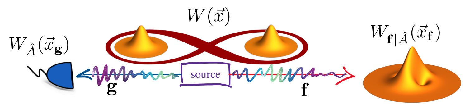
Any state on this system then comes with a Wigner function that is defined on the global phase space. This state can be reduced to one of the two subsystems by tracing out the other subsystem, which can be described on the level of the Wigner function by the following integrals:
| (182) | |||
| (183) |
When the state is Gaussian and the Wigner function is given by (85), the structure of the phase space is reflected in the mean field vector and in the covariance matrix :
| (184) | ||||
| (185) |
with . The matrices and describe all the variances and correlations of the modes within and , respectively. In addition, the submatrix contains all the correlations between the modes in the different subspaces, which will be important for conditional state preparation. One can show that for such Gaussian states, the reduced states are also Gaussian, for the modes in given by
| (186) |
and analogously for the modes in . As Gaussian states are the states that are least challenging to produce, they form the starting point of the conditional state preparation scheme.
As a next step, we must implement some form of operation on the modes that correspond to the phase space . To do so, we consider the action of a general POVM element that corresponds to a specific measurement outcome. We can then obtain a conditional state via
| (187) |
The partial trace only runs over the modes in because the other modes are left untouched. The denominator renormalises the state and gives the probability of actually obtaining the measurement result that corresponds to . In an actual experiment, this operation is implemented by many repeated measurements of the modes in and corresponds to a specific detector output of these measurements. The non-measured part of the state is only used when the detector indicates this specific output, otherwise it is simply discarded. This conditional selection of the state significantly changes the properties of the state in a way that is strongly influenced by .
As we described in (42), the operator comes with an associated phase-space representation which can be used to formally describe the phase-space representation of :
| (188) |
There is a more practical way of expressing this Wigner function by exploiting the fact that the initial multimode Wigner function is positive and therefore describes a well-defined probability distribution on phase space. This implies that the conditional probability distribution
| (189) |
is also a well-defined probability distribution, which is obtained when we fix one point in phase space and look at the probability distribution for the remaining modes in . We can then use this conditional probability distribution to write , which can be inserted in (188) to find
| (190) |
where we define
| (191) | ||||
| (192) |
The quantity is simply the expectation value of the observable in the state . on the other hand, is the expectation value of the function where is distributed according to the distribution , which makes a function of the selected phase space point . However, even though is a well-defined probability distribution on phase space, it does not necessarily correspond to a quantum state. Indeed, may violate the Heisenberg inequality which will be of vital importance in Section V as it is narrowly connected to quantum steering.
In the specific case where is Gaussian, we find that is also a Gaussian probability distribution, given by
| (193) |
Using the notation of (185), we express its covariance matrix
| (194) |
and mean field vector
| (195) |
The covariance matrix is known in the mathematics literature Horn and Johnson 2017 as the Schur complement of . The Schur complement is interesting properties, for example, is a positive matrix if and only if the same holds for the Schur complement . This immediately implies that the Gaussian probability distribution in (193) is well-defined. Furthermore, the Schur complement also plays an important role in the theory of Gaussian quantum correlations Lami et al. 2018. It should be noted that does not actually depend on the chosen value for . Thus, the conditional expectation value only depends on the phase space point through the displacement . This is a particular feature of Gaussian states.
Finally, remark that the derivation of (190) holds true for all initial states with a positive Wigner function. Whenever the initial multimode Wigner function is positive, it follows that is also positive. Furthermore, given that is the quantum expectation value of a positive semi-definite operator it clearly also is a positive quantity. Hence, Wigner negativity is entirely contained with . The fact that can take negative values is exactly due to not being the Wigner function of a quantum state. Furthermore, (192) teaches us that the conditionally generated Wigner function can only achieve negative value when is non-positive.
Thus, in order to conditionally prepare a state with Wigner negativity, one faces strict requirements, on both the POVM element that is conditioned upon and on the conditional probability distribution that is obtained from the initial multimode state. We will discuss this point in greater detail in Section V.2. For a more experimentally-inclined perspective on the production of non-Gaussian states, we refer to Lvovsky et al. 2020.
Before we move on to consider photon subtraction as an example of conditional creation of non-Gaussian states, let us take a moment the opposite process: Gaussification. The authors of Browne et al. 2003 consider several copies of an initial non-Gaussian state which are mixed through linear optics and subsequently some output modes are measured with on-off detectors. The conditioning is done of the events where no photons are detected, and such that we can interpret as a projector in vacuum. By repeating several iterations of this scheme (assuming many successful conditioning events), the initial non-Gaussian state is converted into a Gaussian state. The Gaussification process thus relies on starting from a non-Gaussian state and conditioning by projecting on a Gaussian state: the vacuum. This point of view nicely complements our approach to create non-Gaussian states.
IV.2.2 An example: photon subtraction
Single-photon subtracted states are theoretically obtained by acting with an annihilation operator on the state. Their density matrices are given by
| (196) |
if the photon is subtracted in one specific mode . In practice Wenger et al. 2004; Ourjoumtsev et al. 2006a; Zavatta et al. 2008, we can implement this operation on the state through a mode-selective beamsplitter , that couples the mode to an auxiliary mode which is prepared in a vacuum state. We thus describe the action of the beamsplitter on the system of interest and the auxiliary mode as . As a next step, we mount a photon-detector on one of the output modes of the beamsplitter and condition on events where the detectors count a single photon. Thus, we generate the state
| (197) |
The reader can now recognise (187). As a next step, we assume that the beamsplitter is transmitting nearly all the incoming light, such that . We can then approximate . Then, when we insert this approximation in the expression for , we find that only the terms survive such that
| (198) |
A much more detailed analysis of multimode photon subtraction with imperfect mode-selectivity can be found in Averchenko et al. 2016. We note that through this approach, photon subtraction can be understood as a weak measurement of the number of photons Wiseman and Milburn 2009.
We can now derive the Wigner function of a single-photon-subtracted state through (193) by following the idea of (197). We initially start from a Gaussian state with covariance matrix and one auxiliary mode that is prepared in the vacuum
| (199) |
We then implement a mode-selective beamsplitter that mixes one specific mode with the auxiliary vacuum mode, following the scheme outlined in Fig. 4. An effective way to describe such a transformation is by designing a new mode basis , which has as one of the modes in the mode basis. We complete the basis with complementary modes , such that the modes basis of phase space is given by . Thus, we can perform such a basis change as
| (200) |
where the matrix of basis change is given by
| (201) |
It is now instructive to explicitly write the rows and columns corresponding to mode :
| (202) |
Note that is the matrix that describes the initial state covariances of mode , while is the that describes all the covariances in the complementary modes. The rectangular matrices and contain all the correlations between the mode and the complementary modes in the basis. Now, we mix the mode and the auxiliary vacuum mode on a beam splitter. This beamsplitter is implemented by the transformation
| (203) |
where is given by
| (204) |
As a final step, we change the basis back to the original basis, such that the final state’s covariance matrix becomes
| (205) |
We can now rewrite this entire transformation such that the matrix in (185) is given by
| (206) |
with
| (207) |
We introduce the matrix which implements the mode-selectivity of the beamsplitter in mode and is defined as
| (208) |
Hence, we can simply use as a mode-selective beamsplitter that mixes one specific mode of a multimode state with the auxiliary mode. We should highlight that ultimately turns out to be independent of the complementary modes . This means that the finer details of the interferometer are not important for the final , the key point is that changes towards a mode basis in which and are basis vectors of the phase space.

For the particular case of photon subtraction, we consider a very weak beamsplitter, such that we consider the limit . In this case, we can express the conditional mean field (195) and covariance matrix (194) of the auxiliary mode by
| (209) | ||||
| (210) | ||||
where we introduce the matrices , , and as well as the vector . We can then use these quantities to evaluate that
| (211) | ||||
As a next step, we must choose a POVM element to measure. In the case of photon subtraction, we mount a photon counter on the auxiliary mode and for single-photon subtraction we condition on the event where this detector detects exactly one photon. Because we use a very weakly reflective beamsplitter, the probability of obtaining such an event is small but when it occurs, we have created a photon subtracted state on the remaining modes.
On a theoretical level, mounting a photon counter and conditioning on a single photon is translated to choosing . We already encountered the corresponding Wigner function in (118), and thus we can combine this with (211) to obtain
| (212) |
and in a similar fashion we find that
| (213) |
The actual evaluation of these integrals is not completely straightforward. As a key idea, we use that the integral takes the form of a polynomial multiplied by a Gaussian. We can thus evaluate the expectation value of the polynomial with respect to this Gaussian distribution. In essence, this boils down to calculating a set of moments of a Gaussian probability distribution. We see rather quickly that the lowest orders in vanish, such that the leading order is . Putting everything together, we find that
| (214) |
As such, we obtain the Wigner function for a multimode photon-subtracted state. This Wigner function can be obtained using several different methods, ranging from algebraic Walschaers et al. 2017a; Walschaers et al. 2017b to analytical Braun et al. 2014. The difference between those approaches and our method here is that we do not directly use the properties of the annihilation operator, but rather model the exact experimental setup, while relying entirely on phase-space representations.
The methods presented here for treating photon-subtracted states can straightforwardly be extended to the subtraction of multiple photons in different modes and we can easily replace photon-number resolving detection with an on-off detector by setting . The techniques used in the calculations remain essentially the same and it yields the same result in the limit (doing this calculation may prove to be a good exercise for the motivated Reader). However, any real implementation of a photon subtraction experiment will use a beamsplitter with finite reflectivity, such that the will be a difference between on-off detectors and photon-number resolving detectors due to the small contributions of higher order terms in . In practice, one chooses the reflectivity of the beamsplitter with respect to the energy content of the initial state to effectively suppress all higher order terms in (211). In the single-mode case, an early thorough analysis of the implementation of photon-subtraction can be found in Mølmer 2006. There are also proposals in literature to use a photon subtraction setup with larger values of to gain an additional advantage in quantum state preparation Dakna et al. 1997; Takase et al. 2021; Davis et al. 2021.
As a final note, we point out that a similar treatment can be used to describe photon-added states, which are also relevant in experiments Zavatta et al. 2004; Parigi et al. 2007. It is perhaps surprising that such state can be obtained by performing a measurement on a part of a Gaussian state, but it suffices to replace the beamsplitter in (197) with a two-mode squeezer. In other words, we set , and consider again the limit where the parameter is small, i.e. weak squeezing. Even though this is a simple step in theory, it is much harder in an actual experimental setting. Photon subtraction can be implemented with a passive linear optics element, while photon addition always requires squeezing and thus a nonlinear optics implementation.
V Non-Gaussian States and Quantum Correlations
In this Section, we explore the interplay between non-Gaussian effects and quantum correlations. First, in Subsection V.1, we provide a crash course to introduce the unfamiliar reader to the most important types of quantum correlations: entanglement, steering, and Bell non-locality. In Subsection V.2 we will subsequently highlight how certain types of quantum correlations can be used to create certain types of non-Gaussian states via the methods of Subsection IV.2. In Subsection V.3, we then explore how non-Gaussian operations can create or enhance quantum correlations by focusing on photon-subtracted states. Finally, we will explore the role that is played by non-Gaussian states in Bell inequalities in Subsection V.4.
V.1 Quantum correlations: a crash course
We start by giving a quick introduction to the different kinds of common quantum correlations. Readers who want to get a more thorough overview on these subjects are referred Refs. Horodecki et al. 2009; Uola et al. 2020; Brunner et al. 2014 as natural starting points.
In this Tutorial, we solely consider bipartite quantum correlations. This implies that we structure the system in a similar way as in Subsection IV.2 and divide the -mode system in two parts, each with their own phase space, i.e., . It is noteworthy that the corresponding Fock space takes the structure , where we again use the mapping (44) between the phase space and the -dimension Hilbert space . These structures are crucial to understand quantum correlations.
V.1.1 Correlations
To better understand quantum correlations, it is useful to start by generally defining what a correlations is. In a statistical sense, two stochastic variables and are correlated when the expectation values have the following property
| (215) |
This can be translated to the level of probability distributions by stating that the joint probability distribution for outcomes and is not the product of the marginals
| (216) |
where
| (217) |
Here, and denote the possible outcomes of the stochastic variables and , respectively 44 4 One could introduce more general and rigorous notation based on measure theory, but here we restrict to a simpler, though less general, formulation for pedagogical purposes..
When we talk about quantum systems, there are generally many observables that can be considered. When we consider a global multimode system with phase space and two subsystems with phase spaces and , there is a whole algebra of observables involved. The role of the stochastic observables and will be taken up by local observables and that are contained in the observable algebra generated by, respectively, and , with and . These local observables are correlated when
| (218) |
where and are the marginals (or reduced states) of for the subsystems and .
When we talk about correlated systems rather than correlated observables, we consider that there exists a pair of local observables such that (218) holds. Thus, if two systems are not correlated, it follows that for all possible observables . This lack of correlations can be expressed on the level of the quantum state by the idenity . On the level of Wigner functions, we can therefore say that a state contains correlations if the Wigner function satisfies
| (219) |
where the marginal Wigner functions are defined as in (182, 183).
It is clear that correlations between systems can occur, both, in the context of classical probability theory and in quantum theory. However, we already established that quantum physics imposes additional contraints on the statistics of observables, which ultimately make it impossible to describe CV quantum systems in terms of probability distributions on phase space. Similarly, quantum physics leads to new features for the correlations of subsystems. Thus, in our study of quantum correlations we explore correlated systems, in the sense of (219), and we seek to differentiate between correlations that are of classical origin and those that can be attributed to a quantum origin.
V.1.2 Quantum entanglement
Quantum entanglement is probably the most well-known type of quantum correlation. The notion of entanglement derives directly from the structure of the quantum state space and is related to the contrast between pure states in classical and quantum physics.
To understand this contrast, we loosely follow the idea of Jozsa 1999. Let us be a bit more precise as to what is meant with pure states in classical physics in the context of CV systems. Classically, in a context of statistical mechanics, any CV system can be described by a probability distribution on phase space. From a mathematical point of view, this means that the space containing all the possible classical states is a convex set because any convex combination of two probability distributions is again a probability distribution. Pure states are formally defined as the extreme points of the convex set, i.e., the states that cannot be decomposed as being a convex combination of two other states. In a classical theory, where states can unambiguously be represented by probability distributions on phase space, the pure states are delta functions centred on the different points of phase space. From a physical point of view, this corresponds to the intuition that pure states are “the least noisy” states, which simply corresponds to a single point in phase space.
For our phase space these delta functions factorise with respect to the subsystems, i.e., , with , , and . In the light of (216) we thus conclude that pure states of classical systems are always uncorrelated 55
5
This is true for general “states” in classical probability theory, but in the CV context of this Tutorial it is appealing to phrase the argument in terms of probability distributions of phase space.. Any correlations that are present in classical states are thus obtained by taking a convex combination of uncorrelated pure states.
In quantum systems, pure states are represented by state vectors in a Hilbert space (in our case Fock space). They also can be seen as the extreme points of a convex set of states that contains all density matrices . As we saw in the example where we discussed the Hong-Ou-Mandel state in (165), pure quantum states can actually be correlated in the sense of (219). This crucial difference between classical and quantum pure states lies at the basis of quantum entanglement.
The notion of entanglement derives directly from the structure of the quantum state and is defined as the opposite of a separable state. For pure states, separable states are the pure states that are uncorrelated and can thus be written as with and . All other pure states are said to be entangled. They possess correlations that are not due to some type of convex combination of uncorrelated states, something which is impossible for classical pure states.
The situation is more subtle when considering mixed states, i.e. convex combinations of pure states. Convex mixtures of classical pure states can also show correlations, and it is therefore crucial to make a distinction between this type of classical correlations and quantum correlations. Due to the structure of classical pure states, we find that any classical joint probability distribution on phase space can be written as a convex combination of local probability distributions
| (220) |
where is some arbitrary way of labelling states, distributed according to distribution . This notion of classical correlations can directly be generalised to quantum states Werner 1989, and thus a mixed state is said to be separable when all of its correlations are classical, i.e., when it is a convex mixture of product states
| (221) |
In the language of Wigner functions, the separability condition translates to
| (222) |
where we again use the definitions of (182, 183). Quantum states that cannot be described by a Wigner function of the form (222) are not separable and are said to be entangled.
Hence, quantum entanglement describes the origin of the quantum correlations rather than their properties. Nevertheless, the set of separable states is a convex set and thus the Hahn-Banach separation theorem Conway 2007a; Sohail and Sen 2021 teaches us that it is in principle possible to use observables to distinguish between separable and entangled states. In this sense the difference between entangled and separable states is measurable. For the sake of uniformity, we highlight that separable states lead to the following measurement statistics of local observables and :
| (223) |
It is crucial to emphasise that the distributions of measurement outcomes and are governed by the laws of quantum physics. Formally, we can use the spectral theorem to write
| (224) |
such that and are the POVM elements that correspond to the measurement outcomes and for the measurement of the (generalised) observables and , respectively. The probability distribution is then given by
| (225) |
and analogously for .
For separable states, the equation (223) with local probability distribution given by (225) holds for any arbitrary pair of local observables. The model that is described by these equations is known as a local hidden variable model for quantum entanglement, where is the hidden variable. We may not necessarily know the origins and behaviour of , but the model generally captures two important elements. First, all correlations are induced by the common variable that governs the convex mixture. Second, the local probability distributions and have a quantum origin. For CV systems the latter point for example implies that these local probability distributions must satisfy the Heisenberg inequality. These quantum constraints on the local probability distributions and are typically useful for the falsification of the local hidden variable model (223) and thus prove the presence of quantum entanglement Hofmann and Takeuchi 2003; Gittsovich et al. 2008.
V.1.3 Quantum steering
In a formal sense, quantum steering is a rather recent addition to the family of quantum correlations. Nevertheless, it is exactly this phenomenon that lies at the basis of the Einstein-Podolsky-Rosen (EPR) paradox Einstein et al. 1935. Schrödinger’s response to the EPR paper Schrödinger 1935b; Schrödinger 1936 lies at the basis of what we now call quantum steering, but the broader implications of these results were only sporadically discovered and formalised Reid 1989; Wiseman et al. 2007.
Just like for quantum entanglement, a system is said to be steerable if the measurement statistics cannot be explained in terms of a local hidden variable model. A peculiarity of quantum steering is that it involves a certain directionality, where one of the subsystems is said to ”steer” the other subsystem. This asymmetry is represented in the local hidden variable model, which takes the following form:
| (226) |
where we emphasise the striking resemblance to (223). Note that, contrary to the case of quantum entanglement, we now allow the probability distribution for the first subsystem to be arbitrary and thus do not impose any constraints of quantum theory on it. If there exist observables and for which the probability distribution is not consistent with the model (226), the subsystems with phase space is able to steer the subsystem with phase space .
Quantum steering is perhaps most logically explained in terms of conditional states and probability distributions. For non-steerable states, the local hidden variable model (226) must hold for all observables, which in turn imposes conditions on the level of states. Here these conditions manifest on the level of conditional states of the type (187). To see this, we consider the conditional probability distribution associated with (226):
| (227) |
where the probability to obtain a certain outcome is given by
| (228) |
Note that for any the function
| (229) |
is a well-defined probability distribution. Furthermore, if we demand that (227) holds for all observables , we find the following condition for the conditional state:
| (230) |
Because quantum steering is a property of the state, we again require (230) to hold for all observables for a state to not be steerable.
The local hidden variable model (226) and the consequence for the conditional state (230) may seem stringent, but it is often intricate to formally prove that such a model cannot explain observed data. It turns out that computational methods based on semidefinite programming Cavalcanti and Skrzypczyk 2017 are well suited to prove that the set of all possible conditional states is inconsistent with (230). A more physical point of view is based on developing steering inequalities Cavalcanti et al. 2009. As a notable example, one can derive a type of conditional Heisenberg inequality for states of the form (230). The local hidden variable model (226) assumes that the laws of quantum physics constrain the measurement statistics in the second subsystem. We can then define the conditional variance of an arbitrary observable
| (231) |
which leads to the “average inference variance”
| (232) |
that characterises the precision with which we can infer the measurement outcome of , given a measurement outcome of . Under the assumption that (230) holds, we can than prove the inference Heisenberg inequality Cavalcanti et al. 2009
| (233) |
where and can be conditioned on any observables and , respectively.
Thus, whenever one performs a series of conditional measurements that violate the inference Heisenberg inequality (233), the assumption (230) cannot hold and thus the measurements in the subsystem with phase space have steered those in the subsystem with phase space . In more colloquial terms, the inequality (233) sets a limit on the precision with which classical correlations between observables can be used to infer measurement outcomes of one quantum subsystem, based on measurement outcome of the other subsystem (regardless of whether it is quantum or not). Quantum correlations allow us to outperform these bounds and provide better inference than classically possible, and this phenomenon is the essence of quantum steering.
Now let us now express (233) for quadrature operators:
| (234) |
where . As a next step, we must understand the properties of the average inference variance , which we obtain by conditioning on a quadrature observable in the other subsystem’s phase space . More specifically let us assume that we condition on measurements of , such that we must evaluate the conditional variance . The conditional variance is then given by the matrix element of the covariance matrix that describes as defined in (193):
| (235) |
because the quantity does not depend on the actual outcome that is post-selected upon, we find that
| (236) | ||||
| (237) |
From (236) and (237) we can deduce that for all regardless of the that is conditioned upon. Thus, if satisfies the Heisenberg inequality the inference Heisenberg inequality (234) is also satisfied.
The setting with homodyne measurements, or more general Gaussian measurements, is close to the system that is discussed in Einstein et al. 1935. For this reason, we will refer to quantum steering with Gaussian measurements as EPR steering in contrast to more general quantum steering. This type of steering has been studied extensively in literature, e.g., Wiseman et al. 2007; Kogias et al. 2015; He et al. 2015; Deng et al. 2017a and will be a key element in Section V.2.2.
Note that both subsystems clearly play a very different role in this setting. The first subsystem simply produces measurement results of different observables. The information of these measurements in the first subsystem is then used to infer measurement results in the second subsystem, which is assumed to be a quantum system. In a quantum communication context, this asymmetry corresponds to a level of trust: we position ourselves in the steered system and trust that our system is a well-behaved quantum system, but we do not trust the party that controls the other subsystem (up to a point where we do not even want to assume that the data that are communicated to us come from an actual quantum system). The violation of a steering inequality practically allows to verify in such a setting that there is indeed a quantum correlation between the two subsystems Branciard et al. 2012.
The inference Heisenberg inequality (233) shows that quantum steering describes certain properties of the quantum correlations. States that can perform quantum steering thus possess correlations that can be used to infer measurement outcomes better than any classical correlations could. These correlations cannot be described by a hidden variable model of the form (226), which is more general than the model (223). Thus, all states that produce statistics consistent with (223) are also consistent with (226) such that states that can perform steering must be entangled. However, there are states that produce statistics that is consistent with (226), but inconsistent with (223). In other words, not all entangled states can be used to perform quantum steering. In this sense, quantum steering can be said to be “stronger” than quantum entanglement.
V.1.4 Bell nonlocality
To date, the seminal work of John S. Bell on the Einstein-Podolsky-Rosen paradox Bell 1964 is probably one of the most remarkable findings on the foundations of quantum physics. What most had long taken for granted, the existence of local hidden variables to explain the probabilistic nature of quantum physics, turned out to be inconsistent with the theoretical quantum formalism. It is here that we find the real historical origin of the concept of quantum correlations as something fundamentally different from classical ones.
As for quantum entanglement and steering, the story of Bell nonlocality starts from a local hidden variable model that bears a strong resemblance to (223) and (226). In this case, the model attempts to describe the joint measurement statistics of and as
| (238) |
The key observation is that now all the quantum constraints on the probability distributions have been dropped and both the and can be any mathematically well-defined probability distributions. Even though the difference between (223) and (226) on the one hand, and (238) on the other hand, may appear small, the impact of dropping the constraints on the local distributions is enormous. Think for example of the Hahn-Banach separation theorem that is invoked to define entanglement witnesses, this crucially relies on the Hilbert space structure of the state space. Think for example of (233) which crucially depends on the fact that quantum probabilities are constrained by the Heisenberg inequality. Abandoning all connections that tie probabilities to operator algebras on Hilbert spaces deprives quantum mechanics of their toolbox. Nevertheless, it turns out that some quantum states induce statistics that is inconsistent with (238).
Again, we note that states that can be described by the models (223) or (226) can also be described by the model (238). Bell’s local hidden variable model (238) is thus the most general one and the class of states that lead to measurement statistics that cannot be described by it is the smallest. Therefore, we say that the correlations that lead to a violation of the model (238), also known as Bell nonlocality, are the strongest types of quantum correlations.
The key insight of Bell’s work Bell 1964; BELL 1966 is that (238) puts constraints on the correlations of different combinations of observables in the subsystems. These constraints, cast in the form of Bell inequalities can be violated by certain quantum states. The inconsistency of quantum physics with the model (238) can in itself be seen as a special case of contextuality Mermin 1993. Over the decades, many different kinds of Bell inequalities have been derived (see for example Peres 1999). Here we restrict to presenting one of the most commonly used incarnations: the Clauser-Horne-Shimony-Holt (CHSH) inequality Clauser et al. 1969. This inequality relies on the measurement of four observables: and on the first subsystem and and on the second subsystem. Furthermore, we consider that the observables can take two possible values: or . Assuming the model in (238) it is then possible to derive
| (239) |
where denotes the expectation value. In this Tutorial we skip the derivation of this result, but the interested reader is referred to Clauser and Horne 1974 for a detailed discussion. Remarkably, certain highly entangled states can violate this inequality.
The experimental violation of Bell’s inequalities formally shows that quantum correlations are profoundly different than classical correlations Freedman and Clauser 1972; Aspect et al. 1981; Aspect et al. 1982; Weihs et al. 1998. However, one needs clever combinations of several observables in both subsystems to actually observe the difference. With most experimental loopholes now closed Hensen et al. 2015; Giustina et al. 2015; Shalm et al. 2015; Abellán et al. 2018; Rauch et al. 2018, Bell inequalities can now in principle be used to impose a device independent level of security on various quantum protocols Acín et al. 2007.
As a concluding remark, it is interesting to highlight the existence of a semi-device independent framework for testing quantum correlations Buscemi 2012; Branciard et al. 2013. The key idea is that nothing is assume about the measurements devices nor about the states, much like in the scenario of Bell inequalities. Yet, in the framework of Buscemi 2012; Branciard et al. 2013 one does add an additional level of trust in the sense that one assumes that the inputs of the measurement device can be controlled and trusted. In a way, this additional intermediate level of trust is somewhat reminiscent of quantum steering. This framework was very recently extended to the CV setting Abiuso et al. 2021.
V.2 Non-Gaussianity through Quantum Correlations
In Subsection IV.2, we explained how conditional operations can be used to create non-Gaussian quantum states. The presence of correlations plays an essential role in this framework. Indeed, in the absence of correlations the combination of (222) and (189) implies that . As a consequence, we see from (192) for the conditional expectation value , and thus from (190) that . In other words, the conditional operation has no effect whatsoever and gives the same result as tracing out the modes in .
A closer look at the explicit expressions
| (190) |
and
| (192) |
shows that whenever there are correlations, and thus , the conditional Wigner function is a priori non-Gaussian. When we use explicitly that the initial state is Gaussian and thus that is given by (193), this condition can be translated to the existence of non-zero components in in (185). The precise properties of the resulting non-Gaussian quantum state depend on the conditional expectation value .
In literature, some attention has been devoted to proposing different types of measurements for such heralding procedures. One may think of using on-off detectors Hong and Mandel 1986, photon-number resolving detectors Dakna et al. 1997, parity detectors Thekkadath et al. 2020, and more exotic multimode setups Eaton et al. 2019; Su et al. 2019a. However, these works usually assume that the initial quantum state is a pure Gaussian state obtained by an idealised source of multimode squeezed vacuum states. As we saw in Subsection V.1.2, for pure states correlations automatically imply entanglement, and it even turns out that all correlated pure states violate a Bell inequality Yu et al. 2012. In other words, for pure states all correlations are quantum correlations and all these quantum correlations are of the strongest type. When we no longer make such assumptions on the initial multimode Gaussian state, we will see that will not only depend on the chosen POVM , but also on the properties of . In the Subsections V.2.1 and V.2.2, we explain that certain types of non-Gaussian features can only be achieved through certain types of quantum correlations in the initial Gaussian state. An overview of the results of this section is provided in Fig. 5.

V.2.1 Quantum non-Gaussianity and Entanglement
To understand the role of quantum entanglement in a conditional preparation scheme, we contrast it to a system with only classical correlations. In that regard, let us suppose that the initial quantum state is separable such that its Wigner function can be cast in the form (222). By inserting this form in (188), we find that
| (240) |
As a next step, we define
| (241) |
and show that is a well-defined probability distribution. First, we use the definition of the reduced state
| (242) | ||||
| (243) |
and thus we immediately find that . Furthermore, we note that is the Wigner function of a well-defined quantum state and thus
| (244) |
The final inequality follows from the fact that is a positive semi-definite operator. As a consequence, we find that for every possible . Thus, we find that for a separable initial state
| (245) |
Up to this point, we only assumed that the initial state is separable. As we saw in Subsection III.3, a mixed quantum state with a positive Wigner function cannot necessarily be decomposed in states with positive Wigner functions. Therefore, we can generally not infer much about the properties of the Wigner function in (245).
As a next step, we use the fact that the initial state is also a Gaussian state. Recall from (103) that any mixed Gaussian state can be decomposed as a mixture of pure Gaussian states. A priori, however, it is not trivial that this decomposition is consistent with decomposition in separable states (222). Thus, it remains to show that for Gaussian separable states the Wigner functions and in (222) are also Gaussian.
We start from a crucial observation on covariance matrices that was made in Werner and Wolf 2001: whenever an -mode state with covariance matrix is separable, there are covariance matrices and such that
| (246) |
Note that and are covariance matrices on the phase spaces and , respectively. Nevertheless, and are generally not the same as the covariance matrices and of (185) that describe the marginal distributions. We should emphasise that the Williamson (92) and Bloch-Messiah (95) decompositions offer the necessary tools to explicitly construct and (we will come back to this point in Subsection V.3). This allows us to use similar techniques as in (103). Let us first define
| (247) | |||
| (248) |
We can then use (246) to define a positive definite matrix such that a decomposition of the type (103) gives us
| (249) |
where we again impose the structure of the bipartition on , with and . Furthermore, recall that is the mean field of the initial Gaussian state . The structure we obtain in (249) exactly corresponds to (222), where now labels the states and thus plays the role of the abstract variable .
We can then use the structure (249) in the derivation (245) and then we find that
| (250) |
In any concrete choice of , one can use (241) to derive an explicit expression for , which will generally be a non-Gaussian probability distribution, such that describes a non-Gaussian state. However, the resulting conditional state (250) is clearly a statistical mixture of Gaussian states and thus lies in the convex hull of Gaussian states. In the language of Subsection III.3 this means that the conditional state is non-Gaussian but not quantum non-Gaussian and has a stellar rank .
In summary, we have assumed that our initial state with Wigner function is a separable Gaussian state. Without making any assumptions on the POVM element of the conditional operation, we retrieve that the conditional state always is a convex combination of Gaussian states, given by (250). Thus, when the initial state is Gaussian, entanglement is a necessary resource to produce quantum non-Gaussian states via conditional operations.
V.2.2 Wigner Negativity and Einstein-Podolsky-Rosen Steering
In Subsection III.5, we explained that Wigner negativity is a “stronger” non-Gaussian feature than quantum non-Gaussianity. Here, we show that also stronger types of quantum correlations are required to conditionally create Wigner negativity. To understand how Wigner negativity can be achieved through a conditional preparation scheme, it suffices to understand when the conditional expectation value in (192) reaches negative values.
Regardless of the chosen POVM, is the Wigner function of a positive semi-definite operator as defined by (42). Thus, whenever there is a quantum state that has as associated Wigner function, (43) implies that . Hence, to conditionally create a non-positive Wigner function (190) the conditional probability distribution cannot be a well-defined Wigner function. This observation holds whenever the initial state has a positive Wigner function.
When in addition we assume that the initial state is Gaussian, we find that is a Gaussian distribution (193). Whether the conditional probability distribution describes a Gaussian quantum state depends entirely in the properties of its covariance matrix, i.e., the Schur complement . Indeed, describes a quantum state if and only if satisfies the Heisenberg inequality. Because does not depend on the choice , it follows that corresponds to a quantum state either for all (if the Schur complement (194) satisfies the Heisenberg inequality) or for none of the (if the Schur complement (194) violates the Heisenberg inequality).
If satisfies the Heisenberg inequality, the conditional state’s Wigner function must thus be positive. To better understand the physical resources required to conditionally create Wigner negativity, one must comprehend what it means for to violate Heisenberg’s inequality in terms of quantum correlations. It turns out that this condition is closely related to the original argument of the EPR paper Einstein et al. 1935. The violation of Heisenberg’s inequality by the Schur complement corresponds to Gaussian quantum steering in the state .
To understand the connection between the conditional covariance matrix and quantum steering, we first express the Wigner function obtained by conditioning on a Gaussian measurement, such that the associated POVM element has a Wigner function :
| (251) |
In a very similar way, we can also show that
| (252) |
Hence, when is a bona fide Wigner function for every this expression is an explicit manifestation of the local hidden variable model (230). In other words, whenever describes a quantum state, the modes in cannot be steered by Gaussian measurements on the modes . Note that we can generalise Gaussian measurements to any measurement with a positive Wigner function.
The remarkable feature of EPR steering is that the inverse statement also holds: when is not a bona fide Wigner function Gaussian measurements can steer the state. Let us assume that (230) holds for Gaussian measurements. It then follows that a well-defined covariance matrix exists such that the covariance matrix of the conditional state satisfies for all Gaussian measurements. Furthermore, is physical and satisfies the Heisenberg inequality. Ref. Wiseman et al. 2007 shows that the existence of such a implies that the full covariance matrix of the system satisfies , which in turn implies that , the Schur complement of , satisfies the Heisenberg inequality.
This shows that we can only generate Wigner negativity through (190) if the initial state can be steered by Gaussian measurements on the subsystem associated with phase space . Note that the creation of Wigner negativity occurs in the opposite direction as the steering: We can produce Wigner negativity in the modes by performing a measurement on the modes if the modes can be steered by performing Gaussian measurements on the modes . Somewhat counterintuitively, it turns out that the created Wigner negativity volume (156) is not directly proportional to the strength of EPR steering Xiang et al. 2021.
As a final remark, we note that, in a multimode context, EPR steering is constrained by monogamy relations Reid 2013; Ji et al. 2015; Deng et al. 2017b. Notably, this implies that when a single mode can be steered by a single other mode , it is impossible for any other mode to also steer . This naturally has profound consequences for the conditional generation of Wigner negativity that we discussed in this section. The monogamy relations for quantum steering can be used to derive similar monogamy relations Xiang et al. 2021 for the created Wigner negativity volume (156).
V.3 Quantum Correlations through non-Gaussianity
In Subsection V.2, we extensively considered the use of quantum correlations as a resource to create non-Gaussian effects. In this subsection, we focus on the opposite idea where non-Gaussian operations increase or even create quantum correlations. The subject of entanglement in non-Gaussian states is generally difficult to study, for some states it may be sufficient to evaluate lower order moments Shchukin and Vogel 2005 and when the density matrix in the Fock representation is available one can apply DV approaches to characterise entanglement Sperling and Vogel 2009. However, these methods cannot always be applied and there are no universally applicable entanglement criteria that are practical to evaluate for arbitrary CV quantum states.
V.3.1 Entanglement measures on phase space
In Subsection V.1.2, we argued that any pure state that manifests correlations between subsystems contains entanglement. Measuring entanglement in this case becomes equivalent to measuring the amount of correlation within the pure state. In particular for pure states, one finds a wide range of entanglement measures in literature Horodecki et al. 2009. In the case of CV systems, some measures are more appropriate than others, and here we will focus on one particularly intuitive measure that is based on purity.
When we consider an arbitrary bi-partite pure quantum state with Wigner function (with and ), we find that its purity is by definition. However, this is not necessarily true for the subsystems and . We can use (94) to evaluate the purity of any state based on its Wigner function, and we define
| (253) |
where we again use the definition (182, 183). Because the global state with Wigner function is pure, we always find that (this is a general consequence of the existence of a Schmidt decomposition for pure states). Furthermore, if the pure state is separable, we find and as a consequence we obtain that . However, when there must be correlations between the subsystems and and the smaller the purity of the subsystems, the stronger these correlations are. Without delving into the details, we stress that the opposite notion also holds: when there is a correlation between the subsystems, the purity of the subsystems is smaller than one.
To convert this quantity into an entanglement measure Kim and Sanders 2010, it is useful to define the Rényi-2 entropy for subsystem
| (254) |
We then find that and if and only if the state is separable. Furthermore, it should be clear that cannot be increased by local unitary operations on the subsystems and . We can thus define an entanglement measure for the pure state with Wigner function by setting
| (255) |
This constitutes a well-defined entanglement measure for any chosen bi-partition and any pure state on the phase space.
To extend this measure to mixed states, we follow Ref. Kim and Sanders 2010 and construct a convex roof. Any mixed state can be decomposed in pure states as , we abbreviate this decomposition as the ensemble . For each pure state in this ensemble, we can evaluate the entanglement and subsequently average all of these values according to . However, the decomposition of in pure states is far from unique and different ensembles generally lead to a different value of entanglement even though they are all constrained to produce the same state . Therefore, it is common to define
| (256) |
as the general “Rényi-2 entanglement” of the state .
Formally, this is an elegant definition that can in principle be calculated directly from the Wigner function. However, in practice it is nearly impossible to actually identify all possible decompositions which makes this measure notoriously hard to evaluate for mixed states. This has sparked some alternative definitions of entanglement measures for Gaussian states, where any Gaussian state can be decomposed in an ensemble of Gaussian states (103). Thus, one can define “Gaussian Rényi-2 entanglement” by restricting (256) to only Gaussian decompositions Adesso et al. 2012. In this sense, Gaussian Rényi-2 entanglement is by construction an upper bound to the general Rényi-2 entanglement.
As an alternative to entanglement measures, it is common to use entanglement witnesses. These have been particularly successful for Gaussian states Simon 2000; Duan et al. 2000a; van Loock and Furusawa 2003; Hyllus and Eisert 2006; Gerke et al. 2015a; Lami et al. 2018, where one commonly applies methods based on the covariance matrix of the state. Due to the extremality of Gaussian states Wolf et al. 2006 these results also provide witnesses for entanglement if the state is non-Gaussian. However, there are several examples of non-Gaussian entangled states for which no entanglement can be detected from the covariance matrix. Notable progress was made by developing entanglement witnesses for non-Gaussian states with specific structure in their Wigner function Valido et al. 2014.
It is noteworthy to emphasise that the positive-partial transpose (PPT) criterion of Simon 2000 can in principle be implemented on the level of Wigner functions. To make this apparent, let us first define the transposition operator that implements . When with denotes the Wigner function of the state , we can write the Wigner function of as . The matrix can be written as
| (257) |
which can be derived from the definition of the Wigner function 66 6 Note that there is also a more profound connection between the transpose and time-reversal through Wigner’s theorem. The latter is here effectively implemented by changing the sign of the momentum variables. However, this connection is beyond the scope of this tutorial and interested readers are invited to indulge in the literature on quantum chaos instead.. The concept of partial transposition in entanglement theory relies on the simple idea that one can apply a transpose only on one of the two subsystems in the bi-partition. In our context, this means that the Wigner function changes as (where is now taken only on the modes of subsystem ). The PPT criterion is based on the idea that, in absence of entanglement, the function still gives a well-defined Wigner function of a quantum state. However, there are entangled states for which this is no longer true and becomes unphysical. This lack of physicality is expressed by the fact there exist positive semidefinite operators for which
| (258) |
Finding such observables for a non-Gaussian state is generally a very hard task. For Gaussian states, on the other hand, the physicality of is simply checked through Heisenberg’s inequality. For more general non-Gaussian states, this is insufficient and one should check a full hierarchy of inequalities instead Shchukin and Vogel 2005. Nevertheless, one may yet uncover more direct methods to check the properties of .
V.3.2 Entanglement increase
One of the most well-known protocols for increasing entanglement is entanglement distillation. In this protocol, one acts with local operations on a large number of mixed entangled states that are shared by two parties and concentrate the entanglement in a smaller number of maximally entangled pairs Bennett et al. 1996a. When the initial states are pure and the local operation only serves to increase the entanglement and not the purity, we speak of entanglement concentration Bennett et al. 1996b. Conditional operations play an important role in these protocols, and we can alternatively think of entanglement distillation as the idea that a conditional operation can increase the entanglement of a state. For Gaussian quantum states, there is a notorious no-go theorem that states that Gaussian measurements (or Gaussian operations in general) cannot increase bi-partite entanglement Eisert et al. 2002; Fiurášek 2002; Giedke and Ignacio Cirac 2002. It was quickly realised that these no-go results can be circumvented by even the most basics non-Gaussian states: those created through a non-Gaussian noise process Dong et al. 2008; Hage et al. 2008. On the other hand, if one wants to distill entanglement in a CV system starting from initial Gaussian states one really requires non-Gaussian operations. One such example is given in Duan et al. 2000b; Duan et al. 2000c, where the authors propose to use a Kerr-nonlinearity to distill entanglement for mixed Gaussian states. In contrast, conditional schemes have also been proposed Browne et al. 2003; Fiurášek 2010; Campbell et al. 2013, avoiding the need for optical nonlinearities. In those protocols, one first uses conditional operations to create non-Gaussian states and subsequently uses Gaussification to obtain states with higher entanglement. A narrowly related protocol Dias and Ralph 2017 relies on the implementation of noiseless linear amplification Xiang et al. 2010, where the non-Gaussian element is injected in the form of auxiliary Fock states.
The realisation that photon subtraction and addition can be used to increase the entanglement of a Gaussian input state was developed reasonably early Opatrný et al. 2000; Cochrane et al. 2002; Olivares et al. 2003 and was further formalised in works such as Kitagawa et al. 2006; Yang and Li 2009; Navarrete-Benlloch et al. 2012. Remarkably, all of these works explicitly assume that the initial state under consideration is a two-mode squeezed state and the approach strongly relies on the structure of this type of state in the Fock basis. Beyond the two mode setting, the class of CV graph states has also been studied in the context of entanglement increase Das et al. 2016; Walschaers et al. 2018. Here we will provide an alternative approach, based on phase-space representations to understand entanglement increase due to the subtraction of a single photon.
Our approach relies on the fact that we can easily apply the entanglement measure (256) when the global state is pure. This means that we are focusing on a context of entanglement concentration. Furthermore, when we perform photon subtraction on a pure Gaussian state, the resulting photon-subtracted state is also pure, as we saw in Subsection IV.2.2. The starting point is the Wigner function of the photon-subtracted state (214) which we rewrite as
| (259) |
The state is thus obtained by subtracting a photon from the Gaussian state . As we consider a pure two-mode state we assume that the state has a covariance matrix of the form , where is a symplectic matrix. We assume that the photon is locally subtracted in one of the modes of the mode basis, such that
| (260) |
However, to assess the entanglement in the system, we must obtain the Wigner function for the reduced state associated to either of the two modes. When we focus on the mode where the photon is subtracted, we can simply obtain the reduced photon subtracted state by subtracting a photon from the reduced Gaussian state . As such, we obtain
| (261) |
This is now a single-mode photon subtracted state, but it is no longer pure. This lack of purity is notably reflected by which is no longer symplectic. Nevertheless, we can use the Williamson decomposition (92) and write
| (262) |
where we set the phase such that the squeezing coincides with one of the axes of phase space. What remains is for us to calculate the purity
| (263) |
The final expression for the purity is not very insightful. When on top we use that the purity of the Gaussian state is given by , an explicit calculation of makes it possible to prove (the motivated reader can use a combination of patience and software for symbolic algebra to do so) that
| (264) |
In other words, photon subtraction reduces the purity at most by a factor of two.
When we use (256) to define the entanglement of the two-mode photon-subtracted state (259), we find that it is given by
| (265) |
because the two-mode state is pure. The entanglement of the initial Gaussian state is given by , such that we can use (264) to find that
| (266) |
In other words, photon subtraction can increase the Rényi-2 entanglement of an arbitrary Gaussian state, but at most by an amount . It turns out that this result can be generalised to all bipartitions of Gaussian pure states of an arbitrary number of modes Zhang et al. 2021. Furthermore, the same work shows that when the entanglement measure is replaced with the Gaussian Rényi-2 entropy of Adesso et al. 2012, the result holds for all bipartitions of all Gaussian states (including mixed ones).
For the particular case of a two-mode pure Gaussian state, we can directly evaluate for some important examples. Say, for example, that we consider the EPR state that is obtained by mixing two oppositely squeezed vacuum states on a balanced beamsplitter. In this case and is given by
| (267) |
We then extract directly that
| (268) |
such that we find that the parameters in (262) are set to and . And thus we directly obtain
| (269) |
We clearly see that the entanglement increase vanishes in absence of squeezing, whereas we achieve the limit for . Adding a mean field with immediately complicates the problem. As can be in Fig. 6, where we plot the case , the presence of a mean field in the mode of photon subtraction lowers the entanglement increase . Nevertheless, in the limit we reach the limit regardless of the displacement.
This example clearly shows that photon subtraction can be used as a tool to increase entanglement. The setting corresponds to the case that is typically studied in most works on CV entanglement distillation such as Kitagawa et al. 2006; Yang and Li 2009; Navarrete-Benlloch et al. 2012. It turns out that one can further increase entanglement in such systems by subtracting more photons. Furthermore, photon addition and the combination of addition and subtraction on both modes have also been considered. The methods we use in this Tutorial are not easily generalised to the subtraction and addition of many photons, but in return they can be applied to a much wider class of initial Gaussian states.
As a second example, we consider a single-mode squeezed state that is split in two on a balanced beamsplitter. This means that the Gaussian state is given by
| (270) |
such that we get
| (271) |
such that we find that we identify the parameters of (262) as and . In absence of any mean field, i.e. with , we then find an entanglement gain given by
| (272) |
Interestingly, in this case we reach the maximal entanglement gain for vanishing squeezing , where we reach . This case may seem somewhat counter-intuitive, but it should be emphasised that the success probability of photon subtraction also vanishes in this case. Yet, our conditional approach assumes that we are in the scenario where a photon was subtracted and the negligible fraction of the state that is not in vacuum is enhance. In the limit of vanishing squeezing, the photon subtracted state converges to the Bell state . On the other hand, in the limit where squeezing is high we still find a finite entanglement increase as .
When we add a mean field given by , there is an importance of the phase because our state locally has some remaining asymmetry (which can be seen from ). In Fig. 6 we particularly show the case where such that the direction of the displacement coincides with the quadrature where the noise is minimal. In this case we observe that for some values of initial squeezing, the entanglement decreases due to photon subtraction. Note that this quite remarkably implies that in some cases photon subtraction can actually be used to increase the purity of a state.

We thus showed that photon subtraction is a useful non-Gaussian operation to increase entanglement. However, in the presence of a mean field in the subtraction mode, it is also possible to decrease entanglement. Even though this subject has been studied for nearly two decades, for arbitrary Gaussian input states, there are still many open questions. Notably, there has not been much work on the effect of photon subtraction on multipartite entanglement, nor on stronger types of quantum correlations. Our discussion in Subsection V.2.2 suggests an important interplay between EPR steering and Wigner negativity, and thus it is intriguing to wonder whether well-chosen non-Gaussian operations can increase quantum steering. Since all steerable states are also entangled, it is reasonable some of the protocols that can increase quantum entanglement should also increase quantum steering.
We have followed the terminology found in literature and referred to this process as entanglement distillation, because our conditional operation has only a finite success probability. This implies that we can use a large number of Gaussian entangled states and use photon subtraction to obtain a much smaller number of more entangled states. Yet, it must be stressed that there is a more subtle process happening: the entanglement is increased by adding non-Gaussian entanglement on top of the existing Gaussian entanglement. To get a better grasp of this non-Gaussian entanglement, it is useful to go to a setting where no other type of entanglement is present as we do in Subsection V.3.3.
V.3.3 Purely non-Gaussian quantum entanglement
In this subsection, we explore an idea that is in many ways complementary to the previous subsection: rather than using a local non-Gaussian operation to increase already existing entanglement, we now use a non-local non-Gaussian operation to create entanglement between unentangled modes.
Let us again assume that our state is initially Gaussian as described by (85), and we will induce the non-Gaussian features through the conditional methods of Subsection IV.2. The mean field of the initial state is given by , and
| (273) |
Here, we have introduced the modes of interest, labeled by and a set of auxiliary modes upon which a measurement will be performed to induce non-Gaussian features in the modes . In the initial state, we consider a bi-partition in the modes without any direct correlations, hence . In other words, the modes in are completely uncorrelated to the modes in .
To induce non-Gaussian effects, we resort to the conditional framework by acting with a POVM element upon the auxiliary modes , and we rewrite (190) as
| (274) |
and the conditional expectation value is again given by (192). The entanglement in the resulting state thus crucially depends on the exact properties of .
First of all, note that and are generally not pure states and as a consequence is not a pure state either. Even though the specific structure of the Wigner function makes it a suitable case to apply the methods of Valido et al. 2014, we follow a different route in this Tutorial by focusing on a particular example for which we can assume that and are pure.
Just as in Subsection V.3.2, we concentrate on photon subtraction. To get a conceptual idea of such a setup in this specific scenario, we present two equivalent schemes in Panels (a) and (b) of Fig. 7. Note that the equivalence stems from the fact that the beamsplitters that subtract the light from the signal beams to send it to the photodetector are of extremely low reflectivity. In this limit, we can be sure that there is at most one photon in the path and when it is detected, we herald a single-photon-subtracted state. In Fig. 7(a), the combination of this heralding process and the presence of at most one photon avoids that the unmeasured output causes any losses or impurities. Nevertheless, the unmeasured output will practically change the success probability of the heralding process, such that for practical implementations Fig. 7(b) may be the preferential setup. Recall that the Wigner function for a state with a photon subtracted in a particular mode was given by (259), which here becomes
| (275) |
Because we consider a limit where the state is completely transmitted by the beamsplitter and only a negligible amount is sent to the photon counter to subtract the photon, we can indeed assume that the state is pure. For simplicity, we also assume that and are single modes. As we did before, we now calculate the reduced state
| (276) |
The integral is rather tedious to evaluate, therefore we immediately jump to the result (see Walschaers et al. 2017b for an alternative method that circumvents the explicit calculation of integrals):
| (277) |
where we introduce the matrices , given by
| (278) |
such that we can use the properties of the symplectic form to obtain
| (279) |
If the mode is orthogonal to the mode , we find that such that . On the other hand, when the mode is exactly the same as we find that such that the photon is only subtracted there. In this case is a pure state and no entanglement is created. In this case, one can check that .
To create entanglement, we are thus interested in the case where is a superposition of the two modes and . To keep things simple, let us assume that . Because the modes and are orthogonal, we can use that and thus we find that and . Nevertheless, the general expression for does not simplify much.
To acquire additional insight, let us now assume that both modes and have exactly the same squeezing in the same quadrature:
| (280) |
Furthermore, let us assume that there is no mean field, such that . In this particular case, we find the expression
| (281) |
In particular, it turns out that the purity takes a simple form, such that we can quantify the entanglement for this state as
| (282) |
This shows that the maximal entanglement is reached for and –as expected– the entanglement vanishes when and , i.e., when we subtract entirely in either mode and .

More general settings are shown in Fig. 7, where we show the entanglement creation for unbalanced squeezing, by setting
| (283) |
We compare the case with to the case with and find that in absence of a mean field one can reach the same maximal amount of entanglement. However, the maximum is attained at a different value of when the squeezing is unbalanced. From (282) we know that in absence of a mean field, the curve for does not depend on the actual value of squeezing.
Fig. 7 also shows the effect of an existing mean field, by probing a mean field in mode with and in mode with . Generally speaking, we observe that the mean field reduces the created entanglement. Nevertheless, the unbalance of squeezing () also unbalances the effect of the mean field. The higher squeezing in mode makes the entanglement creation more resilient to displacements, but a mean field in mode will reduce the maximal attainable amount of entanglement to the same level as in the balanced case (because in both panels (c) and (d) the mode is squeezed with ). In the presence of a mean field, we also find that unbalanced squeezing shifts the value for which most entanglement is created. In other words, to achieve maximal entanglement upon photon subtraction in two modes with unequal squeezing, one must subtract in an unbalanced superposition of these modes.
Through this example, we showed that entanglement between previously uncorrelated Gaussian states can be created by a non-Gaussian operation. This entanglement has some additional peculiarities. For example, a quick glance at how this procedure affects (190) shows that we can split the state in a Gaussian, i.e., , and a non-Gaussian part, i.e., . In this case of (259) the Gaussian part of the state clearly remains fully separable. This means that, in this representation, all entanglement is originating from the non-Gaussian part of the state. Nevertheless, the decomposition (190) of the state into a Gaussian and a non-Gaussian part most probably not unique for mixed states, making it challenging to study such non-Gaussian entanglement in its most general sense.
Yet, common tools that rely on the covariance matrix, such as Simon 2000; Duan et al. 2000a, to characterise entanglement in the photon subtracted states (259) are doomed to fail. In Walschaers et al. 2017a it is explicitly shown that the covariance matrix of a photon-subtracted state is given by the covariance matrix of the initial Gaussian state with a positive matrix added to it. This means that photon subtraction just adds correlated noise to the covariance matrix and if we consider a Gaussian state that has exactly this covariance matrix we can decompose it using (103). In other words, when there is no entanglement visible in the covariance matrix of the initial Gaussian state, we will not witness any entanglement based on the covariance matrix of the photon subtracted state. In this case, the non-Gaussian entanglement is thus genuinely non-Gaussian in the sense that it cannot be detected through Gaussian witnesses. Hence, rather than decomposing the states in a Gaussian and non-Gaussian part, as was done in (190), it may be more fruitful to define non-Gaussian entanglement as any entanglement that cannot be witness based solely on the covariance matrix of the state. This approach also offers a natural connection to the framework of Gaussian passivity on quantum thermodynamics Brown et al. 2016.
Another peculiarity that was presented in Walschaers et al. 2017a; Walschaers et al. 2017b is the intrinsic nature of this non-Gaussian entanglement. When we transform the system into a different mode basis, there will still be entanglement in the system. The entanglement is said to be intrinsic because the state is entangled in every possible mode basis. As we saw in (249) Gaussian entanglement is never intrinsic as there always exists a basis in which a Gaussian state is separable.
Panel (b) of Fig. 7 gives a rather interesting approach to understanding the intrinsic nature of non-Gaussian entanglement. In this sketch, the second beam splitter is intended to undo the superposition and return to the initial mode basis with modes and . Changing this beam splitter thus implies a basis change. If we remove this beam splitter entirely, we find ourselves in the entanglement distillation scenario of Subsection V.3.2. In this case, the photon subtraction is fully local, but it happens on a state with Gaussian entanglement. The photon subtraction can then increase the Rényi entanglement by a maximal amount of . When we change to a mode basis where there is no Gaussian entanglement and the entanglement is created through a non-local photon subtraction, we create a maximal amount of Rényi entanglement given by . Changing the mode basis in a different way will combine the physics of these two extreme case such that there will always be entanglement, regardless of the basis.
Extending these ideas to more general non-Gaussian operations on more general Gaussian mixed states is a hard and currently open problem. This reflects the general status of entanglement theory in CV systems: we lack a structured theoretical understanding of this phenomenon and as a consequence we also lack good tools to detect it.
V.4 Non-Gaussianity and Bell inequalities
In this final Subsection of our study of quantum correlations in non-Gaussian states, we study Bell inequalities. First of all, we argue that it is impossible to violate Bell inequalities when both all the states and all the measurements involved can be described by positive Wigner functions. Then, we show that the Wigner function of the state can itself be used to formulate a Bell inequality when we allow for non-positive Wigner functions.
The general setup for studying non-locality in CV revolves around a multimode state with Wigner function defined on a phase space . Bell non-locality entails that some measurements on this state cannot be described by a local hidden variable model of the type (238). In a quantum framework, the local measurements with POVM elements (on the modes in f) and (on the modes in g) can also be described by Wigner functions and . Because we are dealing with a POVM, we find that
| (284) |
Note that this equality holds for all possible coordinates and . Here we assume that the measurement outcomes and are discrete, but by correctly defining resolutions of the identity we can also deal with more general probability distributions, e.g., homodyne measurements.
The probability to get the joint measurement result is given by
| (285) |
Now let us assume that all these Wigner functions are positive. Because they are normalised, this implies that is a probability distribution on the entire phase space , and and are probability distributions on the reduced phase spaces and , respectively. However, the model (238) does not require probability distributions on phase space, but rather on the possible measurement outcomes.
This is where (284) comes into play. Because and are positive, more than just treat them as probability distributions in phase space we can also consider and as the probability of getting the measurement outcomes and , respectively. Because of (284) we find that these probabilities are correctly normalised
| (286) |
and because the Wigner functions are positive, we also find that . Note that the phase space coordinates and are no longer treated as the variable, but rather as a label. The set denotes a family of different probability distributions on the space of measurement outcomes . The set can be interpreted analogously.
We can thus recast (285) in the following form
| (287) |
Because is a positive and normalised Wigner function, it is a joint probability distribution on the coordinates and . These coordinates label families of probability distributions and for the measurement outcomes. The expression (287) is thus fully consistent with Bell’s local hidden variable model (238). As a consequence, we cannot violate any Bell inequalities when the system is prepared in a state with a positive Wigner function and when we only have access to POVM that have Wigner representations with positive Wigner functions.
Let us emphasise that there is generally no reason to assume that the probabilities and are also consistent with quantum mechanics. In other words, there is not necessarily any state such that . However, because we are dealing with Bell non-locality, we do not need this to be the case, since (238) allows for arbitrary local probability distributions.
To make a long story short, we have shown that Wigner negativity is necessary for witnessing Bell non-locality. The interested reader can consult works such as Spekkens 2008 that relate Wigner negativity to the more general concept of quantum contextuality. However, the topic of contextuality in CV systems is still a matter of scientific debate Barbosa et al. 2019.
There has been a significant body of work about the violation of Bell inequalities in CV setups Acín et al. 2009; García-Patrón et al. 2004; Klyshko 1993. It is evident that this is an arduous task once one approaches a realistic experimental setting Plick et al. 2018. Here, we focus on one particular suggestion to test Bell non-locality based on a state’s Wigner function Banaszek and Wódkiewicz 1998; Banaszek and Wódkiewicz 1999.
The starting point of this approach is the CHSH inequality
| (239) |
As we discussed in Subsection V.1.4, this inequality relies on some assumptions for the observables and . In particular, we must assume that the measurement outcomes are either or . In a CV setting, where we generally deal with a continuum of possible measurement outcomes, this seems like a serious constraint. Nevertheless, we have already encountered some natural examples during this Tutorial. For example, photon counters yield a discrete number of possible measurement outcomes. Here, we choose a related observable that takes us all the way back Subsection II.2, where we encountered the observable
| (83) |
This displaced parity operator has a rich structure, but when it comes to actual measurement outcomes is will return either or . This means that we can choose and to be parity operators. First of all, let us note that
| (288) |
To see this, one can first show that and subsequently use (displacements in different modes are independent from each other).
Now we can identify the observables as follows:
| (289) |
and therefore the CHSH inequality is transformed into
| (290) |
As a next step, we use (78) to write
| (291) |
such that the inequality (290) can be recast as
| (292) |
Any state with a Wigner function that violates this inequality for some choice of coordinates and possesses some form of Bell non-locality. In the works Banaszek and Wódkiewicz 1998; Banaszek and Wódkiewicz 1999 it is argued that the inequality (292) can be violated by sending a single photon through a beam splitter, but also by an EPR state. The fact that a Gaussian Wigner function suffices to violate (292) sometimes comes as a surprise, because we previously argued that one needs Wigner negativity to violated Bell inequalities. The reason why one can detect Bell non-locality with this inequality even when the Wigner function is positive stems from our choice of observable . The POVM elements that correspond to the measurement outcomes and have Wigner functions that are strongly Wigner negative. As a consequence the necessary Wigner negativity is baked into (292) by construction.
In practice, the inequality (292) is highly sensitive to impurities and can often be hard to violate with experimentally reconstructed Wigner functions. The hunt for good new techniques to show Bell non-locality in CV systems is therefore still open. However, this Subsection clearly showed us that Wigner negativity is necessary to observe one of the most exotic features in quantum physics. This negativity might be baked into the state, but it could just as well be induced by measurements. The conditional methods of Subsection IV.2 also highlight this duality, where Wigner negativity in the measurement is used to induce Wigner negativity in the state. It should come a no surprise that Wigner negativity is also a necessary ingredient for the most exotic quantum protocols. However, it should also be highlighted that even with a little extra trust, it is possible to design protocols that do not require Wigner-negativity to witness quantum correlations Abiuso et al. 2021. In the next section, we discuss its importance for reaching a quantum advantage with CV systems.
VI Non-Gaussian Quantum Advantages
It has been long known that systems that are entirely built with Gaussian building blocks are easy to simulate Bartlett et al. 2002. It should perhaps not come as a surprise that efficient numerical tools exist to sample numbers from a multivariate Gaussian distribution. The discrete variable analog of this result comes across as less intuitive and goes by the name “Gottesman-Knill theorem” Aaronson and Gottesman 2004. Yet, it turns out that something stronger than mere non-Gaussian elements is required to render a system hard to simulate.
In Subsection V.4, we encountered the power of Wigner negativity by realising that it is a necessary requirement for Bell non-locality. This connection between Wigner negativity and the most exotic types of quantum correlations shows us that Wigner negativity is key to giving CV systems their most prominent quantum features. It is then perhaps not a surprise that such Wigner negativity is also a necessary requirement for implementing any type of protocol that cannot be efficiently simulated by a classical computer Mari and Eisert 2012; Veitch et al. 2013; Rahimi-Keshari et al. 2016. We thus start our discussion of quantum advantages by explaining the result of Mari and Eisert 2012. To show the necessity of Wigner negativity, we show an explicitly simulation algorithm for general quantum protocols without Wigner negativity.
Any quantum protocol ultimately relies on the measurement of a certain set of measurement operators (typically a POVM) of a system prepared on a state . In a Wigner function formalism, we then find
| (293) |
Furthermore, the fact that the set forms a POVM implies that
| (294) |
As we already discussed in Subsection V.4, surrounding eq. (284), it is crucial that the normalisation condition (294) holds for any phase space coordinate . In the present context, we want to show that there is an efficient method for a classical device to sample values from the probability distribution when all involved Wigner functions are positive.
Let us start by assuming that the Wigner functions that describe the POVM elements are all positive. When combined with the POVM condition (294), this implies that we can identify a set of probabilities as the probability to obtain the measurement outcome , associated with the POVM element . These depend on a parameter , we can thus form a family of probability distributions that describe the probability of obtaining the different results , depending on a chosen phase space point. The normalisation condition (294) now states that for all . Let us emphasise that this family of probabilities would not be well-defined if were not positive Wigner functions, as some of the probabilities would be negative.
Going back to the initial equation (293), we now find that
| (295) |
To find the actual probability of getting the th outcome is thus given by “averaging” the probabilities over the different phase space coordinates. Generally speaking, this is not a real average, unless the Wigner function of the state is an actual probability distribution on phase space. The latter is exactly the case when is positive. Then, we can simply think of the probability for obtaining event as , where is the expectation value over the probability distribution .
Hence, when all Wigner functions are positive, the algorithm to simulate our relevant quantum process can simply be expressed by the following steps:
- 1.
Sample a phase space coordinate from the probability distribution .
- 2.
Construct the probability distribution for the sampled value .
- 3.
Sample an outcome from the probability distribution .
Even though this is the general idea behind our sampling protocol, there are some major hidden assumptions. First, we assume here that the Wigner function for the state and the measurement are known. Furthermore, we also assume that we can simply sample points from any distribution on phase space and from any distribution of measurement outcomes . In particular for the sampling aspects it is not at all clear that these are reasonable assumptions to make. Standard sampling protocols for multivariate probability distributions tend to get highly inefficient once the probability distributions become too exotic such that it is dangerous to assume that we can “just sample”.
To address this point Ref. Mari and Eisert 2012 makes more assumptions on the exact setup we are trying to simulate. First, we assume that the detection is done by a series of single-mode detectors, such that our label now become a tuple where denotes the outcome for the detector on the th mode. We can thus write the POVM element as , such that
| (296) |
We assume that each detector has been accurately calibrated, such that all the individual Wigner functions are known. This implies that for a given point in phase space , we can simply evaluate the probabilities for each detector to produce a certain outcome. Thus, we calculate the probability distributions for all the possible measurement outcomes for that specific mode. We will assume that sampling outcomes from these probability distributions is a feasible task. For typical detectors in quantum optics experiments this is a very reasonable assumption.
The Wigner function that describes the state is more subtle as it also includes all correlations between modes. If the state is Gaussian, a measurement of the covariance matrix would be sufficient to know the full Wigner function. Because of its Gaussian features, there are efficient tools to directly sample phase space points. Yet, for more general non-Gaussian positive Wigner functions this sampling may be much harder. Therefore, Ref. Mari and Eisert 2012 makes an essential assumption: it assumes that we know a protocol that combines local operations to design the state from a known initial state with no correlations between the modes. The notion of “locality” should here be understood in the sense of acting on a small set of modes while leaving the others fully untouched. These local operations are also supposed to be represented by positive Wigner functions which only depend on the phase space coordinates of the subset of modes on which they act.
Generally speaking, such Wigner positive operations map a state to a new state . In Ref. Mari and Eisert 2012, the Choi representation Choi 1975; Holevo 2011 is used to represent as a state on a larger Hilbert space . This becomes particularly appealing when we go to a Wigner representation, where the Choi representation of is given by a Wigner function . The action of on a state with Wigner function is then given by
| (297) |
where is the number of modes of the input state. For technical reasons, we must include the transposition operator (257) in the action of the channel. Because this operation must be trace-preserving, we on top get the property that
| (298) |
When we now assume that the operation has a Wigner-Choi representation which is a positive function, it immediately follows that the operation turns a Wigner positive initial state into a Wigner positive output state .
It is useful to note that such operations (297) can be trivially embedded in a larger space. Let us assume that we consider a state , we can simply let the operation act on the modes by taking
| (299) |
Notationally, this may seem a little complicated, but, in essence, we just carry out the integration over a subset of the full phase space. We will call these operations local Wigner positive operations.
In our simulation protocol, we thus assume that is created by a series of such local Wigner positive operations of on a non-correlated input state .
| (300) |
We assume on top that each operation is local over a small number of modes . To model this with (299), it suffices to split and , such that
| (301) |
Even though the notation is complicated, it simply describes that we act on an -mode subspace with the operation and leave the other modes untouched.
The normalisation condition (298) now has an important consequence, since it allows us to identify a probability distribution on phase space . It gives us the probability of choosing a phase space value , given that we know . Because the operations are local, (301) allows us to keep most of the phase space coordinates constant from step to step. Furthermore, the first step is simple. Every pair of the initial coordinate can be sampled independently because factorises. This now gives us the following new algorithm:
- 1.
Take the initial Wigner function and sample a pair from every single-mode probability distribution . Put all these pairs together to obtain .
- 2.
Update the coordinate by sampling new coordinates based on . Because are local operations, it suffices to only locally update coordinates. Let us make this clear through an example. Say we have and operation acts locally on modes with labels , and . Take and use it to evaluate . Now sample a new vector from this probability distribution. Then construct the new vector by taking and updating the coordinates associated to modes and to the newly sampled coordinates
- 3.
After the operations have been implemented by updating the phase space coordinate, take the final phase space coordinate and the Wigner function describing the detectors . For each detector , use the phase space coordinate to generate the probability distribution .
- 4.
Sample an outcome from the distribution for every detector.
Sampling the final phase space coordinate by using a Monte-Carlo-style update rule is time consuming, but if the operations are local it can be done efficiently. This procedure implicitly assumes that we do not just know the state we are sampling from, but that we know the circuit of local operations that is used to create the state from local resources. Ultimately, when one considers the circuit representation of quantum algorithms, this is also how a quantum algorithm works. For example, Subsection IV.1 exactly shows that any unitary CV circuit can be built with single- and two-mode gates. The algorithm outlined in this section shows that we can efficiently simulate any protocol where the local input state, the circuit’s operations, and the measurements are described by positive Wigner functions.
One may wonder whether any positive Wigner function can be constructed through such a circuit and, if so, whether there is an efficient way to design such a circuit when we know the Wigner function. If we assume that not only the state but also all its marginals are known, it is possible to construct a step-wise sampling procedure through the chain rule of probability theory:
| (302) |
This process effectively executes a type of random walk with memory. In each step of this walk, we then sample the phase space coordinates for one mode. Nevertheless, this process only works when we have access to all these conditional probabilities, which practically implies having access to all the marginals of the distribution. In practical setups, this will often not be the case. Nevertheless, it is quickly seen that this setup can be efficiently used to sample from Gaussian Wigner functions where these conditional distributions have a particularly simple form.
Thus, we have shown that it is impossible to obtain a quantum computational advantage by using only local states, measurements, and operations with positive Wigner functions. This means that Wigner negativity is necessary to reach a quantum advantage in such setups. However, Wigner negativity is certainly not sufficient since there are many setups of quantum systems that involve negative Wigner functions that can be efficiently simulated García-Álvarez et al. 2020. It is thus interesting to take the opposite approach and explore a setup that is known to lead to a quantum advantage. In the spirit of CV setups, the most logical choice for such a discussion is Gaussian boson sampling Hamilton et al. 2017. In literature, this setup has been studied mainly from the point of view of complexity theory Kruse et al. 2019; Deshpande et al. 2021, but here we rather focus on its physical building blocks.
Boson sampling Aaronson and Arkhipov 2013 is a problem in which one injects a set of bosons (generally photons) into an -mode interferometer. On the output ports of this interferometer, photodetectors are mounted to count the particles at the output. Simulating this type of quantum Galton board is a computationally hard task, implying that a quantum advantage could be reached by implementing the setup in a quantum optics experiment. On the other hand, it turns out that the required number of photons to implement such an experiment is also hard to come by. This was the motivation for developing a new approach, where the input photons are replaced by squeezed states that are injected in each of the interferometer inputs. Because an interferometer, built out of phase shifters and beam splitters, is a Gaussian transformation the output state will remain Gaussian. We can thus effectively say that we are sampling photons from a state with Wigner function . In addition, there is no mean field in the setup such that the entire state is characterised by its covariance matrix .
When we assume that the detectors resolve photon numbers, the probability to detect a string of counts can we written as
| (303) |
We can then use (118) to write
| (304) |
Even though the integral (303) is hard to compute, it is insightful in the light of (295) and our discussion regarding the necessity of Wigner negativity. Indeed, we see immediately that the detectors form a crucial element in rendering the setup hard to simulate. The same holds when we replace the number-resolving detectors with their on-off counterparts Quesada et al. 2018 such that and the Wigner functions are given by .
When we stick with number-resolving detectors that project on Fock states, it is practical to reformulate the problem in terms of P-functions and Q-functions, such that
| (305) |
For the detailed calculation, we refer to Ref. Hamilton et al. 2017. It turns out that the probabilities can be expressed in terms of the Hafnian of a matrix Caianiello 1953, which establishes a connection to the problem of finding perfect matchings in graph theory. This connection has lead to several suggested applications for Gaussian Boson Sampling Brádler et al. 2018; Schuld et al. 2020; Bromley et al. 2020.
In the light of this Tutorial, the most interesting application of Gaussian Boson Sampling is its potential role in quantum state engineering Su et al. 2019b. When only a subset of modes are measured, we can see Gaussian Boson Sampling as a generalisation of photon subtraction (and even as a generalisation of “generalised photon subtraction” Takase et al. 2021). The idea is reasonably simply explained in the light of Subsection IV.2: when we split the system in two parts , such that the Gaussian state that comes out of the interferometer now takes the form , we can post-select on a measurement outcome for the second subsystem. We thus project on a state , which is a product of Fock states, and from (190), we obtain that the conditional state on the remaining modes is given by
| (306) |
with defined by (182). From (192) we recall the expression
| (307) |
and because the initial state is Gaussian, we find that the conditional probability distribution is given by (193). Ironically, to evaluate and we must essentially solve the same hard problem as for the implementation of Gaussian Boson Sampling itself. Therefore, the exact description of the resulting states is generally complicated.
Nevertheless, in idealised scenarios, even small Gaussian Boson Sampling circuits can be used to prepare interesting non-Gaussian states Su et al. 2019b. In particular the capacity of Gaussian Boson Sampling to produce GKP states has taken up a prominent place in a recent blueprint for photonic quantum computation Bourassa et al. 2021. Furthermore, the results in Subsection V.3 suggest that states created by performing Gaussian Boson Sampling on a subset of modes can have additional non-Gaussian entanglement. Yet, to be able to use this procedure to produce highly resourceful Wigner negative states, Subsection V.2.2 highlights that the initial Gaussian state needs to be such that the modes in can steer the modes in . This condition can be seen as a basic quality requirement for the Gaussian Boson Samplers that are used in Bourassa et al. 2021.
Finally, the experimental imperfections are also detrimental for the quantum advantage that is produced in Gaussian Boson Sampling. Clearly, when the Gaussian state can be written as a Gaussian mixture of coherent states (meaning that no mode basis exists in which the quadrature noise is below vacuum noise), the sampling can be simulated efficiently. Because multimode coherent states are always just a tensor product of single-mode coherent states, it suffices to sample a coherent state from the mixture, calculate all the individual probabilities for the output detectors, and sample independent detector outputs according to these probabilities. The presence of entanglement in the Gaussian state from which we sample is thus crucial. In addition, detector efficiencies must be sufficiently high such that their Wigner functions remain non-positive, otherwise the protocol of Mari and Eisert 2012 renders the setup easy to simulate (as explained in the first part of this section). A more thorough analysis of how different experimental imperfections render Gaussian Boson Sampling easier to simulate can be found in Ref. Qi et al. 2020.
There are clearly still many aspects of the relation between non-Gaussian features of quantum states on the one hand, and the ability to achieve a quantum computational advantage on the other hand, that are not yet fully understood. The Gaussian Boson Sampling setup clearly emphasises the importance of entanglement in combination with Wigner negativity. Furthermore, there is the implicit fact that a simulation scheme such as Mari and Eisert 2012 requires knowledge of the actual circuit of local operations that was used to create the state. It does make sense to assume that we actually have some ideas of the quantum protocol that we are attempting to simulate, but yet one may wonder whether there could be a reasonable setting (in the sense that we are actually implementing a well-controlled protocol) in which the assumptions of Mari and Eisert 2012 do not hold. This clearly shows that many fundamental theoretical aspects of CV quantum computation remain to be uncovered.
VII Experimental realisations
Now that we have provided an overview of some theoretical aspects of non-Gaussian quantum states, we interpret the “where to find them” part of the title in a very literal sense. Non-Gaussian states are generally rather fragile, as one should expect from quantum central limit theorem and the fact that thermal states in free bosonic theories are Gaussian. Producing and analysing non-Gaussian states in a laboratory setting is indeed challenging, but nevertheless it has been done numerous times. Our main focus in Subsection VII.1 will be quantum optics, which is the historical testbed for CV quantum physics. However, in recent years there has been increased attention for CV approaches in other setting such as optomechanics, superconducting circuits, and trapped ions.
VII.1 Quantum optics experiments
This section provides an overview of some of the most important milestones in the generation of non-Gaussian states in optics. For more details, we refer the reader to a specialised review Lvovsky et al. 2020.
Historically, one might argue that the first experimental realisations of non-Gaussian states in optical setups relied on sufficiently sensitive photon detectors. Initial demonstrations primarily used photoemission of atoms Clauser 1974; Kimble et al. 1977 which are prepared in excited states (e.g. by electron bombardment) or via resonance fluorescence in ions Diedrich and Walther 1987. The development of spontaneous parametric downconversion (SPDC) made it possible to create a single-photon state using only bulk optical elements Hong and Mandel 1986. However, all these early non-Gaussian states were characterised through counting statistics, which means that we generally classify them as DV experiments.
It is perhaps intriguing to note that SPDC is also the process that lies at the basis of the creation of squeezed states of light Schnabel 2017 which are Gaussian. These states play a key role in the generation of single-photon states, simply because a weakly squeezed vacuum is mainly a superposition of vacuum and a photon pair. By detecting one photon of the pair, the presence of the second photon is heralded. Hence, the approach of Hong and Mandel 1986 is a basic implementation of a conditional scheme for the generation of non-Gaussian states as presented in Subsection IV.2.
A genuine CV treatment of such non-Gaussian states would only be achieved much later in a work that presents the first tomographic reconstruction of a state with Wigner negativity in optics Lvovsky et al. 2001. Due to the developments of an easily implementable maximum-likelihood algorithm for state reconstruction, homodyne tomography became one of the main tools to study non-Gaussian states in CV quantum optics Lvovsky and Raymer 2009. It did not take long before this also led to the reconstruction of a displaced single-photon Fock state Lvovsky and Babichev 2002 and a two-photon Fock state Ourjoumtsev et al. 2006b. The combination of increased squeezing with type-II SPDC and an array of photon detectors to increase the number of heralded photons more recently made it possible to resolve the Wigner function of a three photon Fock state Cooper et al. 2013. Similar ideas of multiplexed photon detection have also been used the generate superpositions of Fock states Yukawa et al. 2013.
For non-Gaussian states beyond Fock states, photon subtraction, as described in Subsection IV.2.2, is a common experimental tool. Its first experimental implementation successfully showed the capability of generating non-Gaussian statistics in the homodyne measurements, but it failed to demonstrate Wigner negativity Wenger et al. 2004. Later experiments improved the quality of the generated states, demonstrating Wigner negativity and creating so-called “Schrödinger kittens” Ourjoumtsev et al. 2006a; Neergaard-Nielsen et al. 2006; Wakui et al. 2007. The terminology is chosen because these states resemble cat states for small values of the mean field . Even though such Schrödinger kittens are ultimately not very different from squeezed single photon states, the nomenclature makes more sense in the context of experiments that “breed” cat states Sychev et al. 2017. Here, one mixes two Schrödinger kittens on a beamsplitter and performs homodyne detection on one output port. By conditioning on instances where this homodyne detector registers values close to zero, one effectively heralds a larger cat state (the value of has increased). A variation of photon subtraction has also been used to create a type of CV qubits Neergaard-Nielsen et al. 2010.
As an alternative to photon subtraction, one can also add a photon Zavatta et al. 2004. Even though this operation theoretically equates to applying a creation operator on the state, it is experimentally much harder to implement than photon subtraction as it requires non-linear optics. However, photon subtraction can only produce Wigner negativity when the initial state is squeezed. Photon addition, on the other hand, provides the advantage of always creating a Wigner negative state. A simple way to see this is by applying a creation operator to the state and evaluating the Q-function (70). When a photon is added to the mode , the Q-function after photon addition has the property , where is the Q-function of the initial Gaussian state. This relation implies automatically that the Q-function will be exactly zero for , and a zero of the Q-function implies Wigner negativity. This means that one can apply photon addition to highly classical states, such as a coherent state or a thermal state, and still end up creating Wigner negativity. Such photon-added coherent states were also used to experimentally measure Barbieri et al. 2010 non-Gaussianity as defined in (110). Remarkably, combining photon addition and photon subtraction operations in both possible orders provides a way to experimentally verify the canonical commutation relations , as was shown in Parigi et al. 2007.
The above methods are all based on Gaussian states as initial resources to generate non-Gaussian states. The non-Gaussian states that are created as such can in turn serve as useful resources to create more intricate non-Gaussian states. Fock states are a commonly used type of input states, for example in the first demonstration of a large Schrödinger’s cat state Ourjoumtsev et al. 2007a. Intriguingly, by using non-Gaussian initial states, it suffices to use homodyne detection as the conditional operation. This setup can then be extended to a cat breeding scheme Etesse et al. 2015. Another method to create large cat states in optics relies on making the light field interact with an atom Hacker et al. 2019. The presence of entanglement between the “macroscopic” coherent state and the “microscopic” atomic degrees of freedom make for an experiment that resembles Schrödinger’s original though experiment Schrödinger 1935a. Once the atom and the coherent light are entangled, a spin rotation of the atom is followed by a measurement to project the state of the light field in either an even or an odd cat state. This reflects the general idea that atoms still induce much larger nonlinearities than nonlinear crystals. These nonlinearities are the direct source of non-Gaussian effect, but they are also much harder to control. At present, experiments that rely on such higher order nonlinearities to create non-Gaussian states remain rare in the optical regime.
The above methods all focus on the creation of single-mode non-Gaussian states. For multimode systems, much of the experimental progress has concentrated on two-mode systems. As we extensively discussed throughout this tutorial, an important feature in such multimode systems are quantum correlations. Some of the first experimental demonstrations of non-Gaussian quantum correlations were based on the Bell inequality (292). Homodyne tomography and a single photon, delocalised over two modes by a beam splitter, suffices to violate the inequality Babichev et al. 2004; D’Angelo et al. 2006. However, these works also teach us that extreme high purities are required to do so.
Motivated by photon subtraction experiments and challenged by the no-go theorem of Eisert et al. 2002; Fiurášek 2002; Giedke and Ignacio Cirac 2002, entanglement distillation soon became a new focus for non-Gaussian quantum optics experiments. Some of these experiments have focused on adding some form of non-Gaussian noise on the initial state to circumvent the no-go theorem Dong et al. 2008; Hage et al. 2008. Entanglement distillation through local photon subtraction from the entangled modes of a Gaussian input state would later be demonstrated in Takahashi et al. 2010. Earlier, it had already been shown that Gaussian entanglement can be increased by photon subtraction in a superposition of the entangled mode Ourjoumtsev et al. 2007b. Interestingly, in the latter case, the photon is effectively subtracted in a non-entangled mode such that the setup is essentially equivalent to mixing a squeezed vacuum and a photon-subtracted squeezed vacuum on a beam splitter. A similar photon subtraction in a coherent superposition of modes was later carried out to entangle two Schrödinger kittens Ourjoumtsev et al. 2009. This can probably be seen as the first realisations of purely non-Gaussian entanglement in CV.
Photon addition has also been considered as a tool for creating entanglement between pairs of previously uncorrelated modes Jeong et al. 2014. The resulting state can be seen as a hybrid entangled state , such states have also been produced using techniques similar to photon subtraction Morin et al. 2014. For two modes, photon addition can be implemented in a mode-selective way Biagi et al. 2020. This setup is particularly useful to create entanglement between coherent states by adding a photon in a superposition of displaced modes.
Going beyond two modes has always remained a challenging task. For mode-selective photon subtraction from a multimode field, one must abandon the typical implementation based on a beam splitter. For two modes, such an alternative photon subtraction scheme was for example realised in the time-frequency domain, by subtracting a photon from a side-band Serikawa et al. 2018. Yet, going to a genuine multimode scenario required the design of a whole new photon subtractor based on sum-frequency generation Averchenko et al. 2014; Ra et al. 2017. This finally permitted the first demonstration of multimode non-Gaussian state in a CV setting, demonstrating non-Gaussian features in up to four entangled modes Ra et al. 2019.
Such highly multimode states of more than two modes are confronted with a considerable problem: the exponential scaling of the required number of measurements for a full state tomography. This makes it highly challenging to demonstrate non-Gaussian features such as Wigner negativity in multimode non-Gaussian states. For single-photon-subtracted states, it has been pointed out that good analytical models can be used to train machine learning algorithms to recognise Wigner negativity based on single-mode measurements Cimini et al. 2020. Furthermore, the techniques of Chabaud et al. 2021c combined with Chabaud et al. 2021d should also make it possible to use multiplexed double homodyne detection to witness Wigner negativity in certain classes of multimode states.
In multimode systems, we are confronted with the limitations of homodyne tomography. Recently, it has been shown that machine learning techniques can be used to implement an improved form of CV tomography based on homodyne measurements Tiunov et al. 2020. Even though this setup is computationally heavy in single mode setups, it uses a smaller set of states as a basis for state reconstruction which might make multimode versions of the protocol more scalable. Alternatively, one can also bypass homodyne measurements all together. Photon-number-resolving detectors such as transition edge sensors Lita et al. 2008 make it possible to use the identity (78) to directly measure the Wigner function Nehra et al. 2019. Intriguingly, this implies that a photon-number-resolving detector and a setup to generate displacements of the state in arbitrary modes makes it possible to directly measure the full multimode Wigner function. Nevertheless, such a multimode protocol has so far not been realised in any experiment.
VII.2 Other experimental setups
Given all the experimental work in CV quantum optics, it is perhaps surprising that the first experimental demonstrations of quantum states with Wigner negativity happened in different fields. The very first realisation of such a state was achieved with trapped ions. Even though one often uses the atomic transitions in these systems to isolate qubits for potential quantum computers, trapped ions also have interesting motional degrees of freedom. By exploiting a Jaynes-Cummings type interaction between the atom and the trapping field, it is possible to use the ions’ internal atomic degrees of freedom to create well-controlled non-Gaussian states such as a Fock state Leibfried et al. 1996 and a Schrödinger’s cat state Monroe et al. 1996 in the motional degrees of freedom.
Mathematically, this setup is equivalent to cavity QED, where it was shown that photons in a cavity can be manipulated through interactions with atoms Brune et al. 1992 and the Rabi-oscillations of the injected Rydberg atoms can in turn be used to probe the field within the cavity Brune et al. 1996. These methods would then be combined to experimentally generate a single-photon Fock state of the microwave field in a cavity Nogues et al. 1999, confirm its Wigner negativity Nogues et al. 2000, and probe its full Wigner function Bertet et al. 2002. A few years later, similar techniques were used to finally generate Schrödinger cat states and higher order Fock states Deléglise et al. 2008.
A third setup with very similar physics is found in circuit QED. In this field, the macroscopic microwave cavities are replaced by superconducting circuits, and nonlinearities are induced by Josephson junctions rather than atoms Vion et al. 2002. Even though these setups are often used in a DV approach, the microwave fields involved can equally be treated in a CV approach. The large nonlinearities rather naturally create non-Gaussian states, but getting a good sense of control over them can be challenging. Nevertheless, a wide range of non-Gaussian states such as Fock state Hofheinz et al. 2008 and large Schrödinger’s cat states Vlastakis et al. 2013 have been experimentally realised. The latter have furthermore been stabilised by engineering the decoherence processes in the system Leghtas et al. 2015. Very recently these systems have also been used to demonstrate the deterministic generation of photon triplets Chang et al. 2020.
In recent years, both, trapped ions Flühmann et al. 2019 and superconducting circuits Campagne-Ibarcq et al. 2020 were used to achieve another important milestone in CV quantum computing: the experimental generation of a GKP state. These highly non-Gaussian states are useful for encoding a fault-tolerant qubit in a CV degree of freedom. By exploiting the redundancy that is offered by the infinite dimension Hilbert space of a CV system, one can create a qubit with a certain degree of robustness. This effectively makes it possible to implement error correction routines, as shown in Ref. Campagne-Ibarcq et al. 2020. In other words, these systems have managed to generate CV states that are so non-Gaussian that they can be effectively used as fault-tolerant DV states.
A final field that has shown much potential over the last decades is cavity optomechanics. Here, an optical field is injected into a cavity with one moving mirror (more generally also other types of “dynamic cavities” can be used). The goal is to cool this mirror to its ground state to observe its quantum features. This way, one hopes to create non-classical states of motion in reasonably large objects. A wide variety of such optomechanical devices exist Aspelmeyer et al. 2014. Several theoretical schemes have been proposed to generate non-Gaussian states in such optomechanical setup Hoff et al. 2016; Brunelli et al. 2018. Even though quantum features such photon-phonon entanglement have been demonstrated in such systems Palomaki et al. 2013; Riedinger et al. 2016, it remains highly challenging to obtain good experimental control over the motional quantum state. Nevertheless, some CV non-Gaussian states states in the form of superpositions between vacuum and a single-phonon Fock state have been experimentally realised Reed et al. 2017.
A common problem in these setups is the creation of entanglement between the CV degrees of freedom in different modes. Some degree of such CV entanglement has been experimentally achieved in trapped ion Jost et al. 2009 and circuit QED setups Flurin et al. 2012. However, the number of entangled modes is much lower than what has been achieved in optics Asavanant et al. 2019; Larsen et al. 2019; Cai et al. 2017; Gerke et al. 2015b; Chen et al. 2014, where even non-Gaussian entangled states of more than two modes have been created Ra et al. 2019. This shows clearly how different experimental setups have different strengths and weaknesses. Optics comes with the advantage of spatial, temporal, and spectral mode manipulations, which allows to create large entangled states. However, the resilience of optical setups to decoherence is due to limited interaction with the environment. The latter implies that it is also difficult to find controlled ways to make these systems strongly non-Gaussian. On the other hand, the other setups which we discussed require much more significant shielding from environmental degrees of freedom. When this coupling to other degrees of freedom can be controlled, it provides the means to create non-Gaussian quantum states. In this context, it is appealing to combine the advantages of different regimes. Optomechanics offers a potential pathway to achieve this by converting between microwave and optical degrees of freedom Forsch et al. 2020; Lescanne et al. 2020.
As a last remark, it is interesting to mention that phase space descriptions and non-Gaussian states also appear in atomic ensembles. This framework relies on the fact that an ensemble of a large number of atoms can be described by collective observables that behave very similar to bosonic systems. The associated phase space behaves differently from the optical phase space, in the sense that it is compact. More specifically, the phase space will cover a sphere and the radius of this sphere will depend on the number of atoms. Effectively, we would recover a bosonic system in the limit of an infinite number of atoms. However, the compactness of phase space for a finite ensemble comes with interesting side-effects: a sufficiently high amount of spin squeezing can create non-Gaussian states. We will not go into details for these systems, but it should nevertheless be highlighted that non-Gaussian spin states have received considerable attention in literature Pezzè et al. 2018 and have been produced in a range of experiments Dubost et al. 2012; Haas et al. 2014; Strobel et al. 2014; McConnell et al. 2015.
VIII Conclusions and outlook
In this Tutorial, we have presented a framework based on phase-space representations to study continuous-variable quantum systems. We then focused on the various aspects of non-Gaussian states, where we first represented different ways to structure the space of continuous-variable states in a single mode in Fig. 1. Whenever possible, we generalised results from literature to a multimode setting. However, for certain properties such as the stellar rank, these generalisations become insufficient to classify all possible quantum states.
We introduced two paradigms to create non-Gaussian states, where one is a deterministic approach based on unitary transformations, reminiscent of the circuit approach for quantum information processing. The second approach is conditional, in the sense that it relies on conditioning one part of a state on measurement outcomes for another part of a state, which is more narrowly related to a measurement-based approach to quantum protocols. Throughout the remainder of the Tutorial, we have largely focused on conditional operations, since it is the most commonly used approach in experiments. It also provides a natural avenue to start studying the relation between quantum correlations and non-Gaussian features. We show how the conditional approach requires certain correlations in the initial Gaussian state to be able to induce certain type of non-Gaussianity in the conditional state, as summarised in Fig. 5.
On the other hand, non-Gaussian operations can also create a type of non-Gaussian entanglement as introduced in Subsection V.3. This kind of entanglement is particular as it can not be identified with typical techniques that rely on the state’s covariance matrix. Nevertheless, we use Rényi-2 entanglement as a measure to illustrate the existence of such purely non-Gaussian quantum correlations in photon-subtracted states. Even though its existence is known from pure state examples, it has only received limited attention in both theoretical and experimental work. One possible reason is the difficulty of studying this type of entanglement for mixed states, since convex roof constructions tend to become highly intractable for non-Gaussian states.
As a final theoretical aspect of the Tutorial, we highlight the need of Wigner negativity to achieve some of the most striking features in quantum technologies. On the one hand, we show that Wigner negativity in either the state or the measurement is necessary to violate a Bell inequality. This observation can be understood in the broader context of non-locality and contextuality: Wigner negativity is often seen as a manifestation of the contextual behaviour of quantum systems, and non-locality can be understood as a type of contextuality of measurements on different subsystems. On the other hand, we also present results that show how Wigner negativity is a requirement to achieve a quantum computational advantage. Intuitively, it is perhaps not surprising that states, operations, and measurements that can all be described by probability distributions on phase space can be efficiently simulated on a classical computer. However, as we showed in Section VI, the actual simulations protocol contains many subtle points. Here, too, we conclude that there are still many open questions surrounding the physics of quantum computational advantages in continuous-variable setups.
As a last step of this Tutorial, we provided an overview of the experimental realisations of non-Gaussian states with continuous-variables. Quantum states of light are indeed the usual suspects for continuous-variable quantum information processing, but it turns out to be remarkably challenging to engineer highly non-Gaussian states in such setups. We highlighted how trapped ions, cavity QED, and circuit QED have proven to be better equipped for this task, but in return they are confronted with other problems. Optomechanics presents itself as an ideal translator between these two regimes, which may soon make it possible to combine the scalability of optical setups with the high nonlinearities of the microwave domain.
In a more general sense, there are definitely many open question to be resolved in the domain of continuous-variable quantum physics. In this Tutorial, we have focused extensively on questions related to non-Gaussian features, notably in multimode systems. In the greater scheme of things, this is only one of the many challenges in the field. The recent demonstration of a quantum computational advantage with Gaussian Boson Sampling has set an important milestone for continuous-variable quantum technologies Zhong et al. 2020, but we are still far away from useful computational protocols as set out in the roadmap of Ref. Bourassa et al. 2021. Even though the quest for Gottesman-Kitaev-Preskill state Gottesman et al. 2001 is one of the main experimental priorities, there are still many open challenges in designing the Gaussian operations that form the basis of such a setup Larsen et al. 2020; Arrazola et al. 2021.
Beyond universal fault-tolerant quantum computers, there are many other potential applications for continuous-variable systems. They are widely used in quantum communications for quantum key distribution Jouguet et al. 2013 and and secret sharing Bell et al. 2014. These protocols are largely based on Gaussian states and measurements, such that also the best possible attacks to these systems are Gaussian Navascués et al. 2006. Nevertheless, non-Gaussian protocols for quantum key distribution, based on photon subtraction, have been proposed Guo et al. 2017. Such non-Gaussian quantum computation protocols and their security still involve many open questions.
Continuous-variable systems also provide a natural link to other bosonic systems, which is why they have been suggested as a platform to simulate molecular vibronic spectra Huh et al. 2015. The continuous-variable approach also plays an important role in quantum algorithms for other chemistry-related problems such as drug discovery through molecular docking Banchi et al. 2020 and the simulation of electron transport Jahangiri et al. 2021.
Furthermore, the continuous-variable setting is also suitable to implement certain elements for quantum machine learning such as quantum neural networks Killoran et al. 2019. Even though this is a promising platform for tackling a wide range of problems, the proposal is highly ambitious on several points. In the context of this Tutorial, we emphasise the need of non-Gaussian unitary transformations. In principle, neural networks require linear couplings between different “neurons” which each implement some form of nonlinear operation. Non-Gaussian operations play the role of this nonlinear element, making them a crucial step in the scheme. To implement such continuous-variable neural networks we thus require either new developments on the implementation of non-Gaussian operations, or theoretical modifications in the protocol to make it fit for implementable conditional non-Gaussian operations. It should be highlighted that other machine learning approaches exist, such as reservoir computing, which can be entirely based on Gaussian states Nokkala et al. 2021.
A final quantum technology that may benefit from the use of non-Gaussian states is quantum metrology, as was recently demonstrated with motional Fock states of trapped ions Wolf et al. 2019. Even though early work has shown that there is no clear benefit in using non-Gaussian operations such as photon subtraction for parameter-estimation Braun et al. 2014, there may still be other settings where such states are beneficial. Non-Gaussian entanglement could for example have a formal metrological advantage that is reflected in the quantum Fisher information Gessner et al. 2017. On the other hand, ideas from quantum metrology also provide a possible approach for measuring non-Gaussian quantum steering Yadin et al. 2021. The effects of non-Gaussian features on the sensitivity of the state can in principle be captured by higher moments of the quadrature operators Gessner et al. 2019. It was recently shown that post-selected measurements could, indeed, offer a quantum advantage for metrology Arvidsson-Shukur et al. 2020. This result is narrowly connected to the field of weak measurements and makes a connection to yet another phase-space representation: the Kirkwood-Dirac distribution Kirkwood 1933; Dirac 1945. Hence, we circle back to the fundamental physics of continuous-variable systems and conclude that there are still many connections to be made.
Beyond the technological applications that continuous-variable systems may have to offer, there is an important down-to-earth perspective that must be emphasised. With the improvement of detectors throughout the years, we have reached a point where theory and experiment can be considered mature to tackle single-mode problems. In multimode systems, the same cannot be said. With the exponential scaling of standard homodyne tomography, experimental tools for studying large multimode states beyond the Gaussian regime are limited. We may have to accept that the full quantum state is out of reach for experimental measurements. Even theoretically, highly multimode Wigner functions quickly become cumbersome to handle. Treating them with numerical integration techniques becomes a near-impossible task, once the number of modes is drastically increased. This makes even numerical simulations challenging. How then can we understand and even detect the non-Gaussian features of these systems?
One clear and important future research goal in this field is to provide an answer to this question. For quantum technologies, this may provide us with new ways to benchmark our systems, but more fundamentally it might teach us something new about the physics of these systems. One place where one might look for inspiration is the field of statistical mechanics, where statistical methods show that even highly complex systems can produce clear emergent signatures. We recently took a first step in exploring such ideas by looking at emergent network structures for continuous-variable non-Gaussian states Walschaers et al. 2021. The most exciting lesson from such preliminary work is that there is still much to be learned about non-Gaussian quantum states.
Acknowledgements.
First, I thank M. Genoni for several useful suggestions for this Tutorial. More generally speaking, the content of this text was influenced by stimulating discussions throughout the years with many colleagues, notably F. Grosshans, R. Filip, Q. He, M. Gessner, and G. Ferrini. Furthermore, I am very grateful to M. Fannes for teaching me the mathematical foundations that lie at the basis bosonic quantum systems. This point of view was complemented by colleagues in the multimode quantum optics group of the Laboratoire Kastler Brossel, V. Parigi, N. Treps, and C. Fabre, who have introduced me to the wonderful world of experimental quantum optics. Still, the main source of inspiration for this Tutorial are the many excellent students and postdocs that I have worked with in the last few years. Their questions and struggles have been essential to highlight the barriers that I try to overcome in this Tutorial. Among these students and postdocs, I want to express explicit gratitude to U. Chabaud, G. Sorelli, and D. Barral for their careful and detailed reading of the manuscript and for their useful comments. I also acknowledge the many useful discussions with K. Zhang, who notably made me aware of the possibility of reducing entanglement through photon subtraction (here shown in Fig. 7). Last but not least, I want to express special thanks to C. Lopetegui, who started reading this Tutorial as a newcomer to the field of CV quantum optics and thus had the perfect point of view to help fine-tune the content.Appendix A Mathematical remarks
Here we present some important well-known mathematical concepts that are regularly used in the Tutorial to make the text more self-contained. The comments and definitions given here are not very rigorous and mainly aim at giving the reader an intuitive understanding, for a more formal introduction one should consult a standard textbook Schaefer 1971; Conway 2007b; Bratteli and Robinson 1987.
A.1 Topological vector spaces
Throughout this article, we often deal implicitly with topological vectors spaces. Vectors spaces are well-known from linear algebra and can be thought of as sets of mathematical objects called vectors, which can be added together in a commutative way and multiplied by scalars. When we consider a vectors space on a field , this means that for any and any the object . This means that the vectors space is closed under addition and scalar multiplication. In this Tutorial, the field is either identified as (for phase space) or (for Hilbert spaces).
The spaces that are considered it the Tutorial have much more structure than what is given by the vector space. First of all, we generally deal with normed spaces, which means that our vector spaces are topological vector spaces in the sense that there is a notion of distance defined upon them. Generally speaking, topological vector spaces can be equipped with exotic topologies, but here we simply deal with norms. On top, we again add an additional structure when we assume that these norms are generated by inner products (depending on exact properties, these inner products go by different names such as “positive-definite sesquilinear form”, which is what we typically consider in quantum mechanics).
As we deal with infinite dimensional spaces to describe bosonic quantum states and Fock space, it is important to set some terminology straight. When we talk about a Hilbert space, there is the assumption that the space is complete. In an infinite-dimensional inner-product space, we can define sequences of elements in . If we consider a sequence such that for any we can find a value such that for all , we call the sequence a Cauchy sequence. In other words, the distance between elements in the Cauchy sequence shrinks as we proceed further into the sequence. The fact that a Hilbert space is closed means that all Cauchy sequences converge in the sense that . Finite-dimensional inner product spaces automatically have this property, but for infinite-dimensional spaces it must be imposed explicitly.
Another class of structured vector space, that is often encountered in the Tutorial, is a real symplectic space. These spaces appear when we consider phase space, and the are given by a real vector space with an additional symplectic form instead of the usual inner product. In mathematical literature, one often encounters the notation for a symplectic space, where the symplectic for has the following properties: we consider and find that , is bilinear, and In all cases in this Tutorial, we also consider that is non-degenerate, which means that for all if and only if . When the symplectic space is finite-dimensional, it is often practical to represent the symplectic form in terms of a matrix. In the Tutorial this is done by associating .
In principle, a real symplectic space is all that is needed to develop the mathematical framework of the CCR algebra. However, it is often natural when dealing with bosonic systems to include an additional structure in the form of an inner product. In the Tutorial, this is done implicitly by also using the standard inner product on phase space. This allows us to ultimately get the isomorphism (44). In the quantum statistical mechanics literature, it is common to see references to a “pre-Hilbert space”, rather than a phase space or a symplectic space. When we refer to a pre-Hilbert space, we consider an inner-product space which is not necessarily complete and one must consider the closure to be guaranteed to obtain a full Hilbert space. The reason is that phase space, as a real vector space with an inner product, given by a bilinear form , and a symplectic form is equivalent to a complex pre-Hilbert space . For finite dimensional spaces, the equivalence between the vector spaces is obtained via isomorphism (44):
| (308) |
where for a basis of . As we are talking about an isomorphism between structured vectors spaces, we also need an identity between additional structures, which is given by
| (309) |
This isomorphism holds very generally and can be extended to infinite-dimensional spaces. It provides a very formal connection between the single-particle Hilbert space for a many-boson system and its phase space associated with the modes of the bosonic field. Technically, we note that the phase space is equivalent to a pre-Hilbert space, and the closure of this space is the single-particle Hilbert space. Whenever the phase space (and thus the single-particle Hilbert space) is finite-dimensional, the pre-Hilbert space is closed such that phase space and single-particle Hilbert space really are equivalent. For a very rigorous treatment on all these points, we refer to Bratteli and Robinson 1997.
A.2 Span
Throughout the Tutorial, we often refer to the “span” of a certain set of vectors. These vectors can be members of a vector space, symplectic space, topological vectors space, pre-Hilbert space, or Hilbert space, the definition of the span is always the same. Let us here assume that denotes any type of vector space over a field and consider a set . We can now define the span of this set of vectors as the set of all linear combinations that can be made with these vectors
| (310) |
We emphasise that there is no need for the set to form a basis, not for the vectors to be linearly independent, nor for the vectors to be normalised, nor for the vectors to be orthogonal to one another.
Throughout the Tutorial, the vector spaces we will encounter are either real (in the case of phase space) such that or complex (in the case of Hilbert spaces for quantum systems) such that . In the case where the vector spaces have some topological structure (which we can colloquially understand as a mathematical sense of distance that allows to define limits), it can make sense to consider the closure of a span, denoted by
| (311) |
such that any convergent sequence built with elements of the span has its limit also included in the closure.
References
- Schrödinger (1926) E. Schrödinger, Der stetige übergang von der mikro- zur makromechanik, Naturwissenschaften 14, 664 (1926).
- Araki and Woods (1963) H. Araki and E. J. Woods, Representations of the canonical commutation relations describing a nonrelativistic infinite free bose gas, Journal of Mathematical Physics 4, 637 (1963).
- Robinson (1965) D. W. Robinson, The ground state of the bose gas, Commun.Math. Phys. 1, 159 (1965).
- Verbeure (2011) A. Verbeure, Many-body boson systems: half a century later, Theoretical and mathematical physics (Springer, London ; New York, 2011).
- Glauber (1963) R. J. Glauber, Coherent and incoherent states of the radiation field, Phys. Rev. 131, 2766 (1963).
- Sudarshan (1963) E. C. G. Sudarshan, Equivalence of semiclassical and quantum mechanical descriptions of statistical light beams, Phys. Rev. Lett. 10, 277 (1963).
- Braunstein and van Loock (2005) S. L. Braunstein and P. van Loock, Quantum information with continuous variables, Rev. Mod. Phys. 77, 513 (2005).
- Weedbrook et al. (2012) C. Weedbrook, S. Pirandola, R. García-Patrón, N. J. Cerf, T. C. Ralph, J. H. Shapiro, and S. Lloyd, Gaussian quantum information, Rev. Mod. Phys. 84, 621 (2012).
- Adesso et al. (2014) G. Adesso, S. Ragy, and A. R. Lee, Continuous variable quantum information: Gaussian states and beyond, Open Systems & Information Dynamics 21, 1440001 (2014).
- Williamson (1936) J. Williamson, On the algebraic problem concerning the normal forms of linear dynamical systems, American Journal of Mathematics 58, 141 (1936).
- Braunstein (2005) S. L. Braunstein, Squeezing as an irreducible resource, Phys. Rev. A 71, 055801 (2005).
- Wolf et al. (2006) M. M. Wolf, G. Giedke, and J. I. Cirac, Extremality of gaussian quantum states, Phys. Rev. Lett. 96, 080502 (2006).
- Holevo et al. (1999) A. S. Holevo, M. Sohma, and O. Hirota, Capacity of quantum gaussian channels, Phys. Rev. A 59, 1820 (1999).
- Yukawa et al. (2008) M. Yukawa, R. Ukai, P. van Loock, and A. Furusawa, Experimental generation of four-mode continuous-variable cluster states, Phys. Rev. A 78, 012301 (2008).
- Su et al. (2012) X. Su, Y. Zhao, S. Hao, X. Jia, C. Xie, and K. Peng, Experimental preparation of eight-partite cluster state for photonic qumodes, Opt. Lett. 37, 5178 (2012).
- Barral et al. (2020) D. Barral, M. Walschaers, K. Bencheikh, V. Parigi, J. A. Levenson, N. Treps, and N. Belabas, Versatile photonic entanglement synthesizer in the spatial domain, Phys. Rev. Applied 14, 044025 (2020).
- Roslund et al. (2014) J. Roslund, R. M. de Araújo, S. Jiang, C. Fabre, and N. Treps, Wavelength-multiplexed quantum networks with ultrafast frequency combs, Nat Photon 8, 109 (2014).
- Chen et al. (2014) M. Chen, N. C. Menicucci, and O. Pfister, Experimental realization of multipartite entanglement of 60 modes of a quantum optical frequency comb, Phys. Rev. Lett. 112, 120505 (2014).
- Cai et al. (2017) Y. Cai, J. Roslund, G. Ferrini, F. Arzani, X. Xu, C. Fabre, and N. Treps, Multimode entanglement in reconfigurable graph states using optical frequency combs, Nat. Commun. 8, 15645 (2017).
- Asavanant et al. (2019) W. Asavanant, Y. Shiozawa, S. Yokoyama, B. Charoensombutamon, H. Emura, R. N. Alexander, S. Takeda, J.-i. Yoshikawa, N. C. Menicucci, H. Yonezawa, and A. Furusawa, Generation of time-domain-multiplexed two-dimensional cluster state, Science 366, 373 (2019).
- Larsen et al. (2019) M. V. Larsen, X. Guo, C. R. Breum, J. S. Neergaard-Nielsen, and U. L. Andersen, Deterministic generation of a two-dimensional cluster state, Science 366, 369 (2019).
- Yang et al. (2021) Z. Yang, M. Jahanbozorgi, D. Jeong, S. Sun, O. Pfister, H. Lee, and X. Yi, A squeezed quantum microcomb on a chip (2021), arXiv:2103.03380 [physics.optics] .
- Zhong et al. (2020) H.-S. Zhong, H. Wang, Y.-H. Deng, M.-C. Chen, L.-C. Peng, Y.-H. Luo, J. Qin, D. Wu, X. Ding, Y. Hu, P. Hu, X.-Y. Yang, W.-J. Zhang, H. Li, Y. Li, X. Jiang, L. Gan, G. Yang, L. You, Z. Wang, L. Li, N.-L. Liu, C.-Y. Lu, and J.-W. Pan, Quantum computational advantage using photons, Science 370, 1460 (2020), https://science.sciencemag.org/content/370/6523/1460.full.pdf .
- Bourassa et al. (2021) J. E. Bourassa, R. N. Alexander, M. Vasmer, A. Patil, I. Tzitrin, T. Matsuura, D. Su, B. Q. Baragiola, S. Guha, G. Dauphinais, K. K. Sabapathy, N. C. Menicucci, and I. Dhand, Blueprint for a Scalable Photonic Fault-Tolerant Quantum Computer, Quantum 5, 392 (2021).
- Bartlett et al. (2002) S. D. Bartlett, B. C. Sanders, S. L. Braunstein, and K. Nemoto, Efficient classical simulation of continuous variable quantum information processes, Phys. Rev. Lett. 88, 097904 (2002).
- Lloyd and Braunstein (1999) S. Lloyd and S. L. Braunstein, Quantum computation over continuous variables, Phys. Rev. Lett. 82, 1784 (1999).
- Menicucci et al. (2006) N. C. Menicucci, P. van Loock, M. Gu, C. Weedbrook, T. C. Ralph, and M. A. Nielsen, Universal quantum computation with continuous-variable cluster states, Phys. Rev. Lett. 97, 110501 (2006).
- Gu et al. (2009) M. Gu, C. Weedbrook, N. C. Menicucci, T. C. Ralph, and P. van Loock, Quantum computing with continuous-variable clusters, Phys. Rev. A 79, 062318 (2009).
- Menicucci (2014) N. C. Menicucci, Fault-tolerant measurement-based quantum computing with continuous-variable cluster states, Phys. Rev. Lett. 112, 120504 (2014).
- Arzani et al. (2017) F. Arzani, N. Treps, and G. Ferrini, Polynomial approximation of non-Gaussian unitaries by counting one photon at a time, Phys. Rev. A 95, 052352 (2017).
- Gottesman et al. (2001) D. Gottesman, A. Kitaev, and J. Preskill, Encoding a qubit in an oscillator, Phys. Rev. A 64, 012310 (2001).
- Baragiola et al. (2019) B. Q. Baragiola, G. Pantaleoni, R. N. Alexander, A. Karanjai, and N. C. Menicucci, All-gaussian universality and fault tolerance with the gottesman-kitaev-preskill code, Phys. Rev. Lett. 123, 200502 (2019).
- Mari and Eisert (2012) A. Mari and J. Eisert, Positive Wigner Functions Render Classical Simulation of Quantum Computation Efficient, Phys. Rev. Lett. 109, 230503 (2012).
- Hudson (1974) R. Hudson, When is the wigner quasi-probability density non-negative?, Reports on Mathematical Physics 6, 249 (1974).
- Soto and Claverie (1983) F. Soto and P. Claverie, When is the wigner function of multidimensional systems nonnegative?, Journal of Mathematical Physics 24, 97 (1983).
- Mandilara et al. (2009) A. Mandilara, E. Karpov, and N. J. Cerf, Extending hudson’s theorem to mixed quantum states, Phys. Rev. A 79, 062302 (2009).
- Lachman et al. (2019) L. c. v. Lachman, I. Straka, J. Hloušek, M. Ježek, and R. Filip, Faithful hierarchy of genuine -photon quantum non-gaussian light, Phys. Rev. Lett. 123, 043601 (2019).
- Chabaud et al. (2020) U. Chabaud, D. Markham, and F. Grosshans, Stellar representation of non-gaussian quantum states, Phys. Rev. Lett. 124, 063605 (2020).
- Walschaers et al. (2020) M. Walschaers, V. Parigi, and N. Treps, Practical framework for conditional non-gaussian quantum state preparation, PRX Quantum 1, 020305 (2020).
- Petz (1990) D. Petz, An invitation to the algebra of canonical comutation relations, Leuven notes in mathematical and theoretical physics Series A No. 2 (Leuven Univ. Press, Leuven, 1990).
- Bratteli and Robinson (1987) O. Bratteli and D. W. Robinson, Operator Algebras and Quantum Statistical Mechanics 1 (Springer Berlin Heidelberg, Berlin, Heidelberg, 1987).
- Bratteli and Robinson (1997) O. Bratteli and D. W. Robinson, Operator algebras and quantum statistical mechanics equilibrium states. Models in quantum statistical mechanics (Springer, Berlin, 1997).
- Stone (1930) M. H. Stone, Linear Transformations in Hilbert Space: III. Operational Methods and Group Theory, PNAS 16, 172 (1930).
- von Neumann (1931) J. von Neumann, Die Eindeutigkeit der Schrödingerschen Operatoren, Math. Ann. 104, 570 (1931).
- Stone (1932) M. H. Stone, On One-Parameter Unitary Groups in Hilbert Space, Ann. Math. 33, 643 (1932).
- von Neumann (1932) J. von Neumann, Über Einen Satz Von Herrn M. H. Stone, Ann. Math. 33, 567 (1932).
- Morris et al. (2020) B. Morris, B. Yadin, M. Fadel, T. Zibold, P. Treutlein, and G. Adesso, Entanglement between identical particles is a useful and consistent resource, Phys. Rev. X 10, 041012 (2020).
- Tichy (2014) M. C. Tichy, Interference of identical particles from entanglement to boson-sampling, J. Phys. B: At. Mol. Opt. Phys. 47, 103001 (2014).
- (49) Note that the notation is not a coincidence, we can indeed construct a formal linear map from the single-particle Hilbert space into the operator algebra of linear operators on the Fock space. This mapping takes single-particle state vectors and maps them to a creation operators. The mapping is linear in the sense that , for all .
- Mandel and Wolf (1995) L. Mandel and E. Wolf, Optical Coherence and Quantum Optics (Cambridge University Press, 1995).
- Walschaers (2020) M. Walschaers, Signatures of many-particle interference, Journal of Physics B: Atomic, Molecular and Optical Physics 53, 043001 (2020).
- Schleich (2001a) W. P. Schleich, Quantum Optics in Phase Space (John Wiley and Sons, Ltd, 2001).
- Fabre and Treps (2020) C. Fabre and N. Treps, Modes and states in quantum optics, Rev. Mod. Phys. 92, 035005 (2020).
- de Almeida (1998) A. M. O. de Almeida, The Weyl representation in classical and quantum mechanics, Phys. Rep. 295, 265 (1998).
- (55) In literature, one will encounter various different choices for the symplectic structure which correspond to different forms of ordering the amplitude and phase quadratures. In general, any matrix that satisfies the conditions and defines a symplectic structure. A popular alternative to the ordering that we follow in this Tutorial is the ordering . The choice in this Tutorial is motivated by the study of entanglement, where it is more convenient to group the quadratures that correspond to the same modes together.
- Wigner (1932) E. Wigner, On the quantum correction for thermodynamic equilibrium, Phys. Rev. 40, 749 (1932).
- Hillery et al. (1984) M. Hillery, R. O’Connell, M. Scully, and E. Wigner, Distribution functions in physics: Fundamentals, Physics Reports 106, 121 (1984).
- Schleich (2001b) W. P. Schleich, Wigner function, in Quantum Optics in Phase Space (John Wiley and Sons, Ltd, 2001) Chap. 3, pp. 67–98.
- Spekkens (2008) R. W. Spekkens, Negativity and contextuality are equivalent notions of nonclassicality, Phys. Rev. Lett. 101, 020401 (2008).
- von Neumann (1955) J. von Neumann, Mathematical Foundations of Quantum Mechanics (Princeton University Press, Berlin, Heidelberg, 1955).
- Weyl (1927) H. Weyl, Quantenmechanik und gruppentheorie, Zeitschrift für Physik 46, 1 (1927).
- Conway (1985) J. B. Conway, Unbounded operators, in A Course in Functional Analysis (Springer New York, New York, NY, 1985) pp. 310–352.
- Plancherel (1910) M. Plancherel, Contribution à l’étude de la représentation d’une fonction arbitraire par des intégrales définies, Rendiconti del Circolo Matematico di Palermo (1884-1940) 30, 289 (1910).
- Cahill and Glauber (1969) K. E. Cahill and R. J. Glauber, Density operators and quasiprobability distributions, Phys. Rev. 177, 1882 (1969).
- Dirac (1945) P. A. M. Dirac, On the analogy between classical and quantum mechanics, Rev. Mod. Phys. 17, 195 (1945).
- Sperling and Vogel (2020) J. Sperling and W. Vogel, Quasiprobability distributions for quantum-optical coherence and beyond, Physica Scripta 95, 034007 (2020).
- Royer (1977) A. Royer, Wigner function as the expectation value of a parity operator, Phys. Rev. A 15, 449 (1977).
- Banaszek and Wódkiewicz (1996) K. Banaszek and K. Wódkiewicz, Direct probing of quantum phase space by photon counting, Phys. Rev. Lett. 76, 4344 (1996).
- Banaszek et al. (1999) K. Banaszek, C. Radzewicz, K. Wódkiewicz, and J. S. Krasiński, Direct measurement of the wigner function by photon counting, Phys. Rev. A 60, 674 (1999).
- Laiho et al. (2010) K. Laiho, K. N. Cassemiro, D. Gross, and C. Silberhorn, Probing the negative wigner function of a pulsed single photon point by point, Phys. Rev. Lett. 105, 253603 (2010).
- Nehra et al. (2019) R. Nehra, A. Win, M. Eaton, R. Shahrokhshahi, N. Sridhar, T. Gerrits, A. Lita, S. W. Nam, and O. Pfister, State-independent quantum state tomography by photon-number-resolving measurements, Optica 6, 1356 (2019).
- Lutterbach and Davidovich (1997) L. G. Lutterbach and L. Davidovich, Method for direct measurement of the wigner function in cavity qed and ion traps, Phys. Rev. Lett. 78, 2547 (1997).
- Leibfried et al. (1996) D. Leibfried, D. M. Meekhof, B. E. King, C. Monroe, W. M. Itano, and D. J. Wineland, Experimental determination of the motional quantum state of a trapped atom, Phys. Rev. Lett. 77, 4281 (1996).
- Nogues et al. (2000) G. Nogues, A. Rauschenbeutel, S. Osnaghi, P. Bertet, M. Brune, J. M. Raimond, S. Haroche, L. G. Lutterbach, and L. Davidovich, Measurement of a negative value for the wigner function of radiation, Phys. Rev. A 62, 054101 (2000).
- Bertet et al. (2002) P. Bertet, A. Auffeves, P. Maioli, S. Osnaghi, T. Meunier, M. Brune, J. M. Raimond, and S. Haroche, Direct measurement of the wigner function of a one-photon fock state in a cavity, Phys. Rev. Lett. 89, 200402 (2002).
- Lvovsky et al. (2020) A. I. Lvovsky, P. Grangier, A. Ourjoumtsev, V. Parigi, M. Sasaki, and R. Tualle-Brouri, Production and applications of non-gaussian quantum states of light (2020), arXiv:2006.16985 [quant-ph] .
- Flamini et al. (2018) F. Flamini, N. Spagnolo, and F. Sciarrino, Photonic quantum information processing: a review, Reports on Progress in Physics 82, 016001 (2018).
- Simon et al. (1994) R. Simon, N. Mukunda, and B. Dutta, Quantum-noise matrix for multimode systems: U(n) invariance, squeezing, and normal forms, Phys. Rev. A 49, 1567 (1994).
- Robertson (1929) H. P. Robertson, The uncertainty principle, Phys. Rev. 34, 163 (1929).
- Arvind et al. (1995) Arvind, B. Dutta, N. Mukunda, and R. Simon, The real symplectic groups in quantum mechanics and optics, Pramana 45, 471 (1995).
- Eisert and Wolf (2007) J. Eisert and M. M. Wolf, Gaussian quantum channels, in Quantum Information with Continuous Variables of Atoms and Light (World Scientific, 2007) pp. 23–42.
- Demoen et al. (1977) B. Demoen, P. Vanheuverzwijn, and A. Verbeure, Completely positive maps on the CCR-algebra, Lett Math Phys 2, 161 (1977).
- Demoen et al. (1979) B. Demoen, P. Vanheuverzwijn, and A. Verbeure, Completely positive quasi-free maps of the CCR-algebra, Rep. Math. Phys. 15, 27 (1979).
- Filip and Mišta (2011) R. Filip and L. Mišta, Detecting quantum states with a positive wigner function beyond mixtures of gaussian states, Phys. Rev. Lett. 106, 200401 (2011).
- Kenfack and Życzkowski (2004) A. Kenfack and K. Życzkowski, Negativity of the wigner function as an indicator of non-classicality, Journal of Optics B: Quantum and Semiclassical Optics 6, 396 (2004).
- Jensen (1906) J. L. W. V. Jensen, Sur les fonctions convexes et les inégalités entre les valeurs moyennes, Acta Mathematica 30, 175 (1906).
- Vidal and Werner (2002) G. Vidal and R. F. Werner, Computable measure of entanglement, Phys. Rev. A 65, 032314 (2002).
- Hastings (2009) M. B. Hastings, Superadditivity of communication capacity using entangled inputs, Nature Physics 5, 255 (2009).
- Cushen and Hudson (1971) C. D. Cushen and R. L. Hudson, A quantum-mechanical central limit theorem, Journal of Applied Probability 8, 454–469 (1971).
- Quaegebeur (1984) J. Quaegebeur, A noncommutative central limit theorem for ccr-algebras, Journal of Functional Analysis 57, 1 (1984).
- Goderis et al. (1989) D. Goderis, A. Verbeure, and P. Vets, Non-commutative central limits, Probability Theory and Related Fields 82, 527 (1989).
- Genoni et al. (2007) M. G. Genoni, M. G. A. Paris, and K. Banaszek, Measure of the non-gaussian character of a quantum state, Phys. Rev. A 76, 042327 (2007).
- Genoni et al. (2008) M. G. Genoni, M. G. A. Paris, and K. Banaszek, Quantifying the non-gaussian character of a quantum state by quantum relative entropy, Phys. Rev. A 78, 060303 (2008).
- Genoni and Paris (2010) M. G. Genoni and M. G. A. Paris, Quantifying non-gaussianity for quantum information, Phys. Rev. A 82, 052341 (2010).
- Albarelli et al. (2018) F. Albarelli, M. G. Genoni, M. G. A. Paris, and A. Ferraro, Resource theory of quantum non-gaussianity and wigner negativity, Phys. Rev. A 98, 052350 (2018).
- Marian and Marian (2013) P. Marian and T. A. Marian, Relative entropy is an exact measure of non-gaussianity, Phys. Rev. A 88, 012322 (2013).
- Ivan et al. (2012) J. S. Ivan, M. S. Kumar, and R. Simon, A measure of non-gaussianity for quantum states, Quantum Information Processing 11, 853 (2012).
- Lütkenhaus and Barnett (1995) N. Lütkenhaus and S. M. Barnett, Nonclassical effects in phase space, Phys. Rev. A 51, 3340 (1995).
- (99) A function is said to have an order of growth when there are constant such that for all .
- Yurke and Stoler (1986) B. Yurke and D. Stoler, Generating quantum mechanical superpositions of macroscopically distinguishable states via amplitude dispersion, Phys. Rev. Lett. 57, 13 (1986).
- Schrödinger (1935a) E. Schrödinger, Die gegenwärtige situation in der quantenmechanik, Naturwissenschaften 23, 807 (1935a).
- Cochrane et al. (1999) P. T. Cochrane, G. J. Milburn, and W. J. Munro, Macroscopically distinct quantum-superposition states as a bosonic code for amplitude damping, Phys. Rev. A 59, 2631 (1999).
- Leghtas et al. (2013) Z. Leghtas, G. Kirchmair, B. Vlastakis, R. J. Schoelkopf, M. H. Devoret, and M. Mirrahimi, Hardware-efficient autonomous quantum memory protection, Phys. Rev. Lett. 111, 120501 (2013).
- Sanders (1989) B. C. Sanders, Quantum dynamics of the nonlinear rotator and the effects of continual spin measurement, Phys. Rev. A 40, 2417 (1989).
- Boto et al. (2000) A. N. Boto, P. Kok, D. S. Abrams, S. L. Braunstein, C. P. Williams, and J. P. Dowling, Quantum interferometric optical lithography: Exploiting entanglement to beat the diffraction limit, Phys. Rev. Lett. 85, 2733 (2000).
- Lee et al. (2002) H. Lee, P. Kok, and J. P. Dowling, A quantum rosetta stone for interferometry, Journal of Modern Optics 49, 2325 (2002), https://doi.org/10.1080/0950034021000011536 .
- Yurke (1986) B. Yurke, Input states for enhancement of fermion interferometer sensitivity, Phys. Rev. Lett. 56, 1515 (1986).
- Israel et al. (2012) Y. Israel, I. Afek, S. Rosen, O. Ambar, and Y. Silberberg, Experimental tomography of noon states with large photon numbers, Phys. Rev. A 85, 022115 (2012).
- Genoni et al. (2013) M. G. Genoni, M. L. Palma, T. Tufarelli, S. Olivares, M. S. Kim, and M. G. A. Paris, Detecting quantum non-gaussianity via the wigner function, Phys. Rev. A 87, 062104 (2013).
- Hughes et al. (2014) C. Hughes, M. G. Genoni, T. Tufarelli, M. G. A. Paris, and M. S. Kim, Quantum non-gaussianity witnesses in phase space, Phys. Rev. A 90, 013810 (2014).
- Park et al. (2015) J. Park, J. Zhang, J. Lee, S.-W. Ji, M. Um, D. Lv, K. Kim, and H. Nha, Testing nonclassicality and non-gaussianity in phase space, Phys. Rev. Lett. 114, 190402 (2015).
- Happ et al. (2018) L. Happ, M. A. Efremov, H. Nha, and W. P. Schleich, Sufficient condition for a quantum state to be genuinely quantum non-gaussian, New Journal of Physics 20, 023046 (2018).
- Kühn and Vogel (2018) B. Kühn and W. Vogel, Quantum non-gaussianity and quantification of nonclassicality, Phys. Rev. A 97, 053823 (2018).
- Bohmann et al. (2020) M. Bohmann, E. Agudelo, and J. Sperling, Probing nonclassicality with matrices of phase-space distributions, Quantum 4, 343 (2020).
- Straka et al. (2014) I. Straka, A. Predojević, T. Huber, L. c. v. Lachman, L. Butschek, M. Miková, M. Mičuda, G. S. Solomon, G. Weihs, M. Ježek, and R. Filip, Quantum non-gaussian depth of single-photon states, Phys. Rev. Lett. 113, 223603 (2014).
- Straka et al. (2018) I. Straka, L. Lachman, J. Hloušek, M. Miková, M. Mičuda, M. Ježek, and R. Filip, Quantum non-gaussian multiphoton light, npj Quantum Information 4, 4 (2018).
- Gagatsos and Guha (2019) C. N. Gagatsos and S. Guha, Efficient representation of gaussian states for multimode non-gaussian quantum state engineering via subtraction of arbitrary number of photons, Phys. Rev. A 99, 053816 (2019).
- Chabaud et al. (2021a) U. Chabaud, G. Roeland, M. Walschaers, F. Grosshans, V. Parigi, D. Markham, and N. Treps, Certification of non-gaussian states with operational measurements, PRX Quantum 2, 020333 (2021a).
- Lelong and Gruman (1986) P. Lelong and L. Gruman, Entire Functions of Several Complex Variables (Springer-Verlag Berlin Heidelberg, 1986).
- Chabaud et al. (2021b) U. Chabaud, G. Ferrini, F. Grosshans, and D. Markham, Classical simulation of gaussian quantum circuits with non-gaussian input states, Phys. Rev. Research 3, 033018 (2021b).
- Takagi and Zhuang (2018) R. Takagi and Q. Zhuang, Convex resource theory of non-gaussianity, Physical Review A 97, 062337 (2018).
- Veitch et al. (2014) V. Veitch, S. A. H. Mousavian, D. Gottesman, and J. Emerson, The resource theory of stabilizer quantum computation, New Journal of Physics 16, 013009 (2014).
- Chabaud et al. (2021c) U. Chabaud, P.-E. Emeriau, and F. Grosshans, Witnessing Wigner Negativity, Quantum 5, 471 (2021c).
- Ourjoumtsev et al. (2006a) A. Ourjoumtsev, R. Tualle-Brouri, J. Laurat, and P. Grangier, Generating optical schrödinger kittens for quantum information processing, Science 312, 83 (2006a).
- Mari et al. (2011) A. Mari, K. Kieling, B. M. Nielsen, E. S. Polzik, and J. Eisert, Directly estimating nonclassicality, Phys. Rev. Lett. 106, 010403 (2011).
- Loudon and Knight (1987) R. Loudon and P. Knight, Squeezed light, Journal of Modern Optics 34, 709 (1987).
- Wu et al. (1986) L.-A. Wu, H. J. Kimble, J. L. Hall, and H. Wu, Generation of squeezed states by parametric down conversion, Phys. Rev. Lett. 57, 2520 (1986).
- DiVincenzo (1995) D. P. DiVincenzo, Quantum computation, Science 270, 255 (1995).
- Reck et al. (1994) M. Reck, A. Zeilinger, H. J. Bernstein, and P. Bertani, Experimental realization of any discrete unitary operator, Phys. Rev. Lett. 73, 58 (1994).
- Marek et al. (2011) P. Marek, R. Filip, and A. Furusawa, Deterministic implementation of weak quantum cubic nonlinearity, Phys. Rev. A 84, 053802 (2011).
- Marshall et al. (2015) K. Marshall, R. Pooser, G. Siopsis, and C. Weedbrook, Repeat-until-success cubic phase gate for universal continuous-variable quantum computation, Phys. Rev. A 91, 032321 (2015).
- Miyata et al. (2016) K. Miyata, H. Ogawa, P. Marek, R. Filip, H. Yonezawa, J.-i. Yoshikawa, and A. Furusawa, Implementation of a quantum cubic gate by an adaptive non-gaussian measurement, Phys. Rev. A 93, 022301 (2016).
- Yanagimoto et al. (2020) R. Yanagimoto, T. Onodera, E. Ng, L. G. Wright, P. L. McMahon, and H. Mabuchi, Engineering a kerr-based deterministic cubic phase gate via gaussian operations, Phys. Rev. Lett. 124, 240503 (2020).
- Vion et al. (2002) D. Vion, A. Aassime, A. Cottet, P. Joyez, H. Pothier, C. Urbina, D. Esteve, and M. H. Devoret, Manipulating the quantum state of an electrical circuit, Science 296, 886 (2002), https://science.sciencemag.org/content/296/5569/886.full.pdf .
- Devoret and Schoelkopf (2013) M. H. Devoret and R. J. Schoelkopf, Superconducting circuits for quantum information: An outlook, Science 339, 1169 (2013).
- Chang et al. (2020) C. W. S. Chang, C. Sabín, P. Forn-Díaz, F. Quijandría, A. M. Vadiraj, I. Nsanzineza, G. Johansson, and C. M. Wilson, Observation of three-photon spontaneous parametric down-conversion in a superconducting parametric cavity, Phys. Rev. X 10, 011011 (2020).
- Kraus (1971) K. Kraus, General state changes in quantum theory, Annals of Physics 64, 311 (1971).
- Hol (2001) Statistics of quantum measurements, in Statistical Structure of Quantum Theory (Springer Berlin Heidelberg, Berlin, Heidelberg, 2001) pp. 39–70.
- Horn and Johnson (2017) R. A. Horn and C. R. Johnson, Matrix analysis, second edition, corrected reprint ed. (Cambridge University Press, New York, NY, 2017).
- Lami et al. (2018) L. Lami, A. Serafini, and G. Adesso, Gaussian entanglement revisited, New Journal of Physics 20, 023030 (2018).
- Browne et al. (2003) D. E. Browne, J. Eisert, S. Scheel, and M. B. Plenio, Driving non-gaussian to gaussian states with linear optics, Phys. Rev. A 67, 062320 (2003).
- Wenger et al. (2004) J. Wenger, R. Tualle-Brouri, and P. Grangier, Non-gaussian statistics from individual pulses of squeezed light, Phys. Rev. Lett. 92, 153601 (2004).
- Zavatta et al. (2008) A. Zavatta, V. Parigi, M. S. Kim, and M. Bellini, Subtracting photons from arbitrary light fields: experimental test of coherent state invariance by single-photon annihilation, New J. Phys. 10, 123006 (2008).
- Averchenko et al. (2016) V. Averchenko, C. Jacquard, V. Thiel, C. Fabre, and N. Treps, Multimode theory of single-photon subtraction, New J. Phys. 18, 083042 (2016).
- Wiseman and Milburn (2009) H. M. Wiseman and G. J. Milburn, Quantum Measurement and Control (Cambridge University Press, 2009).
- Walschaers et al. (2017a) M. Walschaers, C. Fabre, V. Parigi, and N. Treps, Entanglement and Wigner Function Negativity of Multimode Non-Gaussian States, Phys. Rev. Lett. 119, 183601 (2017a).
- Walschaers et al. (2017b) M. Walschaers, C. Fabre, V. Parigi, and N. Treps, Statistical signatures of multimode single-photon-added and -subtracted states of light, Phys. Rev. A 96, 053835 (2017b).
- Braun et al. (2014) D. Braun, P. Jian, O. Pinel, and N. Treps, Precision measurements with photon-subtracted or photon-added gaussian states, Phys. Rev. A 90, 013821 (2014).
- Mølmer (2006) K. Mølmer, Non-gaussian states from continuous-wave gaussian light sources, Phys. Rev. A 73, 063804 (2006).
- Dakna et al. (1997) M. Dakna, T. Anhut, T. Opatrný, L. Knöll, and D.-G. Welsch, Generating Schrödinger-cat-like states by means of conditional measurements on a beam splitter, Phys. Rev. A 55, 3184 (1997).
- Takase et al. (2021) K. Takase, J.-i. Yoshikawa, W. Asavanant, M. Endo, and A. Furusawa, Generation of optical schrödinger cat states by generalized photon subtraction, Phys. Rev. A 103, 013710 (2021).
- Davis et al. (2021) A. O. C. Davis, M. Walschaers, V. Parigi, and N. Treps, Conditional preparation of non-gaussian quantum optical states by mesoscopic measurement, New Journal of Physics 23, 063039 (2021).
- Zavatta et al. (2004) A. Zavatta, S. Viciani, and M. Bellini, Quantum-to-classical transition with single-photon-added coherent states of light, Science 306, 660 (2004).
- Parigi et al. (2007) V. Parigi, A. Zavatta, M. Kim, and M. Bellini, Probing Quantum Commutation Rules by Addition and Subtraction of Single Photons to/from a Light Field, Science 317, 1890 (2007).
- Horodecki et al. (2009) R. Horodecki, P. Horodecki, M. Horodecki, and K. Horodecki, Quantum entanglement, Rev. Mod. Phys. 81, 865 (2009).
- Uola et al. (2020) R. Uola, A. C. S. Costa, H. C. Nguyen, and O. Gühne, Quantum steering, Rev. Mod. Phys. 92, 015001 (2020).
- Brunner et al. (2014) N. Brunner, D. Cavalcanti, S. Pironio, V. Scarani, and S. Wehner, Bell nonlocality, Rev. Mod. Phys. 86, 419 (2014).
- (158) One could introduce more general and rigorous notation based on measure theory, but here we restrict to a simpler, though less general, formulation for pedagogical purposes.
- Jozsa (1999) R. Jozsa, Quantum effects in algorithms, Chaos, Solitons & Fractals 10, 1657 (1999).
- (160) This is true for general “states” in classical probability theory, but in the CV context of this Tutorial it is appealing to phrase the argument in terms of probability distributions of phase space.
- Werner (1989) R. F. Werner, Quantum states with einstein-podolsky-rosen correlations admitting a hidden-variable model, Phys. Rev. A 40, 4277 (1989).
- Conway (2007a) J. B. Conway, Banach spaces, in A Course in Functional Analysis (Springer New York, New York, NY, 2007) pp. 63–98.
- Sohail and Sen (2021) Sohail and U. Sen, Witnessing nonseparability of bipartite quantum operations, Physics Letters A 404, 127411 (2021).
- Hofmann and Takeuchi (2003) H. F. Hofmann and S. Takeuchi, Violation of local uncertainty relations as a signature of entanglement, Phys. Rev. A 68, 032103 (2003).
- Gittsovich et al. (2008) O. Gittsovich, O. Gühne, P. Hyllus, and J. Eisert, Unifying several separability conditions using the covariance matrix criterion, Phys. Rev. A 78, 052319 (2008).
- Einstein et al. (1935) A. Einstein, B. Podolsky, and N. Rosen, Can quantum-mechanical description of physical reality be considered complete?, Physical Review 47, 777 (1935).
- Schrödinger (1935b) E. Schrödinger, Discussion of probability relations between separated systems, Mathematical Proceedings of the Cambridge Philosophical Society 31, 555 (1935b).
- Schrödinger (1936) E. Schrödinger, Probability relations between separated systems, Mathematical Proceedings of the Cambridge Philosophical Society 32, 446–452 (1936).
- Reid (1989) M. D. Reid, Demonstration of the einstein-podolsky-rosen paradox using nondegenerate parametric amplification, Phys. Rev. A 40, 913 (1989).
- Wiseman et al. (2007) H. M. Wiseman, S. J. Jones, and A. C. Doherty, Steering, entanglement, nonlocality, and the einstein-podolsky-rosen paradox, Physical Review Letters 98, 140402 (2007).
- Cavalcanti and Skrzypczyk (2017) D. Cavalcanti and P. Skrzypczyk, Quantum steering: a review with focus on semidefinite programming, Reports on Progress in Physics 80, 024001 (2017).
- Cavalcanti et al. (2009) E. G. Cavalcanti, S. J. Jones, H. M. Wiseman, and M. D. Reid, Experimental criteria for steering and the einstein-podolsky-rosen paradox, Phys. Rev. A 80, 032112 (2009).
- Kogias et al. (2015) I. Kogias, A. R. Lee, S. Ragy, and G. Adesso, Quantification of gaussian quantum steering, Physical Review Letters 114, 060403 (2015).
- He et al. (2015) Q. Y. He, Q. H. Gong, and M. D. Reid, Classifying directional gaussian entanglement, einstein-podolsky-rosen steering, and discord, Phys. Rev. Lett. 114, 060402 (2015).
- Deng et al. (2017a) X. Deng, Y. Xiang, C. Tian, G. Adesso, Q. He, Q. Gong, X. Su, C. Xie, and K. Peng, Demonstration of monogamy relations for einstein-podolsky-rosen steering in gaussian cluster states, Physical Review Letters 118, 230501 (2017a).
- Branciard et al. (2012) C. Branciard, E. G. Cavalcanti, S. P. Walborn, V. Scarani, and H. M. Wiseman, One-sided device-independent quantum key distribution: Security, feasibility, and the connection with steering, Physical Review A 85, 010301 (2012).
- Bell (1964) J. S. Bell, On the einstein podolsky rosen paradox, Physics Physique Fizika 1, 195 (1964).
- BELL (1966) J. S. BELL, On the problem of hidden variables in quantum mechanics, Rev. Mod. Phys. 38, 447 (1966).
- Mermin (1993) N. D. Mermin, Hidden variables and the two theorems of john bell, Rev. Mod. Phys. 65, 803 (1993).
- Peres (1999) A. Peres, All the bell inequalities, Foundations of Physics 29, 589 (1999).
- Clauser et al. (1969) J. F. Clauser, M. A. Horne, A. Shimony, and R. A. Holt, Proposed experiment to test local hidden-variable theories, Phys. Rev. Lett. 23, 880 (1969).
- Clauser and Horne (1974) J. F. Clauser and M. A. Horne, Experimental consequences of objective local theories, Phys. Rev. D 10, 526 (1974).
- Freedman and Clauser (1972) S. J. Freedman and J. F. Clauser, Experimental test of local hidden-variable theories, Phys. Rev. Lett. 28, 938 (1972).
- Aspect et al. (1981) A. Aspect, P. Grangier, and G. Roger, Experimental tests of realistic local theories via bell’s theorem, Phys. Rev. Lett. 47, 460 (1981).
- Aspect et al. (1982) A. Aspect, J. Dalibard, and G. Roger, Experimental test of bell’s inequalities using time-varying analyzers, Phys. Rev. Lett. 49, 1804 (1982).
- Weihs et al. (1998) G. Weihs, T. Jennewein, C. Simon, H. Weinfurter, and A. Zeilinger, Violation of bell’s inequality under strict einstein locality conditions, Phys. Rev. Lett. 81, 5039 (1998).
- Hensen et al. (2015) B. Hensen, H. Bernien, A. E. Dréau, A. Reiserer, N. Kalb, M. S. Blok, J. Ruitenberg, R. F. L. Vermeulen, R. N. Schouten, C. Abellán, W. Amaya, V. Pruneri, M. W. Mitchell, M. Markham, D. J. Twitchen, D. Elkouss, S. Wehner, T. H. Taminiau, and R. Hanson, Loophole-free bell inequality violation using electron spins separated by 1.3 kilometres, Nature 526, 682 (2015).
- Giustina et al. (2015) M. Giustina, M. A. M. Versteegh, S. Wengerowsky, J. Handsteiner, A. Hochrainer, K. Phelan, F. Steinlechner, J. Kofler, J.-A. Larsson, C. Abellán, W. Amaya, V. Pruneri, M. W. Mitchell, J. Beyer, T. Gerrits, A. E. Lita, L. K. Shalm, S. W. Nam, T. Scheidl, R. Ursin, B. Wittmann, and A. Zeilinger, Significant-loophole-free test of bell’s theorem with entangled photons, Phys. Rev. Lett. 115, 250401 (2015).
- Shalm et al. (2015) L. K. Shalm, E. Meyer-Scott, B. G. Christensen, P. Bierhorst, M. A. Wayne, M. J. Stevens, T. Gerrits, S. Glancy, D. R. Hamel, M. S. Allman, K. J. Coakley, S. D. Dyer, C. Hodge, A. E. Lita, V. B. Verma, C. Lambrocco, E. Tortorici, A. L. Migdall, Y. Zhang, D. R. Kumor, W. H. Farr, F. Marsili, M. D. Shaw, J. A. Stern, C. Abellán, W. Amaya, V. Pruneri, T. Jennewein, M. W. Mitchell, P. G. Kwiat, J. C. Bienfang, R. P. Mirin, E. Knill, and S. W. Nam, Strong loophole-free test of local realism, Phys. Rev. Lett. 115, 250402 (2015).
- Abellán et al. (2018) C. Abellán, A. Acín, A. Alarcón, O. Alibart, C. K. Andersen, F. Andreoli, A. Beckert, F. A. Beduini, A. Bendersky, M. Bentivegna, P. Bierhorst, D. Burchardt, A. Cabello, J. Cariñe, S. Carrasco, G. Carvacho, D. Cavalcanti, R. Chaves, J. Cortés-Vega, A. Cuevas, A. Delgado, H. de Riedmatten, C. Eichler, P. Farrera, J. Fuenzalida, M. García-Matos, R. Garthoff, S. Gasparinetti, T. Gerrits, F. Ghafari Jouneghani, S. Glancy, E. S. Gómez, P. González, J. Y. Guan, J. Handsteiner, J. Heinsoo, G. Heinze, A. Hirschmann, O. Jiménez, F. Kaiser, E. Knill, L. T. Knoll, S. Krinner, P. Kurpiers, M. A. Larotonda, J. Å. Larsson, A. Lenhard, H. Li, M. H. Li, G. Lima, B. Liu, Y. Liu, I. H. López Grande, T. Lunghi, X. Ma, O. S. Magaña-Loaiza, P. Magnard, A. Magnoni, M. Martí-Prieto, D. Martínez, P. Mataloni, A. Mattar, M. Mazzera, R. P. Mirin, M. W. Mitchell, S. Nam, M. Oppliger, J. W. Pan, R. B. Patel, G. J. Pryde, D. Rauch, K. Redeker, D. Rieländer, M. Ringbauer, T. Roberson, W. Rosenfeld, Y. Salathé, L. Santodonato, G. Sauder, T. Scheidl, C. T. Schmiegelow, F. Sciarrino, A. Seri, L. K. Shalm, S. C. Shi, S. Slussarenko, M. J. Stevens, S. Tanzilli, F. Toledo, J. Tura, R. Ursin, P. Vergyris, V. B. Verma, T. Walter, A. Wallraff, Z. Wang, H. Weinfurter, M. M. Weston, A. G. White, C. Wu, G. B. Xavier, L. You, X. Yuan, A. Zeilinger, Q. Zhang, W. Zhang, J. Zhong, and T. B. B. T. Collaboration, Challenging local realism with human choices, Nature 557, 212 (2018).
- Rauch et al. (2018) D. Rauch, J. Handsteiner, A. Hochrainer, J. Gallicchio, A. S. Friedman, C. Leung, B. Liu, L. Bulla, S. Ecker, F. Steinlechner, R. Ursin, B. Hu, D. Leon, C. Benn, A. Ghedina, M. Cecconi, A. H. Guth, D. I. Kaiser, T. Scheidl, and A. Zeilinger, Cosmic bell test using random measurement settings from high-redshift quasars, Phys. Rev. Lett. 121, 080403 (2018).
- Acín et al. (2007) A. Acín, N. Brunner, N. Gisin, S. Massar, S. Pironio, and V. Scarani, Device-independent security of quantum cryptography against collective attacks, Phys. Rev. Lett. 98, 230501 (2007).
- Buscemi (2012) F. Buscemi, All entangled quantum states are nonlocal, Phys. Rev. Lett. 108, 200401 (2012).
- Branciard et al. (2013) C. Branciard, D. Rosset, Y.-C. Liang, and N. Gisin, Measurement-device-independent entanglement witnesses for all entangled quantum states, Phys. Rev. Lett. 110, 060405 (2013).
- Abiuso et al. (2021) P. Abiuso, S. Bäuml, D. Cavalcanti, and A. Acín, Measurement-device-independent entanglement detection for continuous-variable systems, Phys. Rev. Lett. 126, 190502 (2021).
- Hong and Mandel (1986) C. K. Hong and L. Mandel, Experimental realization of a localized one-photon state, Phys. Rev. Lett. 56, 58 (1986).
- Thekkadath et al. (2020) G. S. Thekkadath, B. A. Bell, I. A. Walmsley, and A. I. , Engineering Schrödinger cat states with a photonic even-parity detector, Quantum 4, 239 (2020).
- Eaton et al. (2019) M. Eaton, R. Nehra, and O. Pfister, Non-gaussian and gottesman–kitaev–preskill state preparation by photon catalysis, New Journal of Physics 21, 113034 (2019).
- Su et al. (2019a) D. Su, C. R. Myers, and K. K. Sabapathy, Conversion of gaussian states to non-gaussian states using photon-number-resolving detectors, Phys. Rev. A 100, 052301 (2019a).
- Yu et al. (2012) S. Yu, Q. Chen, C. Zhang, C. H. Lai, and C. H. Oh, All entangled pure states violate a single bell’s inequality, Phys. Rev. Lett. 109, 120402 (2012).
- Werner and Wolf (2001) R. F. Werner and M. M. Wolf, Bound entangled gaussian states, Phys. Rev. Lett. 86, 3658 (2001).
- Xiang et al. (2021) Y. Xiang, S. Liu, J. Guo, Q. Gong, N. Treps, Q. He, and M. Walschaers, Quantification of wigner negativity remotely generated via einstein-podolsky-rosen steering (2021), arXiv:2104.00451 [quant-ph] .
- Reid (2013) M. D. Reid, Monogamy inequalities for the einstein-podolsky-rosen paradox and quantum steering, Phys. Rev. A 88, 062108 (2013).
- Ji et al. (2015) S.-W. Ji, M. S. Kim, and H. Nha, Quantum steering of multimode gaussian states by gaussian measurements: monogamy relations and the peres conjecture, Journal of Physics A: Mathematical and Theoretical 48, 135301 (2015).
- Deng et al. (2017b) X. Deng, Y. Xiang, C. Tian, G. Adesso, Q. He, Q. Gong, X. Su, C. Xie, and K. Peng, Demonstration of monogamy relations for einstein-podolsky-rosen steering in gaussian cluster states, Phys. Rev. Lett. 118, 230501 (2017b).
- Shchukin and Vogel (2005) E. Shchukin and W. Vogel, Inseparability criteria for continuous bipartite quantum states, Phys. Rev. Lett. 95, 230502 (2005).
- Sperling and Vogel (2009) J. Sperling and W. Vogel, Verifying continuous-variable entanglement in finite spaces, Phys. Rev. A 79, 052313 (2009).
- Kim and Sanders (2010) J. S. Kim and B. C. Sanders, Monogamy of multi-qubit entanglement using rényi entropy, Journal of Physics A: Mathematical and Theoretical 43, 445305 (2010).
- Adesso et al. (2012) G. Adesso, D. Girolami, and A. Serafini, Measuring gaussian quantum information and correlations using the rényi entropy of order 2, Phys. Rev. Lett. 109, 190502 (2012).
- Simon (2000) R. Simon, Peres-horodecki separability criterion for continuous variable systems, Phys. Rev. Lett. 84, 2726 (2000).
- Duan et al. (2000a) L.-M. Duan, G. Giedke, J. I. Cirac, and P. Zoller, Inseparability criterion for continuous variable systems, Phys. Rev. Lett. 84, 2722 (2000a).
- van Loock and Furusawa (2003) P. van Loock and A. Furusawa, Detecting genuine multipartite continuous-variable entanglement, Phys. Rev. A 67, 052315 (2003).
- Hyllus and Eisert (2006) P. Hyllus and J. Eisert, Optimal entanglement witnesses for continuous-variable systems, New Journal of Physics 8, 51 (2006).
- Gerke et al. (2015a) S. Gerke, J. Sperling, W. Vogel, Y. Cai, J. Roslund, N. Treps, and C. Fabre, Full multipartite entanglement of frequency-comb gaussian states, Phys. Rev. Lett. 114, 050501 (2015a).
- Valido et al. (2014) A. A. Valido, F. Levi, and F. Mintert, Hierarchies of multipartite entanglement for continuous-variable states, Phys. Rev. A 90, 052321 (2014).
- (216) Note that there is also a more profound connection between the transpose and time-reversal through Wigner’s theorem. The latter is here effectively implemented by changing the sign of the momentum variables. However, this connection is beyond the scope of this tutorial and interested readers are invited to indulge in the literature on quantum chaos instead.
- Bennett et al. (1996a) C. H. Bennett, G. Brassard, S. Popescu, B. Schumacher, J. A. Smolin, and W. K. Wootters, Purification of noisy entanglement and faithful teleportation via noisy channels, Phys. Rev. Lett. 76, 722 (1996a).
- Bennett et al. (1996b) C. H. Bennett, H. J. Bernstein, S. Popescu, and B. Schumacher, Concentrating partial entanglement by local operations, Phys. Rev. A 53, 2046 (1996b).
- Eisert et al. (2002) J. Eisert, S. Scheel, and M. B. Plenio, Distilling gaussian states with gaussian operations is impossible, Phys. Rev. Lett. 89, 137903 (2002).
- Fiurášek (2002) J. Fiurášek, Gaussian transformations and distillation of entangled gaussian states, Phys. Rev. Lett. 89, 137904 (2002).
- Giedke and Ignacio Cirac (2002) G. Giedke and J. Ignacio Cirac, Characterization of gaussian operations and distillation of gaussian states, Phys. Rev. A 66, 032316 (2002).
- Dong et al. (2008) R. Dong, M. Lassen, J. Heersink, C. Marquardt, R. Filip, G. Leuchs, and U. L. Andersen, Experimental entanglement distillation of mesoscopic quantum states, Nature Physics 4, 919 (2008).
- Hage et al. (2008) B. Hage, A. Samblowski, J. DiGuglielmo, A. Franzen, J. Fiurášek, and R. Schnabel, Preparation of distilled and purified continuous-variable entangled states, Nature Physics 4, 915 (2008).
- Duan et al. (2000b) L.-M. Duan, G. Giedke, J. I. Cirac, and P. Zoller, Entanglement purification of gaussian continuous variable quantum states, Phys. Rev. Lett. 84, 4002 (2000b).
- Duan et al. (2000c) L.-M. Duan, G. Giedke, J. I. Cirac, and P. Zoller, Physical implementation for entanglement purification of gaussian continuous-variable quantum states, Phys. Rev. A 62, 032304 (2000c).
- Fiurášek (2010) J. Fiurášek, Distillation and purification of symmetric entangled gaussian states, Phys. Rev. A 82, 042331 (2010).
- Campbell et al. (2013) E. T. Campbell, M. G. Genoni, and J. Eisert, Continuous-variable entanglement distillation and noncommutative central limit theorems, Phys. Rev. A 87, 042330 (2013).
- Dias and Ralph (2017) J. Dias and T. C. Ralph, Quantum repeaters using continuous-variable teleportation, Phys. Rev. A 95, 022312 (2017).
- Xiang et al. (2010) G. Y. Xiang, T. C. Ralph, A. P. Lund, N. Walk, and G. J. Pryde, Heralded noiseless linear amplification and distillation of entanglement, Nature Photonics 4, 316 (2010).
- Opatrný et al. (2000) T. Opatrný, G. Kurizki, and D.-G. Welsch, Improvement on teleportation of continuous variables by photon subtraction via conditional measurement, Phys. Rev. A 61, 032302 (2000).
- Cochrane et al. (2002) P. T. Cochrane, T. C. Ralph, and G. J. Milburn, Teleportation improvement by conditional measurements on the two-mode squeezed vacuum, Phys. Rev. A 65, 062306 (2002).
- Olivares et al. (2003) S. Olivares, M. G. A. Paris, and R. Bonifacio, Teleportation improvement by inconclusive photon subtraction, Phys. Rev. A 67, 032314 (2003).
- Kitagawa et al. (2006) A. Kitagawa, M. Takeoka, M. Sasaki, and A. Chefles, Entanglement evaluation of non-gaussian states generated by photon subtraction from squeezed states, Phys. Rev. A 73, 042310 (2006).
- Yang and Li (2009) Y. Yang and F.-L. Li, Entanglement properties of non-gaussian resources generated via photon subtraction and addition and continuous-variable quantum-teleportation improvement, Phys. Rev. A 80, 022315 (2009).
- Navarrete-Benlloch et al. (2012) C. Navarrete-Benlloch, R. García-Patrón, J. H. Shapiro, and N. J. Cerf, Enhancing quantum entanglement by photon addition and subtraction, Phys. Rev. A 86, 012328 (2012).
- Das et al. (2016) T. Das, R. Prabhu, A. Sen(De), and U. Sen, Superiority of photon subtraction to addition for entanglement in a multimode squeezed vacuum, Phys. Rev. A 93, 052313 (2016).
- Walschaers et al. (2018) M. Walschaers, S. Sarkar, V. Parigi, and N. Treps, Tailoring non-gaussian continuous-variable graph states, Physical Review Letters 121, 220501 (2018).
- Zhang et al. (2021) K. Zhang, J. Jing, N. Treps, and M. Walschaers, Maximal entanglement distillation with single-photon subtraction (2021), arXiv:2103.09197 [quant-ph] .
- Brown et al. (2016) E. G. Brown, N. Friis, and M. Huber, Passivity and practical work extraction using gaussian operations, New Journal of Physics 18, 113028 (2016).
- Barbosa et al. (2019) R. S. Barbosa, T. Douce, P.-E. Emeriau, E. Kashefi, and S. Mansfield, Continuous-variable nonlocality and contextuality (2019), arXiv:1905.08267 [quant-ph] .
- Acín et al. (2009) A. Acín, N. J. Cerf, A. Ferraro, and J. Niset, Tests of multimode quantum nonlocality with homodyne measurements, Phys. Rev. A 79, 012112 (2009).
- García-Patrón et al. (2004) R. García-Patrón, J. Fiurášek, N. J. Cerf, J. Wenger, R. Tualle-Brouri, and P. Grangier, Proposal for a loophole-free bell test using homodyne detection, Phys. Rev. Lett. 93, 130409 (2004).
- Klyshko (1993) D. Klyshko, The bell and ghz theorems: a possible three-photon interference experiment and the question of nonlocality, Physics Letters A 172, 399 (1993).
- Plick et al. (2018) W. N. Plick, F. Arzani, N. Treps, E. Diamanti, and D. Markham, Violating bell inequalities with entangled optical frequency combs and multipixel homodyne detection, Phys. Rev. A 98, 062101 (2018).
- Banaszek and Wódkiewicz (1998) K. Banaszek and K. Wódkiewicz, Nonlocality of the einstein-podolsky-rosen state in the wigner representation, Phys. Rev. A 58, 4345 (1998).
- Banaszek and Wódkiewicz (1999) K. Banaszek and K. Wódkiewicz, Testing quantum nonlocality in phase space, Phys. Rev. Lett. 82, 2009 (1999).
- Aaronson and Gottesman (2004) S. Aaronson and D. Gottesman, Improved simulation of stabilizer circuits, Phys. Rev. A 70, 052328 (2004).
- Veitch et al. (2013) V. Veitch, N. Wiebe, C. Ferrie, and J. Emerson, Efficient simulation scheme for a class of quantum optics experiments with non-negative wigner representation, New Journal of Physics 15, 013037 (2013).
- Rahimi-Keshari et al. (2016) S. Rahimi-Keshari, T. C. Ralph, and C. M. Caves, Sufficient Conditions for Efficient Classical Simulation of Quantum Optics, Phys. Rev. X 6, 021039 (2016).
- Choi (1975) M.-D. Choi, Completely positive linear maps on complex matrices, Linear Algebra and its Applications 10, 285 (1975).
- Holevo (2011) A. S. Holevo, The choi–jamiolkowski forms of quantum gaussian channels, Journal of Mathematical Physics 52, 042202 (2011), https://doi.org/10.1063/1.3581879 .
- García-Álvarez et al. (2020) L. García-Álvarez, C. Calcluth, A. Ferraro, and G. Ferrini, Efficient simulatability of continuous-variable circuits with large wigner negativity, Phys. Rev. Research 2, 043322 (2020).
- Hamilton et al. (2017) C. S. Hamilton, R. Kruse, L. Sansoni, S. Barkhofen, C. Silberhorn, and I. Jex, Gaussian boson sampling, Phys. Rev. Lett. 119, 170501 (2017).
- Kruse et al. (2019) R. Kruse, C. S. Hamilton, L. Sansoni, S. Barkhofen, C. Silberhorn, and I. Jex, Detailed study of gaussian boson sampling, Phys. Rev. A 100, 032326 (2019).
- Deshpande et al. (2021) A. Deshpande, A. Mehta, T. Vincent, N. Quesada, M. Hinsche, M. Ioannou, L. Madsen, J. Lavoie, H. Qi, J. Eisert, D. Hangleiter, B. Fefferman, and I. Dhand, Quantum computational supremacy via high-dimensional gaussian boson sampling (2021), arXiv:2102.12474 [quant-ph] .
- Aaronson and Arkhipov (2013) S. Aaronson and A. Arkhipov, The computational complexity of linear optics, Theory of Computing 9, 143 (2013).
- Quesada et al. (2018) N. Quesada, J. M. Arrazola, and N. Killoran, Gaussian boson sampling using threshold detectors, Phys. Rev. A 98, 062322 (2018).
- Caianiello (1953) E. R. Caianiello, On quantum field theory —i: explicit solution of dyson’s equation in electrodynamics without use of feynman graphs, Il Nuovo Cimento (1943-1954) 10, 1634 (1953).
- Brádler et al. (2018) K. Brádler, P.-L. Dallaire-Demers, P. Rebentrost, D. Su, and C. Weedbrook, Gaussian boson sampling for perfect matchings of arbitrary graphs, Phys. Rev. A 98, 032310 (2018).
- Schuld et al. (2020) M. Schuld, K. Brádler, R. Israel, D. Su, and B. Gupt, Measuring the similarity of graphs with a gaussian boson sampler, Phys. Rev. A 101, 032314 (2020).
- Bromley et al. (2020) T. R. Bromley, J. M. Arrazola, S. Jahangiri, J. Izaac, N. Quesada, A. D. Gran, M. Schuld, J. Swinarton, Z. Zabaneh, and N. Killoran, Applications of near-term photonic quantum computers: software and algorithms, Quantum Science and Technology 5, 034010 (2020).
- Su et al. (2019b) D. Su, C. R. Myers, and K. K. Sabapathy, Conversion of gaussian states to non-gaussian states using photon-number-resolving detectors, Phys. Rev. A 100, 052301 (2019b).
- Qi et al. (2020) H. Qi, D. J. Brod, N. Quesada, and R. García-Patrón, Regimes of classical simulability for noisy gaussian boson sampling, Phys. Rev. Lett. 124, 100502 (2020).
- Clauser (1974) J. F. Clauser, Experimental distinction between the quantum and classical field-theoretic predictions for the photoelectric effect, Phys. Rev. D 9, 853 (1974).
- Kimble et al. (1977) H. J. Kimble, M. Dagenais, and L. Mandel, Photon antibunching in resonance fluorescence, Phys. Rev. Lett. 39, 691 (1977).
- Diedrich and Walther (1987) F. Diedrich and H. Walther, Nonclassical radiation of a single stored ion, Phys. Rev. Lett. 58, 203 (1987).
- Schnabel (2017) R. Schnabel, Squeezed states of light and their applications in laser interferometers, Physics Reports 684, 1 (2017).
- Lvovsky et al. (2001) A. I. Lvovsky, H. Hansen, T. Aichele, O. Benson, J. Mlynek, and S. Schiller, Quantum state reconstruction of the single-photon fock state, Phys. Rev. Lett. 87, 050402 (2001).
- Lvovsky and Raymer (2009) A. I. Lvovsky and M. G. Raymer, Continuous-variable optical quantum-state tomography, Rev. Mod. Phys. 81, 299 (2009).
- Lvovsky and Babichev (2002) A. I. Lvovsky and S. A. Babichev, Synthesis and tomographic characterization of the displaced fock state of light, Phys. Rev. A 66, 011801 (2002).
- Ourjoumtsev et al. (2006b) A. Ourjoumtsev, R. Tualle-Brouri, and P. Grangier, Quantum homodyne tomography of a two-photon fock state, Phys. Rev. Lett. 96, 213601 (2006b).
- Cooper et al. (2013) M. Cooper, L. J. Wright, C. Söller, and B. J. Smith, Experimental generation of multi-photon fock states, Opt. Express 21, 5309 (2013).
- Yukawa et al. (2013) M. Yukawa, K. Miyata, T. Mizuta, H. Yonezawa, P. Marek, R. Filip, and A. Furusawa, Generating superposition of up-to three photons for continuous variable quantum information processing, Opt. Express 21, 5529 (2013).
- Neergaard-Nielsen et al. (2006) J. S. Neergaard-Nielsen, B. M. Nielsen, C. Hettich, K. Mølmer, and E. S. Polzik, Generation of a superposition of odd photon number states for quantum information networks, Phys. Rev. Lett. 97, 083604 (2006).
- Wakui et al. (2007) K. Wakui, H. Takahashi, A. Furusawa, and M. Sasaki, Photon subtracted squeezed states generated with periodically poled ktiopo4, Opt. Express 15, 3568 (2007).
- Sychev et al. (2017) D. V. Sychev, A. E. Ulanov, A. A. Pushkina, M. W. Richards, I. A. Fedorov, and A. I. Lvovsky, Enlargement of optical schrödinger’s cat states, Nature Photonics 11, 379 (2017).
- Neergaard-Nielsen et al. (2010) J. S. Neergaard-Nielsen, M. Takeuchi, K. Wakui, H. Takahashi, K. Hayasaka, M. Takeoka, and M. Sasaki, Optical continuous-variable qubit, Phys. Rev. Lett. 105, 053602 (2010).
- Barbieri et al. (2010) M. Barbieri, N. Spagnolo, M. G. Genoni, F. Ferreyrol, R. Blandino, M. G. A. Paris, P. Grangier, and R. Tualle-Brouri, Non-gaussianity of quantum states: An experimental test on single-photon-added coherent states, Phys. Rev. A 82, 063833 (2010).
- Ourjoumtsev et al. (2007a) A. Ourjoumtsev, H. Jeong, R. Tualle-Brouri, and P. Grangier, Generation of optical ‘schrödinger cats’from photon number states, Nature 448, 784 (2007a).
- Etesse et al. (2015) J. Etesse, M. Bouillard, B. Kanseri, and R. Tualle-Brouri, Experimental generation of squeezed cat states with an operation allowing iterative growth, Phys. Rev. Lett. 114, 193602 (2015).
- Hacker et al. (2019) B. Hacker, S. Welte, S. Daiss, A. Shaukat, S. Ritter, L. Li, and G. Rempe, Deterministic creation of entangled atom–light schrödinger-cat states, Nature Photonics 13, 110 (2019).
- Babichev et al. (2004) S. A. Babichev, J. Appel, and A. I. Lvovsky, Homodyne tomography characterization and nonlocality of a dual-mode optical qubit, Phys. Rev. Lett. 92, 193601 (2004).
- D’Angelo et al. (2006) M. D’Angelo, A. Zavatta, V. Parigi, and M. Bellini, Tomographic test of bell’s inequality for a time-delocalized single photon, Phys. Rev. A 74, 052114 (2006).
- Takahashi et al. (2010) H. Takahashi, J. S. Neergaard-Nielsen, M. Takeuchi, M. Takeoka, K. Hayasaka, A. Furusawa, and M. Sasaki, Entanglement distillation from Gaussian input states, Nat Photon 4, 178 (2010).
- Ourjoumtsev et al. (2007b) A. Ourjoumtsev, A. Dantan, R. Tualle-Brouri, and P. Grangier, Increasing Entanglement between Gaussian States by Coherent Photon Subtraction, Phys. Rev. Lett. 98, 030502 (2007b).
- Ourjoumtsev et al. (2009) A. Ourjoumtsev, F. Ferreyrol, R. Tualle-Brouri, and P. Grangier, Preparation of non-local superpositions of quasi-classical light states, Nature Physics 5, 189 (2009).
- Jeong et al. (2014) H. Jeong, A. Zavatta, M. Kang, S.-W. Lee, L. S. Costanzo, S. Grandi, T. C. Ralph, and M. Bellini, Generation of hybrid entanglement of light, Nature Photonics 8, 564 (2014).
- Morin et al. (2014) O. Morin, K. Huang, J. Liu, H. Le Jeannic, C. Fabre, and J. Laurat, Remote creation of hybrid entanglement between particle-like and wave-like optical qubits, Nature Photonics 8, 570 (2014).
- Biagi et al. (2020) N. Biagi, L. S. Costanzo, M. Bellini, and A. Zavatta, Entangling macroscopic light states by delocalized photon addition, Phys. Rev. Lett. 124, 033604 (2020).
- Serikawa et al. (2018) T. Serikawa, J.-i. Yoshikawa, S. Takeda, H. Yonezawa, T. C. Ralph, E. H. Huntington, and A. Furusawa, Generation of a cat state in an optical sideband, Phys. Rev. Lett. 121, 143602 (2018).
- Averchenko et al. (2014) V. A. Averchenko, V. Thiel, and N. Treps, Nonlinear photon subtraction from a multimode quantum field, Phys. Rev. A 89, 063808 (2014).
- Ra et al. (2017) Y.-S. Ra, C. Jacquard, A. Dufour, C. Fabre, and N. Treps, Tomography of a Mode-Tunable Coherent Single-Photon Subtractor, Phys. Rev. X 7, 031012 (2017).
- Ra et al. (2019) Y.-S. Ra, A. Dufour, M. Walschaers, C. Jacquard, T. Michel, C. Fabre, and N. Treps, Non-gaussian quantum states of a multimode light field, Nature Physics 10.1038/s41567-019-0726-y (2019).
- Cimini et al. (2020) V. Cimini, M. Barbieri, N. Treps, M. Walschaers, and V. Parigi, Neural networks for detecting multimode wigner negativity, Phys. Rev. Lett. 125, 160504 (2020).
- Chabaud et al. (2021d) U. Chabaud, F. Grosshans, E. Kashefi, and D. Markham, Efficient verification of boson sampling (2021d), arXiv:2006.03520 [quant-ph] .
- Tiunov et al. (2020) E. S. Tiunov, V. V. T. (Vyborova), A. E. Ulanov, A. I. Lvovsky, and A. K. Fedorov, Experimental quantum homodyne tomography via machine learning, Optica 7, 448 (2020).
- Lita et al. (2008) A. E. Lita, A. J. Miller, and S. W. Nam, Counting near-infrared single-photons with 95% efficiency, Opt. Express 16, 3032 (2008).
- Monroe et al. (1996) C. Monroe, D. M. Meekhof, B. E. King, and D. J. Wineland, A “schrödinger cat” superposition state of an atom, Science 272, 1131 (1996), https://science.sciencemag.org/content/272/5265/1131.full.pdf .
- Brune et al. (1992) M. Brune, S. Haroche, J. M. Raimond, L. Davidovich, and N. Zagury, Manipulation of photons in a cavity by dispersive atom-field coupling: Quantum-nondemolition measurements and generation of “schrödinger cat” states, Phys. Rev. A 45, 5193 (1992).
- Brune et al. (1996) M. Brune, F. Schmidt-Kaler, A. Maali, J. Dreyer, E. Hagley, J. M. Raimond, and S. Haroche, Quantum rabi oscillation: A direct test of field quantization in a cavity, Phys. Rev. Lett. 76, 1800 (1996).
- Nogues et al. (1999) G. Nogues, A. Rauschenbeutel, S. Osnaghi, M. Brune, J. M. Raimond, and S. Haroche, Seeing a single photon without destroying it, Nature 400, 239 (1999).
- Deléglise et al. (2008) S. Deléglise, I. Dotsenko, C. Sayrin, J. Bernu, M. Brune, J.-M. Raimond, and S. Haroche, Reconstruction of non-classical cavity field states with snapshots of their decoherence, Nature 455, 510 (2008).
- Hofheinz et al. (2008) M. Hofheinz, E. M. Weig, M. Ansmann, R. C. Bialczak, E. Lucero, M. Neeley, A. D. O’Connell, H. Wang, J. M. Martinis, and A. N. Cleland, Generation of fock states in a superconducting quantum circuit, Nature 454, 310 (2008).
- Vlastakis et al. (2013) B. Vlastakis, G. Kirchmair, Z. Leghtas, S. E. Nigg, L. Frunzio, S. M. Girvin, M. Mirrahimi, M. H. Devoret, and R. J. Schoelkopf, Deterministically encoding quantum information using 100-photon schrödinger cat states, Science 342, 607 (2013), https://science.sciencemag.org/content/342/6158/607.full.pdf .
- Leghtas et al. (2015) Z. Leghtas, S. Touzard, I. M. Pop, A. Kou, B. Vlastakis, A. Petrenko, K. M. Sliwa, A. Narla, S. Shankar, M. J. Hatridge, M. Reagor, L. Frunzio, R. J. Schoelkopf, M. Mirrahimi, and M. H. Devoret, Confining the state of light to a quantum manifold by engineered two-photon loss, Science 347, 853 (2015), https://science.sciencemag.org/content/347/6224/853.full.pdf .
- Flühmann et al. (2019) C. Flühmann, T. L. Nguyen, M. Marinelli, V. Negnevitsky, K. Mehta, and J. P. Home, Encoding a qubit in a trapped-ion mechanical oscillator, Nature 566, 513 (2019).
- Campagne-Ibarcq et al. (2020) P. Campagne-Ibarcq, A. Eickbusch, S. Touzard, E. Zalys-Geller, N. E. Frattini, V. V. Sivak, P. Reinhold, S. Puri, S. Shankar, R. J. Schoelkopf, L. Frunzio, M. Mirrahimi, and M. H. Devoret, Quantum error correction of a qubit encoded in grid states of an oscillator, Nature 584, 368 (2020).
- Aspelmeyer et al. (2014) M. Aspelmeyer, T. J. Kippenberg, and F. Marquardt, Cavity optomechanics, Rev. Mod. Phys. 86, 1391 (2014).
- Hoff et al. (2016) U. B. Hoff, J. Kollath-Bönig, J. S. Neergaard-Nielsen, and U. L. Andersen, Measurement-induced macroscopic superposition states in cavity optomechanics, Phys. Rev. Lett. 117, 143601 (2016).
- Brunelli et al. (2018) M. Brunelli, O. Houhou, D. W. Moore, A. Nunnenkamp, M. Paternostro, and A. Ferraro, Unconditional preparation of nonclassical states via linear-and-quadratic optomechanics, Phys. Rev. A 98, 063801 (2018).
- Palomaki et al. (2013) T. A. Palomaki, J. D. Teufel, R. W. Simmonds, and K. W. Lehnert, Entangling mechanical motion with microwave fields, Science 342, 710 (2013), https://science.sciencemag.org/content/342/6159/710.full.pdf .
- Riedinger et al. (2016) R. Riedinger, S. Hong, R. A. Norte, J. A. Slater, J. Shang, A. G. Krause, V. Anant, M. Aspelmeyer, and S. Gröblacher, Non-classical correlations between single photons and phonons from a mechanical oscillator, Nature 530, 313 (2016).
- Reed et al. (2017) A. P. Reed, K. H. Mayer, J. D. Teufel, L. D. Burkhart, W. Pfaff, M. Reagor, L. Sletten, X. Ma, R. J. Schoelkopf, E. Knill, and K. W. Lehnert, Faithful conversion of propagating quantum information to mechanical motion, Nature Physics 13, 1163 (2017).
- Jost et al. (2009) J. D. Jost, J. P. Home, J. M. Amini, D. Hanneke, R. Ozeri, C. Langer, J. J. Bollinger, D. Leibfried, and D. J. Wineland, Entangled mechanical oscillators, Nature 459, 683 (2009).
- Flurin et al. (2012) E. Flurin, N. Roch, F. Mallet, M. H. Devoret, and B. Huard, Generating entangled microwave radiation over two transmission lines, Phys. Rev. Lett. 109, 183901 (2012).
- Gerke et al. (2015b) S. Gerke, J. Sperling, W. Vogel, Y. Cai, J. Roslund, N. Treps, and C. Fabre, Full Multipartite Entanglement of Frequency-Comb Gaussian States, Phys. Rev. Lett. 114, 050501 (2015b).
- Forsch et al. (2020) M. Forsch, R. Stockill, A. Wallucks, I. Marinković, C. Gärtner, R. A. Norte, F. van Otten, A. Fiore, K. Srinivasan, and S. Gröblacher, Microwave-to-optics conversion using a mechanical oscillator in its quantum ground state, Nature Physics 16, 69 (2020).
- Lescanne et al. (2020) R. Lescanne, S. Deléglise, E. Albertinale, U. Réglade, T. Capelle, E. Ivanov, T. Jacqmin, Z. Leghtas, and E. Flurin, Irreversible qubit-photon coupling for the detection of itinerant microwave photons, Phys. Rev. X 10, 021038 (2020).
- Pezzè et al. (2018) L. Pezzè, A. Smerzi, M. K. Oberthaler, R. Schmied, and P. Treutlein, Quantum metrology with nonclassical states of atomic ensembles, Rev. Mod. Phys. 90, 035005 (2018).
- Dubost et al. (2012) B. Dubost, M. Koschorreck, M. Napolitano, N. Behbood, R. J. Sewell, and M. W. Mitchell, Efficient quantification of non-gaussian spin distributions, Phys. Rev. Lett. 108, 183602 (2012).
- Haas et al. (2014) F. Haas, J. Volz, R. Gehr, J. Reichel, and J. Estève, Entangled states of more than 40 atoms in an optical fiber cavity, Science 344, 180 (2014), https://science.sciencemag.org/content/344/6180/180.full.pdf .
- Strobel et al. (2014) H. Strobel, W. Muessel, D. Linnemann, T. Zibold, D. B. Hume, L. Pezzè, A. Smerzi, and M. K. Oberthaler, Fisher information and entanglement of non-gaussian spin states, Science 345, 424 (2014), https://science.sciencemag.org/content/345/6195/424.full.pdf .
- McConnell et al. (2015) R. McConnell, H. Zhang, J. Hu, S. Ćuk, and V. Vuletić, Entanglement with negative wigner function of almost 3,000 atoms heralded by one photon, Nature 519, 439 (2015).
- Larsen et al. (2020) M. V. Larsen, X. Guo, C. R. Breum, J. S. Neergaard-Nielsen, and U. L. Andersen, Deterministic multi-mode gates on a scalable photonic quantum computing platform (2020), arXiv:2010.14422 [quant-ph] .
- Arrazola et al. (2021) J. M. Arrazola, V. Bergholm, K. Brádler, T. R. Bromley, M. J. Collins, I. Dhand, A. Fumagalli, T. Gerrits, A. Goussev, L. G. Helt, J. Hundal, T. Isacsson, R. B. Israel, J. Izaac, S. Jahangiri, R. Janik, N. Killoran, S. P. Kumar, J. Lavoie, A. E. Lita, D. H. Mahler, M. Menotti, B. Morrison, S. W. Nam, L. Neuhaus, H. Y. Qi, N. Quesada, A. Repingon, K. K. Sabapathy, M. Schuld, D. Su, J. Swinarton, A. Száva, K. Tan, P. Tan, V. D. Vaidya, Z. Vernon, Z. Zabaneh, and Y. Zhang, Quantum circuits with many photons on a programmable nanophotonic chip, Nature 591, 54 (2021).
- Jouguet et al. (2013) P. Jouguet, S. Kunz-Jacques, A. Leverrier, P. Grangier, and E. Diamanti, Experimental demonstration of long-distance continuous-variable quantum key distribution, Nature Photonics 7, 378 (2013).
- Bell et al. (2014) B. A. Bell, D. Markham, D. A. Herrera-Martí, A. Marin, W. J. Wadsworth, J. G. Rarity, and M. S. Tame, Experimental demonstration of graph-state quantum secret sharing, Nature Communications 5, 5480 (2014).
- Navascués et al. (2006) M. Navascués, F. Grosshans, and A. Acín, Optimality of gaussian attacks in continuous-variable quantum cryptography, Phys. Rev. Lett. 97, 190502 (2006).
- Guo et al. (2017) Y. Guo, Q. Liao, Y. Wang, D. Huang, P. Huang, and G. Zeng, Performance improvement of continuous-variable quantum key distribution with an entangled source in the middle via photon subtraction, Phys. Rev. A 95, 032304 (2017).
- Huh et al. (2015) J. Huh, G. G. Guerreschi, B. Peropadre, J. R. McClean, and A. Aspuru-Guzik, Boson sampling for molecular vibronic spectra, Nature Photonics 9, 615 (2015).
- Banchi et al. (2020) L. Banchi, M. Fingerhuth, T. Babej, C. Ing, and J. M. Arrazola, Molecular docking with gaussian boson sampling, Science Advances 6, 10.1126/sciadv.aax1950 (2020), https://advances.sciencemag.org/content/6/23/eaax1950.full.pdf .
- Jahangiri et al. (2021) S. Jahangiri, J. M. Arrazola, and A. Delgado, Quantum algorithm for simulating single-molecule electron transport, The Journal of Physical Chemistry Letters, The Journal of Physical Chemistry Letters 12, 1256 (2021).
- Killoran et al. (2019) N. Killoran, T. R. Bromley, J. M. Arrazola, M. Schuld, N. Quesada, and S. Lloyd, Continuous-variable quantum neural networks, Phys. Rev. Research 1, 033063 (2019).
- Nokkala et al. (2021) J. Nokkala, R. Martínez-Peña, G. L. Giorgi, V. Parigi, M. C. Soriano, and R. Zambrini, Gaussian states of continuous-variable quantum systems provide universal and versatile reservoir computing, Communications Physics 4, 53 (2021).
- Wolf et al. (2019) F. Wolf, C. Shi, J. C. Heip, M. Gessner, L. Pezzè, A. Smerzi, M. Schulte, K. Hammerer, and P. O. Schmidt, Motional fock states for quantum-enhanced amplitude and phase measurements with trapped ions, Nature Communications 10, 2929 (2019).
- Gessner et al. (2017) M. Gessner, L. Pezzè, and A. Smerzi, Entanglement and squeezing in continuous-variable systems, Quantum 1, 17 (2017).
- Yadin et al. (2021) B. Yadin, M. Fadel, and M. Gessner, Metrological complementarity reveals the einstein-podolsky-rosen paradox, Nature Communications 12, 2410 (2021).
- Gessner et al. (2019) M. Gessner, A. Smerzi, and L. Pezzè, Metrological nonlinear squeezing parameter, Phys. Rev. Lett. 122, 090503 (2019).
- Arvidsson-Shukur et al. (2020) D. R. M. Arvidsson-Shukur, N. Yunger Halpern, H. V. Lepage, A. A. Lasek, C. H. W. Barnes, and S. Lloyd, Quantum advantage in postselected metrology, Nature Communications 11, 3775 (2020).
- Kirkwood (1933) J. G. Kirkwood, Quantum statistics of almost classical assemblies, Phys. Rev. 44, 31 (1933).
- Walschaers et al. (2021) M. Walschaers, N. Treps, B. Sundar, L. D. Carr, and V. Parigi, Emergent complex quantum networks in continuous-variables non-gaussian states (2021), arXiv:2012.15608 [quant-ph] .
- Schaefer (1971) H. H. Schaefer, Topological Vector Spaces (Springer New York, New York, NY, 1971).
- Conway (2007b) J. B. Conway, A Course in Functional Analysis (Springer New York, New York, NY, 2007).