Finite sample approximations of exact and entropic Wasserstein distances between covariance operators and Gaussian processesThanks: Submitted to the editors DATE.
Abstract
This work studies finite sample approximations of the exact and entropic regularized Wasserstein distances between centered Gaussian processes and, more generally, covariance operators of functional random processes. We first show that these distances/divergences are fully represented by reproducing kernel Hilbert space (RKHS) covariance and cross-covariance operators associated with the corresponding covariance functions. Using this representation, we show that the Sinkhorn divergence between two centered Gaussian processes can be consistently and efficiently estimated from the divergence between their corresponding normalized finite-dimensional covariance matrices, or alternatively, their sample covariance operators. Consequently, this leads to a consistent and efficient algorithm for estimating the Sinkhorn divergence from finite samples generated by the two processes. For a fixed regularization parameter, the convergence rates are dimension-independent and of the same order as those for the Hilbert-Schmidt distance. If at least one of the RKHS is finite-dimensional, we obtain a dimension-dependent sample complexity for the exact Wasserstein distance between the Gaussian processes.
keywords
Wasserstein distance, entropic regularization, Gaussian processes, reproducing kernel Hilbert spacesFunding.
This work was partially supported by JSPS KAKENHI Grant Number JP20H04250.AMS
60G15, 49Q221 Introduction
This work studies exact and entropic regularized Wasserstein distances and divergences between centered Gaussian processes, and more generally, between covariance operators associated with functional random processes. Our main focus is on the finite sample approximations of the entropic divergences, which we show to be dimension-independent. Our main results are obtained via the analysis of reproducing kernel Hilbert space (RKHS) covariance and cross-covariance operators associated with the covariance functions of the given random processes. This work builds upon [33, 35], which formulated entropic Wasserstein distances between Gaussian measures on Hilbert spaces and their convergence properties.
The topic of distances/divergences between covariance operators and stochastic processes has attracted increasing interests in statistics and machine learning recently, e.g. [37, 15, 39, 29, 30, 50]. In [30, 50], the Kullback-Leibler divergence between stochastic processes was studied, the latter in the context of functional Bayesian neural networks. In the field of functional data analysis, see e.g. [43, 12, 21], one particular approach for analyzing functional data has been via the analysis of covariance operators. Recent work along this direction includes [37, 15], which utilize the Hilbert-Schmidt distance between covariance operators and [39, 29], which utilize non-Euclidean distances, in particular the Procrustes distance, also known as Bures-Wasserstein distance. The latter distance is precisely the -Wasserstein distance between two centered Gaussian measures on Hilbert space in the setting of optimal transport (OT) and can better capture the intrinsic geometry of the set of covariance operators. This distance is always well-defined for singular covariance operators, which is a distinct advantage over the Kullback-Leibler divergence, which requires equivalent Gaussian measures [34]. OT distances are, however, generally numerically difficult to compute and can have, moreover, poor convergence rates (more below), which motivated the study of entropic regularized OT. This direction has recently attracted much attention in machine learning, statistics, and related fields [7, 13, 18, 31, 38]). This line of research is also closely connected with the Schrödinger bridge problem [47], which has been studied extensively [3, 4, 8, 25, 46].
In [28, 22, 9], explicit formulas were obtained for the entropic regularized 2-Wasserstein distance and Sinkhorn divergence between Gaussian measures on Euclidean space. These were generalized to infinite-dimensional Gaussian measures on Hilbert spaces in [33], with the entropic formulation being valid for both settings of singular and nonsingular covariance operators. The Gaussian setting reveals explicitly several favorable theoretical properties of the entropic regularization formulation, including strict convexity, unique solution of barycenter equation in the singular setting, and Fréchet differentiability, in contrast to the -Wasserstein distance, which is not Fréchet differentiable in the infinite-dimensional setting.
Furthermore, it has been shown that the Sinkhorn divergence has much better convergence behavior and sample complexity compared with the exact Wasserstein distance. It is well-known that the sample complexity of the Wasserstein distance can grow exponentially in the dimension of the underlying space , with the worst case being [11, 52, 14, 20]. In [17], it is shown that, as a consequence of entropic regularization, the Sinkhorn divergence between two probability measures with bounded support on achieves sample complexity , that is the same as the Maximum Mean Discrepancy (MMD) for a fixed . However, the constant factor in the sample complexity in [17] depends exponentially on the diameter of the support. In [31], the rate of convergence was obtained for -subgaussian measures on . In [35], it was shown that the Sinkhorn divergence in the RKHS setting achieves the rate of convergence for all , which is thus dimension-independent. In particular, this applies to Sinkhorn divergence between Gaussian measures on Euclidean space and infinite-dimensional Hilbert spaces.
Contributions of this work. In this work, we apply the results in [33, 35] to the setting of centered Gaussian processes, and more generally, covariance operators associated with functional random processes. Specifically,
- 1.
We show that the Wasserstein distance/Sinkhorn divergence between centered Gaussian processes are fully represented by RKHS covariance and cross-covariance operators associated with the corresponding covariance functions. From this representation, we show that the Sinkhorn divergence can be consistently and efficiently estimated via the corresponding normalized finite covariance matrices. The convergence rate is dimension-independent and has the form (Section 4). Alternatively, the Sinkhorn divergence can be consistently estimated via the corresponding sample covariance operators with similar convergence rate (Section 7).
- 2.
We present an algorithm that consistently and efficiently estimates the Sinkhorn divergence from finite samples of the two given random processes. The convergence rate is dimension-independent. (Section 5).
- 3.
For the exact -Wasserstein distance, we obtain the corresponding sample complexity when the RKHS of at least one of the covariance functions is finite-dimensional. The convergence rate is dimension-dependent (Section 6).
Notation. Throughout the paper, let be a real, separable Hilbert space, with unless explicitly stated otherwise. Let denote the set of bounded linear operators on , with norm . Let be the set of bounded, self-adjoint linear operators on . Let be the set of self-adjoint, positive operators on , i.e. . The Banach space of trace class operators on is defined by (e.g. [44]) , for any orthonormal basis , where is the trace norm. For , its trace is then given by . The Hilbert space of Hilbert-Schmidt operators from to is defined by (e.g.[23]) , for any orthonormal basis in , with inner product . For , we write . We give more detail of and the Hilbert-Schmidt norm in Section 12.
Proofs for all main results are presented in Section 10.
2 Background and previous work
Let be a complete separable metric space equipped with a lower semi-continuous cost function . Let denote the set of all probability measures on . The optimal transport (OT) problem between two probability measures is (see e.g. [51])
| (1) |
where is the set of joint probabilities with marginals and . For , let denote the set of all probability measures on of finite moment of order , i.e. for some (and hence any) . The following -Wasserstein distance between and defines a metric on (Theorem 7.3, [51])
| (2) |
For two Gaussian measures , on [19, 10, 36, 24] and on a separable Hilbert space [16, 6], admits the following closed form
| (3) |
Entropic regularization. The OT problem (1) is often computationally challenging and it is more numerically efficient to solve the following regularized optimization problem [7]
| (4) |
where denotes the Kullback-Leibler divergence between and . The KL in (4) acts as a bias [13], with the consequence that in general . The following -Sinkhorn divergence [18, 13] removes this bias
| (5) |
In the case is a separable Hilbert space and are Gaussian measures on , both and admit closed form expressions, as follows.
Theorem 1 (Entropic Wasserstein distance and Sinkhorn divergence between Gaussian measures on Hilbert space, [33], Theorems 3, 4, and 7).
Let , be two Gaussian measures on . For each fixed ,
| (6) | ||||
| (7) | ||||
The optimal joint measure is the unique Gaussian measure , . Here is the Fredholm determinant and are trace class operators defined by , .
Convergence property. is a divergence function on , the set of all Gaussian measures on and has the following convergence property.
Theorem 2 ([35]-Theorems 2 and 5).
Let . ,
| (8) | ||||
| (9) |
In this work, we apply Theorems 1 and 2 to estimate Sinkhorn divergence between centered Gaussian processes and, more generally, covariance operators of random processes.
Related work. The -Wasserstein distance was applied to Gaussian processes in [29, 27], however the treatment in [27] is generally only valid in finite dimensions. Sample complexities were obtained in [35] for Sinkhorn divergence between Gaussian measures on Euclidean and Hilbert spaces. In [26], the author obtained results similar to our Theorem 11, however the main theoretical analysis carried out in [26] is flawed (see discussion in Section 4).
3 Kernels, covariance operators, and Gaussian processes
Throughout the paper, we make the following assumptions
- 1.
Assumption 1 is a -compact metric space, that is , where , with each being compact.
- 2.
Assumption 2 is a non-degenerate Borel probability measure on , that is for each open set .
- 3.
Assumption 3 are continuous, symmetric, positive definite kernels and such that
(10) - 4.
Assumption 4 , , , are centered Gaussian processes with covariance functions , respectively.
For satisfying Assumption 3, positivity implies , thus
| (11) |
The first inequality means , where is defined by . Let denote the corresponding reproducing kernel Hilbert space (RKHS), then [49]. Define the following linear operator
| (12) | ||||
| (13) |
Since , is bounded, with
| (14) |
Its adjoint is , the inclusion operator from into [45]. then induces the following self-adjoint, positive, compact operator
| (15) | ||||
| (16) | ||||
| (17) |
The operator has been studied extensively, e.g. [5, 49, 45]. Let be its eigenvalues with normalized eigenfunctions forming an orthonormal basis in . A fundamental result for positive definite kernels is Mercer’s Theorem, which states that
| (18) |
(see version in [49]), where the series converges absolutely for each pair and uniformly on any compact subset of . By Mercer’s Theorem, is completely determined by and vice versa. The RKHS is explicitly described by
| (19) |
Furthermore, , , with
| (20) |
Gaussian processes. Consider the correspondence between Gaussian measures, covariance operators as defined in Eq.(15), and Gaussian processes with paths in [42]. Let be a probability space, be a real Gaussian process on , with mean and covariance function , denoted by , where
| (21) |
The sample paths almost -surely, i.e. almost -surely, if and only if ([42], Theorem 2 and Corollary 1)
| (22) |
In this case, induces the following Gaussian measure on : , with mean and covariance operator , defined by Eq.(15). Conversely, let be a Gaussian measure on , then there is a Gaussian process with sample paths in , with induced probability measure .
Since Gaussian processes are fully determined by their means and covariance functions, the latter being fully determined by their covariance operators, we can define distance/divergence functions between two Gaussian processes as follows, see also e.g. [37, 15, 39, 29].
Definition 3 (Divergence between Gaussian processes).
Assume Assumptions 1-4. Let . Let , , be two Gaussian processes with mean and covariance function . Let be a divergence function on . The corresponding divergence between and is defined to be
| (23) |
It is clear then that and . Subsequently, we assume and compute .
RKHS covariance operators. To empirically estimate , we employ RKHS covariance operators and cross-covariance operators. The operator defined in Eq.(13) induces the following self-adjoint, positive, compact RKHS covariance operator
| (24) | ||||
| (25) |
has the same nonzero eigenvalues as and thus , with
| (26) |
We note also that for , . However, as we see below, despite their many common properties, and are generally not interchangeable.
Empirical RKHS covariance operator. Let be independently sampled from according to . This defines the following empirical version of
| (27) | ||||
| (28) |
Let , then . In particular, and , . Let denote the Gram matrix, with , then the matrix representation of in is . In particular, the nonzero eigenvalues of are precisely those of , corresponding to eigenvectors that must lie in . Thus, the nonzero eigenvalues of , , , which are the same as those of , can be empirically estimated from those of the matrix (see [45]).
RKHS cross-covariance operators. Let be two kernels satisfying Assumptions 1-4, and the corresponding RKHS. Let , be as defined in Eq.(13). They give rise to the following RKHS cross-covariance operators
| (29) |
Both and are encompassed in the following, which is straightforward to verify.
Lemma 4.
The operators , , are given by
| (30) | ||||
| (31) |
Then , , and the operator is given by
| (32) | ||||
We remark that with , and
| (33) |
Thus for , , however is generally not self-adjoint, whereas .
Lemma 5 (Hilbert-Schmidt norm).
Under Assumptions 1-3, , with , .
Lemma 6 (Empirical RKHS covariance and cross-covariance operators).
Let in . Define the empirical integral operators , by
| (34) | ||||
| (35) |
Then , , and the operator is given by
| (36) |
Thus and on the subspace , in , has matrix representation .
4 Estimation of Sinkhorn divergence from finite covariance matrices
Main goal. Assume Assumptions 1-4. Our main goal in this work is to estimate and given finite samples from the two processes on the set of points in . These correspond to realizations of process , , sampled at the points in given by .
Let be independently sampled from . The Gaussian process assumption means that are -dimensional Gaussian random variables, with , where , . We first assume that the covariance matrices are known. In this section, we show that
Let be any separable Hilbert space. Let be fixed. Consider the following function defined by
| (37) |
With this definition, with , can be expressed as
| (38) |
We now represent this via the RKHS covariance and cross-covariance operators in Section 3.
RKHS covariance operator terms. Since and , , have the same nonzero eigenvalues, we have , which can be approximated by their empirical versions , , which are the same as .
RKHS cross-covariance operator term. Consider the term in Eq. (38). Recall that , , with . The nonzero eigenvalues of are the same as those of
| (39) |
which, in turns, are the same as the nonzero eigenvalues of the operator
| (40) |
or equivalently, of . Thus , with the empirical version being . By Lemma 6, the nonzero eigenvalues of are those of , or equivalently, of . Thus . We thus have
Proposition 7 (RKHS covariance and cross-covariance operator representation for Sinkhorn divergence).
Under Assumptions 1-4, let . Then
| (41) | ||||
| (42) |
The representations in Proposition 7 suggest that, given a random sample , as . We now analyze the rate of this convergence. The function as defined in Eq.(37) satisfies the following
Proposition 8.
Let be separable Hilbert spaces. Then
| (43) | ||||
| (44) |
Let , then and
| (45) |
By Proposition 8, we thus need to estimate , and . We apply the following law of large numbers for Hilbert space-valued random variables, which is a consequence of a general result by Pinelis ([40], Theorem 3.4).
Proposition 9 ([48]).
Let be a probability space and be a random variable. Assume that such that almost surely. Let . Let be independently sampled from . , with probability at least ,
| (46) |
4.1 Estimation with bounded kernels
We first consider the following setting
Assumption 5. are bounded, i.e. such that
| (47) |
This is satisfied for exponential kernels , , on and for all continuous kernels if is compact. Applying Proposition 9, we obtain the following.
Proposition 10 (Convergence of RKHS empirical covariance and cross-covariance operators).
Under Assumptions 1-5, , , . Let be independently sampled from . , with probability at least ,
| (48) | |||
| (49) |
In particular, , and , with probability at least ,
| (50) |
Proposition 10 generalizes Proposition 4 in [35], which states the bound in Eq.(50). Combining Propositions 7, 8, and 10, we are led to our first main result.
Theorem 11 (Estimation of Sinkhorn divergence between Gaussian processes from finite covariance matrices - bounded kernels).
Assume Assumptions 1-5. Let be independently sampled from . For any , with probability at least ,
| (51) |
Discussion. Similar results to Theorem 11 were reported in ([26], Theorem 8). However, the main theoretical analysis in [26] is flawed, in particular Proposition 2 there. We note that in the last term of Eq.(38), cannot be replaced by . This is because in general and are different. For example, let be compact with nonempty interior, be the Gaussian kernel , and be any polynomial kernel. Then does not contain any polynomial [32], that is . Thus, while and are well-defined on , the products and are generally not defined.
Furthermore, for any compact operators , , the operators and have the same nonzero eigenvalues, but this is generally not true for the products and , which generally have different nonzero eigenvalues. This can be readily verified numerically when .
4.2 Estimation with general kernels
Consider the following more general setting, where the kernels are not necessarily bounded, e.g. polynomial kernels on , . In this case, the sample bounds are less tight compared to those in Section 4.1.
Assumption 6 such that
| (52) |
This is related to the fourth moments of the processes (Assumption 6(*) in Section 8) and implies (10) in Assumption 3. The following is the corresponding version of Proposition 10.
Proposition 12.
Under Assumptions 1-4 and 6, let be independently sampled from . For any , with probability at least ,
| (53) |
In particular, for , , with probability at least ,
| (54) |
Theorem 13 (Estimation of Sinkhorn divergence between Gaussian processes from finite covariance matrices - general kernels).
Under Assumptions 1-4 and 6, let be independently sampled from . For any , with probability at least ,
| (55) |
5 Estimation of Sinkhorn divergence from finite samples
We now return to our main goal stated in Section 4, where we are only given finite samples of the Gaussian processes . It is then necessary to estimate the covariance matrices and the Sinkhorn divergence between them. For simplicity and without loss of generality, in the theoretical analysis we let . We recall that the Gaussian process is defined on the probability space . Let be independently sampled from , which corresponds to sample paths . Let be fixed. Consider the following data matrix
| (56) |
Here . Since , ,
| (57) |
The empirical version of , using the random sample , is then
| (58) |
The convergence of to is given by the following.
Proposition 14.
Assume Assumptions 1-5. Let on Let be fixed. Then . Let be independently sampled from . For any , with probability at least ,
| (59) |
Let now , , on the probability spaces , respectively. Let , be independently sampled from , corresponding to the sample paths , , from , . Combining Proposition 14 and Theorem 2, we obtain the following empirical estimate of from two finite samples of and given by .
Theorem 15.
Assume Assumptions 1-5. Let , be fixed. Let , be independently sampled from and , respectively. For any , with probability at least ,
| (60) |
Here the probability is with respect to the product space .
Combing Theorem 15 with Theorem 11, we are finally led to the following empirical estimate of the theoretical Sinkhorn divergence from two finite samples of and .
Theorem 16 (Estimation of Sinkhorn divergence between Gaussian processes from finite samples - bounded kernels).
Assume Assumptions 1-5. Let be independently sampled from . Let , be independently sampled from and , respectively. For any , with probability at least ,
| (61) |
Here the probability is with respect to the space .
We note that if are absolute constants, e.g. for exponential kernels, then the convergence rate in Theorem 16 is completely dimension-independent. Theorem 16 provides the theoretical justification for the Sinkhorn divergence estimation in Algorithm 1 (we set in the theoretical analysis only for simplicity).
6 Estimation of Wasserstein distance between Gaussian processes
In contrast to the Sinkhorn divergence of centered Gaussian processes, which is continuous in the norm, the -Wasserstein divergence is continuous in the norm ([29, 2]). We note that Theorem 8 in [27], which claims that is continuous in the operator norm , is not correct in infinite-dimensional setting (see [29], Proposition 4 and discussion). More specifically ([35]),
| (62) |
It is not clear if concentration results in e.g. [40], which require -smooth Banach space norms, can be extended to the norm. We now present estimates of the -Wasserstein distance when , in which case and are equivalent for at least one . They are not valid in the case .
Theorem 17 (Estimation of -Wasserstein distance from finite covariance matrices).
Under Assumptions , let be independently sampled from . Then
| (63) | ||||
| (64) |
Assume further that . , with probability at least ,
| (65) |
Theorem 18.
Assume Assumptions 1-5. Let , be fixed. Let , be independently sampled from and , respectively. For any , with probability at least ,
| (66) |
Theorem 19 (Estimation of -Wasserstein distance from finite samples).
Assume Assumptions 1-5. Let be independently sampled from . Let , be independently sampled from and , respectively. For any , with probability at least ,
| (67) | ||||
7 Estimation of Sinkhorn divergence via sample covariance operators
For comparison, we now estimate the Sinkhorn divergence via sample covariance operators, which is a standard approach in functional data analysis (see e.g. [37, 21]). For on the probability space , define the rank-one operator by , , . Then
| (68) |
Thus -almost surely. By Fubini Theorem (Lemma 31),
| (69) |
Let be independently sampled from , corresponding to the samples from . It defines the pair of sample covariance function/operator
| (70) | ||||
| (71) |
For each fixed , is symmetric, positive definite. It is continuous if the sample paths are continuous -almost surely, but not necessarily uniformly bounded over even if is bounded. We always have, however, that is a vector space of dimension at most , is a finite-rank operator, together with the following
Lemma 20.
Under Assumptions 1-4 and 6, taking expectation with respect to gives
| (72) |
In particular for any .
Proposition 21.
Assume Assumptions 1-4 and 6. Let be independently sampled from . For any , with probability at least ,
| (73) |
Theorem 22 (Estimation of Sinkhorn divergence between Gaussian processes from sample covariance operators).
Under Assumptions 1-4 and 6, let , , be independently sampled from . , with probability at least ,
| (74) |
On a set , the Gram matrix of is precisely , as in Eq.(58). Combining Lemma 20, Theorem 13, and Theorem 22, we obtain the following result
Theorem 23 (Estimation of Sinkhorn divergence between Gaussian processes from finite samples - general kernels).
Under Assumptions 1-4 and 6, let , be independently sampled from and , respectively. Let be independently sampled from . For any , with probability at least ,
| (75) |
8 Divergences between covariance operators of stochastic processes
Assume that are centered stochastic processes, not necessarily Gaussian, with covariance functions and paths in . Then , are distance/divergence between the two covariance operators associated with .
Assumption 6(*) , , are centered stochastic processes and with
| (76) |
For , , Assumption 6(*) reduces to Assumption 6, as follows.
Lemma 24.
Under Assumption 6(*), -almost surely. Furthermore, and . In particular, if , then
| (77) |
9 Numerical experiments
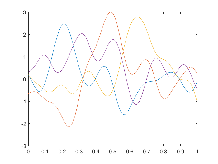
We demonstrate and on the following Gaussian processes , , on , where , with
| (78) |
In the experiments, we fix . Figure 1 shows samples of these processes for .
(i) Let be randomly chosen from , where . We plot in Figures 1 and 2 the following divergences between and : (squared Hilbert-Schmidt), (squared Wasserstein), and (Sinkhorn, and ).
(ii) Consider two sets of sample paths from each process, each path sampled at points , which are randomly chosen and fixed in advance from . We then compute the different divergences using Algorithm 1, for (Figure 3).
In agreement with theory, the convergence of the Sinkhorn divergence and Hilbert-Schmidt distance, being dimension-independent, is consistent across different dimensions, whereas the convergence of the Wasserstein distance is slower the larger the dimension is.


.


10 Proofs of main results
Proof of Lemma 5.
It suffices to prove this for the case . Let be any orthonormal basis in , then
Proof of Lemma 6.
For any , ,
showing that . It follows that for any ,
It follows that, in the , the matrix representation of is .
Lemma 25 (Corollary 5 in [35]).
For ,
| (79) |
Corollary 26.
For ,
| (80) |
Lemma 27 (Corollary 6 in [35]).
For ,
| (81) |
Proof of Proposition 8.
Proof of Proposition 10.
Proof of Theorem 11.
Proof of Propositions 12.
Define the random variables by , , where is independently sampled from . The ’s are IID, with and . By Lemma 36,
Define the random variable by . Since the ’s are IID,
By Chebyshev inequality, for any , . Let , then . Similarly, since , we have . Computing the intersection of these two sets of events and replacing by , we obtain the desired bounds.
Proof of Theorem 13.
Proof of Lemma 24.
Since , we have , thus -almost surely. By Hölder Theorem and Tonelli Theorem,
If , then for each fixed , we have . Thus
by using the integral (see Formula 7.4.4 in [1]).
Proof of Proposition 14.
We have by Proposition 10. Define the map by . Let , , be IID -valued random variables defined by , where is independently sampled from . Then
by Lemma 24. Define by . Since the ’s are independent, identically distributed,
By Chebyshev inequality, for any , . Let , then . Similarly, . Computing the intersection of these two events and replacing by , we obtain the desired bounds.
Proof of Theorem 15.
With each pair , by Theorem 2,
For , by Proposition 14, the following sets satisfy , ,
Let , then and ,
Proof of Theorem 16.
Lemma 28.
Under Assumptions , let be independently sampled from . For any , with probability at least ,
| (82) |
Proof.
Define the random variable by , then and , . The desired bound then follows from Proposition 9.
Lemma 29 (Lemma 4.1 in [41]).
For ,
| (83) |
Proof of Theorem 17.
The following is a special case of Corollary 4 in [35], where and are the sample mean and sample covariance matrix, respectively, based on the sample .
Proposition 30 (Estimation of 2-Wasserstein distance between Gaussian measures on ).
Let on , . Let and be independently sampled from and , respectively. , with probability at least ,
| (84) |
where , .
Proof of Theorem 19.
Lemma 31.
Under Assumptions 1-4, ,
| (85) |
Proof.
By Hölder Theorem and Tonelli Theorem, , ,
Thus . By Fubini Theorem,
Proof of Proposition 21.
Define random variable by , where is independently sampled from . Then the ’s are IID and , , and
Define the random variable by . Since the ’s are independent, identically distributed,
By the Chebyshev inequality, for any , . Let , then . Similarly, since , we have . Computing the intersection of these two sets, replacing with , gives us the desired result.
Proof of Theorem 22.
11 Estimation of Hilbert-Schmidt distance
For completeness, we present the finite sample estimate of . For this, it is not necessary to assume that , are self-adjoint, positive. The only requirement is that .
Assumption 7. Let be a complete, separable metric space, a Borel probability measure on . Let be pointwise defined. Assume such that
| (86) |
It is well-known (see e.g. Theorem VI.23 in [44]) that the following operator (similarly , ) is Hilbert-Schmidt
| (87) |
Theorem 32 (Estimation of Hilbert-Schmidt distance).
Under Assumption 7, let , be independently sampled from . Let be defined by , , . , with probability at least ,
| (88) |
Lemma 33.
Under Assumption 7, let , be independently sampled from . , with probability at least ,
| (89) |
Proof.
12 Hilbert-Schmidt operators between two Hilbert spaces
For completeness, we include here several properties of the set of Hilbert-Schmidt operators between two separable Hilbert spaces and . Many standard texts in functional analysis consider the set , with . The definition of that we use here is from [23]
| (90) |
where the Hilbert-Schmidt norm is defined by
| (91) |
for any orthonormal bases of , , independently of the choice of bases.
Proposition 34.
Let be two separable Hilbert spaces. Let . Then and .
Proof.
Consider the polar decomposition where is a partial isometry on , i.e. an isometry on the closed subspace . Let be an orthonormal basis in , then is also an orthonormal basis in and
where the last inequality is an equality if , i.e. .
Corollary 35.
Let be two separable Hilbert spaces. Let . Then and
| (92) |
Lemma 36.
Let be two separable Hilbert spaces. Let . Then and .
Proof.
Let be any orthonormal basis in . By definition, .
References
- [1] M. Abramowitz and I. Stegun, Handbook of Mathematical Functions With Formulas, Graphs, and Mathematical Tables, Applied Mathematics Series 55, National Bureau of Standards, 1972.
- [2] V. Bogachev, Gaussian Measures, American Mathematical Society, 1998.
- [3] J. Borwein, A. Lewis, and R. Nussbaum, Entropy minimization, DAD problems, and doubly stochastic kernels, Journal of Functional Analysis, 123 (1994), pp. 264–307.
- [4] I. Csiszár, I-divergence geometry of probability distributions and minimization problems, The Annals of Probability, (1975), pp. 146–158.
- [5] F. Cucker and S. Smale, On the mathematical foundations of learning, Bulletin of the American Mathematical Society, 39 (2002), pp. 1–49.
- [6] J. Cuesta-Albertos, C. Matrán-Bea, and A. Tuero-Diaz, On lower bounds for the L2-Wasserstein metric in a Hilbert space, Journal of Theoretical Probability, 9 (1996), pp. 263–283.
- [7] M. Cuturi, Sinkhorn distances: Lightspeed computation of optimal transport, in Advances in neural information processing systems, 2013, pp. 2292–2300.
- [8] M. Cuturi and G. Peyré, Computational optimal transport, Foundations and Trends® in Machine Learning, 11 (2019), pp. 355–607.
- [9] E. del Barrio and J.-M. Loubes, The statistical effect of entropic regularization in optimal transportation, preprint arxiv:2006.05199, (2020).
- [10] D. C. Dowson and B. V. Landau, The Fréchet distance between multivariate normal distributions, Journal of multivariate analysis, 12 (1982), pp. 450–455.
- [11] R. Dudley, The speed of mean glivenko-cantelli convergence, The Annals of Mathematical Statistics, 40 (1969), pp. 40–50.
- [12] F. Ferraty and P. Vieu, Nonparametric functional data analysis: theory and practice, Springer, 2006.
- [13] J. Feydy, T. Séjourné, F.-X. Vialard, S. Amari, A. Trouve, and G. Peyré, Interpolating between optimal transport and MMD using Sinkhorn divergences, in International Conference on Artificial Intelligence and Statistics, 2019.
- [14] N. Fournier and A. Guillin, On the rate of convergence in wasserstein distance of the empirical measure, Probability Theory and Related Fields, 162 (2015), pp. 707–738.
- [15] S. Fremdt, J. Steinebach, L. Horváth, and P. Kokoszka, Testing the equality of covariance operators in functional samples, Scandinavian Journal of Statistics, 40 (2013), pp. 138–152.
- [16] M. Gelbrich, On a formula for the L2 Wasserstein metric between measures on Euclidean and Hilbert spaces, Mathematische Nachrichten, 147 (1990), pp. 185–203.
- [17] A. Genevay, L. Chizat, F. Bach, M. Cuturi, and G. Peyré, Sample Complexity of Sinkhorn Divergences, in International Conference on Artificial Intelligence and Statistics, 2019, pp. 1574–1583.
- [18] A. Genevay, G. Peyre, and M. Cuturi, Learning Generative Models with Sinkhorn Divergences, in Proceedings of the International Conference on Artificial Intelligence and Statistics, 2018.
- [19] C. Givens and R. Shortt, A class of Wasserstein metrics for probability distributions., The Michigan Mathematical Journal, 31 (1984), pp. 231–240.
- [20] J. Horowitz and R. Karandikar, Mean rates of convergence of empirical measures in the wasserstein metric, Journal of Computational and Applied Mathematics, 55 (1994), pp. 261–273.
- [21] L. Horváth and P. Kokoszka, Inference for Functional Data with Applications, Springer, 2012.
- [22] H. Janati, B. Muzellec, G. Peyré, and M. Cuturi, Entropic optimal transport between (unbalanced) Gaussian measures has a closed form, Advances in Neural Information Processing Systems, (2020).
- [23] R. Kadison and J. Ringrose, Fundamentals of the theory of operator algebras. Volume I: Elementary Theory, Academic Press, 1983.
- [24] M. Knott and C. Smith, On the optimal mapping of distributions, Journal of Optimization Theory and Applications, 43 (1984), pp. 39–49.
- [25] C. Léonard, A survey of the Schrödinger problem and some of its connections with optimal transport, Discrete & Continuous Dynamical Systems-A, 34 (2014), pp. 1533–1574.
- [26] A. Mallasto, Estimating 2-Sinkhorn divergence between Gaussian processes from finite-dimensional marginals, arXiv preprint arXiv:2102.03267, (2021).
- [27] A. Mallasto and A. Feragen, Learning from uncertain curves: The 2-wasserstein metric for Gaussian processes, in Advances in Neural Information Processing Systems, 2017, pp. 5660–5670.
- [28] A. Mallasto, A. Gerolin, and H. Minh, Entropy-regularized 2-Wasserstein distance between Gaussian measures, preprint arXiv:2006.03416, (2020).
- [29] V. Masarotto, V. Panaretos, and Y. Zemel, Procrustes metrics on covariance operators and optimal transportation of gaussian processes, Sankhya A, 81 (2019), pp. 172–213.
- [30] A. Matthews, J. Hensman, R. Turner, and Z. Ghahramani, On sparse variational methods and the Kullback-Leibler divergence between stochastic processes, in Artificial Intelligence and Statistics, PMLR, 2016, pp. 231–239.
- [31] G. Mena and J. Niles-Weed, Statistical bounds for entropic optimal transport: sample complexity and the central limit theorem, in Advances in Neural Information Processing Systems, 2019, pp. 4541–4551.
- [32] H. Minh, Some properties of Gaussian reproducing kernel Hilbert spaces and their implications for function approximation and learning theory, Constructive Approximation, 32 (2010), pp. 307–338.
- [33] H. Minh, Entropic regularization of Wasserstein distance between infinite-dimensional Gaussian measures and Gaussian processes, preprint arXiv:2011.07489, (2020).
- [34] H. Minh, Regularized divergences between covariance operators and Gaussian measures on Hilbert spaces, Journal of Theoretical Probability, (2020).
- [35] H. Minh, Convergence and finite sample approximations of entropic regularized Wasserstein distances in Gaussian and RKHS settings, arXiv preprint arXiv:2101.01429, (2021).
- [36] I. Olkin and F. Pukelsheim, The distance between two random vectors with given dispersion matrices, Linear Algebra and its Applications, 48 (1982), pp. 257–263.
- [37] V. Panaretos, D. Kraus, and J. Maddocks, Second-order comparison of Gaussian random functions and the geometry of DNA minicircles, Journal of the American Statistical Association, 105 (2010), pp. 670–682.
- [38] G. Patrini, R. Berg, P. Forre, M. Carioni, S. Bhargav, M. Welling, T. Genewein, and F. Nielsen, Sinkhorn Autoencoders, Uncertainty in Artificial Intelligence, (2020).
- [39] D. Pigoli, J. Aston, I. Dryden, and P. Secchi, Distances and inference for covariance operators, Biometrika, 101 (2014), pp. 409–422.
- [40] I. Pinelis, Optimum bounds for the distributions of martingales in Banach spaces, The Annals of Probability, (1994), pp. 1679–1706.
- [41] R. Powers and E. Størmer, Free states of the canonical anticommutation relations, Communications in Mathematical Physics, 16 (1970), pp. 1–33.
- [42] B. Rajput and S. Cambanis, Gaussian processes and Gaussian measures, The Annals of Mathematical Statistics, (1972), pp. 1944–1952.
- [43] J. Ramsay and B. Silverman, Functional data analysis, Springer, 2005.
- [44] M. Reed and B. Simon, Methods of Modern Mathematical Physics: Functional analysis, Academic Press, 1975.
- [45] L. Rosasco, M. Belkin, and E. D. Vito, On learning with integral operators, Journal of Machine Learning Research, 11 (2010), pp. 905–934.
- [46] L. Rüschendorf and W. Thomsen, Closedness of sum spaces and the generalized schrödinger problem, Theory of Probability & Its Applications, 42 (1998), pp. 483–494.
- [47] E. Schrödinger, Über die umkehrung der naturgesetze, Verlag Akademie der wissenschaften in kommission bei Walter de Gruyter u. Company, 1931.
- [48] S. Smale and D. Zhou, Learning theory estimates via integral operators and their approximations, Constructive Approximation, 26 (2007), pp. 153–172.
- [49] H. Sun, Mercer theorem for RKHS on noncompact sets, Journal of Complexity, 21 (2005), pp. 337–349.
- [50] S. Sun, G. Zhang, J. Shi, and R. Grosse, Functional variational Bayesian neural networks, International Conference on Learning Representation, (2019).
- [51] C. Villani, Topics in Optimal Transportation, vol. 58 of Graduate Studies in Mathematics, American Mathematical Society, 2016.
- [52] J. Weed and F. Bach, Sharp asymptotic and finite-sample rates of convergence of empirical measures in Wasserstein distance, Bernoulli, 25 (2019), pp. 2620–2648.