∎
Methods of Continuation and their Implementation in the COCO Software Platform with Application to Delay Differential EquationsJournal: Nonlinear Dynamics
Abstract
This paper treats comprehensively the construction of problems from nonlinear dynamics and constrained optimization amenable to parameter continuation techniques and with particular emphasis on multi-segment boundary-value problems with delay. The discussion is grounded in the context of the coco software package and its explicit support for community-driven development. To this end, the paper first formalizes the coco construction paradigm for augmented continuation problems compatible with simultaneous analysis of implicitly defined manifolds of solutions to nonlinear equations and the corresponding adjoint variables associated with optimization of scalar objective functions along such manifolds. The paper uses applications to data assimilation from finite time histories and phase response analysis of periodic orbits to identify a universal paradigm of construction that permits abstraction and generalization. It then details the theoretical framework for a coco-compatible toolbox able to support the analysis of a large family of delay-coupled multi-segment boundary-value problems, including periodic orbits, quasiperiodic orbits, connecting orbits, initial-value problems, and optimal control problems, as illustrated in a suite of numerical examples. The paper aims to present a pedagogical treatment that is accessible to the novice and inspiring to the expert by appealing to the many senses of the applied nonlinear dynamicist. Sprinkled among a systematic discussion of problem construction, graph representations of delay-coupled problems, and vectorized formulas for problem discretization, the paper includes an original derivation using Lagrangian sensitivity analysis of phase-response functionals for periodic-orbit problems in abstract Banach spaces, as well as a demonstration of the regularizing benefits of multi-dimensional manifold continuation for near-singular problems analyzed using real-time experimental data.
†† Note: This preprint has not undergone peer review (when applicable) or any post-submission improvements or corrections. The Version of Record of this article is published in Nonlinear Dynamics, and is available online at https://doi.org/10.1007/s11071-021-06841-1Keywords:
delay differential equations multi-segment boundary-value problems implicitly defined manifolds problem regularization constrained optimization Lagrange multipliers adjoint equations graph representations phase response curves1 Introduction
We use this section to describe the objectives of this paper and to place its content in the context of the ongoing development of software tools for continuation-based analysis of nonlinear dynamical systems. An overview of the original contributions along with section-wise descriptions of the content is also provided.
1.1 Motivation
While the possibility of closed-form analysis is fortuitous and perhaps career-changing, computation is the bread and butter of applied research in nonlinear dynamics. Computational techniques derive their power from rigorous mathematical analysis, but extend far beyond the reach of theoretical tools (see, e.g., the analysis of global bifurcations of the Lorenz manifold in doedel2006global; guckenheimer2015invariant). With their aid, systematic exploration becomes possible, e.g., of the dependence of system responses on model parameters abbas2011parametric, the sensitivity of these responses to parameter uncertainty kewlani2012polynomial, and the determination of optimal selections of parameter values amandio2014stochastic; koh2016optimizing. Such exploration inspires further theoretical advances, including of methods for projecting the dynamics of large-scale systems onto reduced-order models haller2016nonlinear; szalai2019model; szalai2020invariant; touze2006nonlinear, amenable to efficient computation and powerful visualization.
Continuation methods are a class of deterministic computational techniques for exploring smooth manifolds of solutions to nonlinear equations dankowicz2013recipes; krauskopf2007numerical. By now classical algorithms convert common questions of interest to applied dynamicists into such nonlinear equations, enabling their analysis using continuation. Prominent among such uses are bifurcation analyses of equilibria govaerts2000numerical, periodic orbits munoz2003continuation, connecting orbits beyn1990numerical, quasiperiodic invariant tori schilder2005continuation, and stable and unstable manifolds dellnitz1996computation for smooth and piecewise-smooth vector fields, including in problems with delay barton2009stability; chavez2020numerical; luzyanina1997computation; roose2007continuation. By their versatility, continuation methods are an invaluable tool in the researcher’s arsenal.
It is the aim of this review to invite new generations of dynamicists to the world of continuation methods while also giving the seasoned researcher plenty of original fodder for thought. The paper purposely avoids stepping over well-trodden ground dealing with the specific algorithms used to cover solution manifolds or with examples of bifurcation analysis, as these topics have been discussed in great detail in a number of key sources allgower2003introduction; kuznetsov2013elements. Instead, completely new content develops a formalism for problem construction, inspired by functionality available in the coco software platform COCO, illustrates its use on problems from data assimilation and phase response analysis, and applies its principles to the detailed construction of a toolbox for analyzing a large class of (possibly non-autonomous) multi-segment boundary-value problems with delay.
Given the ambitious scope and the anticipated range of reader expertise, the paper is intentionally self-contained and designed to address both deductive and inductive learning styles. Emphasis is placed on a formalism that translates directly to computational encoding, say, in the coco framework. Examples are drawn from the existing literature but retrofitted to the universal abstractions proposed in this manuscript. Where appropriate, the text highlights opportunities for practice or more substantial further development. For that is ultimately the measure of this paper’s value; the extent to which it spurs original creativity and innovation.
1.2 Software design
There is a natural tension in both theoretical and computational research between the particular and the general. One of us (HD) spent half of his professional career implementing continuation methods on a just-in-time basis. With each new problem, old code scripts were dusted off, debugged, and redeployed. The investment to do anything beyond solving particular problems seemed overwhelming and perhaps not professionally rewarding. But the general beckoned. And others had long before chosen that road, aiming to build translational tools that would bring nonlinear dynamics to the scientific masses back1992dstool; kuznetsov1997content. In so doing, a balance again had to be struck between the particular and the general, between utility and universality. To this day, several of the outcomes of this effort continue to provide invaluable access to the insights of the qualitative theory of dynamical system also to non-experts. These include auto doedel2007auto and the wrapper xppaut ermentrout2002simulating, a popular choice for continuation-based analysis of ordinary differential equations (ODEs), matcont dhooge2003matcont for ODEs/maps, dde-biftool engelborghs2002numerical; ddebiftoolmanual and knut Kunt for delay differential equations (DDEs), pde2path kuehn2015efficient; uecker2014pde2path for partial differential equations (PDEs), and hompack watson1987algorithm for globally-convergent homotopy analysis of arbitrary nonlinear equations.
With an emphasis on utility, these packages were designed to address specific problem classes/types, while leaving open the possibility of additional creative uses (e.g., the development of special purpose wrappers for auto for computing invariant manifolds manbvp england2005computing, bifurcation analysis of Filippov systems slidecont dercole2005slidecont, bifurcation analysis of periodic orbits in hybrid dynamical systems thota2008tc, and the computation of global isochrons in osinga2010continuation). In contrast, an emphasis on universality was the guiding principle behind the creation of the coco software package. Instead of building solutions, build a tool that others could use to build solutions. Define the platform, the language of discourse, and the paradigm of problem construction and analysis. Make it easy to pursue the particular and yet worthwhile to support the general. Reward a tight coupling between rigorous mathematics and computational encoding. Invite the community to innovate and substitute, benefiting from a prescribed interface.
An important step in this direction was the decoupling of problem construction from problem analysis. After all, the nonlinear equations analyzed using continuation methods could also be the target of iterative and even stochastic techniques that made no use of the manifold nature of their solutions boender1982stochastic; byrd2000trust. And while other packages emphasized analysis of one-dimensional solution manifolds (with some exceptions, e.g., manpak rheinboldt1996manpak and multifario henderson2002multiple), there was really no good reason to impose this restriction at the stage of problem construction. The real breakthrough, however, was in conceiving of a modular and staged construction paradigm, respecting an oft-occurring arrangement of the problem unknowns into densely coupled communities with sparse coupling to other communities (per the terminology of network science porter2009communities). A powerful application was found in multi-segment boundary-value problems (BVPs), e.g., periodic orbits in hybrid dynamical systems, in which boundary conditions between segments represent such sparse coupling between groups of unknowns separately parameterizing individual segments dankowicz2011extended.
As implemented in coco, this construction paradigm leveraged an object-oriented perspective, conceiving of a system of equations as decomposed into multiple object instances, describing subsets of equations and unknowns with inherent meaning, coupled together through appropriate gluing conditions (cf. the terminology used in multibody systems otter1996modeling; schiehlen2013advanced). With the recognition of common examples of mathematical objects (e.g., equilibria, trajectory segments, and periodic orbits) as constituting abstract classes of equations and unknowns, there resulted a hierarchy of problem construction whereby new abstract classes could be constructed from the composition of existing ones, and different versions of existing abstract classes could be substituted at will. As an example, problems involving the simultaneous analysis of an equilibrium (E), a periodic orbit (P), and an E-to-P connecting orbit were constructed with ease by leveraging existing abstract classes for each of these objects, glued together with a sparse set of boundary conditions dankowicz2013recipes; dankowicz2011continuation; krauskopf2008lin.
With the recognition of problem construction as distinct from problem analysis, more emphasis could also be placed on developing alternative approaches to continuation along solution manifolds, including the possibility of analysis along multi-dimensional manifolds. Where such algorithms in other packages were more tightly connected to the particular defining problems, the implementation in coco sought to remain agnostic as to the origin of the system of governing equations. This level of generality, of course, came at a cost as the particular solutions specific to a problem class could not be anticipated a priori. A satisfactory solution to this tension, also generalizable to the multi-dimensional case, was arrived at only in the past few years dankowicz2020multidimensional; yuqing2018thesis.
With these observations in mind, it is clear that software design has become a matter worthy of independent study, also to the community of nonlinear dynamics researchers. Moreover, with the appropriate attention to its theoretical underpinnings, such study also comes with scholarly reward. One example is the recent expansion to the original staged construction paradigm of coco in support of the parallel staged construction of (a critical subset of) the adjoint necessary conditions for extrema along constraint manifolds li2017staged; li2020optimization. This expansion reflects the decomposition of a problem Lagrangian into a sum of individual constraints linearly paired with corresponding adjoint variables (also called dual variables or Lagrange multipliers) that measure the sensitivities of an objective function to constraint violations at stationary points of the Lagrangian. Since the Lagrangian is linear in the adjoint variables, the contributions to the adjoint conditions from each term of the Lagrangian are also linear in the adjoint variables ahsan2020optimization. The complete set of adjoint conditions may therefore again be built in stages in a one-to-one mapping to the stages used to construct the full set of constraints.
It is one aim of this review to describe in detail this staged construction paradigm in a manner compatible with the implementation in coco but sufficiently abstract to allow for independent implementation. The effort involved in such independent development may be appreciated by reference to the history of coco.
1.3 A brief history of coco
The software package coco is the result of joint development since 2007 by Harry Dankowicz and Frank Schilder, and, since 2016, Mingwu Li mingwu2020thesis, with additional contributions from Michael E. Henderson, Erika Fotsch fotsch2016thesis, and Yuqing Wang yuqing2018thesis. Helpful feedback and contributions are also acknowledged from Jan Sieber and David Barton, and a growing user community barton2017control; cao2019nonlinear; heitmann2021arrhythmogenic; liu2017controlling; ponsioen2018automated; zhong2020global. Extensive discourse on the original design philosophy and mathematical underpinnings of the coco platform is available in the textbook dankowicz2013recipes, which includes a large collection of template toolboxes and example problems.
The first official release of coco coincided with the publication of dankowicz2013recipes in 2013. This included code documentation and detailed demos from dankowicz2013recipes. The November 2015 release introduced fully documented, production-ready toolboxes for common forms of bifurcation analysis of equilibria and periodic orbits in dynamical systems. These provided support for continuation of
- •
equilibria in smooth dynamical systems using the ep toolbox;
- •
constrained trajectory segments with independent and adaptive discretizations in autonomous and non-autonomous dynamical systems using the coll toolbox; and
- •
single-segment periodic orbits in smooth, autonomous or non-autonomous dynamical systems, and multi-segment periodic orbits in hybrid, autonomous dynamical systems using the po toolbox.
The November 2017 release made significant updates to the coco core and library of toolboxes and demos to provide support for constrained design optimization on integro-differential boundary-value problems li2017staged. These updates enabled the staged construction of the adjoint equations associated with equality-constrained optimization problems, and provided support for adaptive remeshing of these equations in parallel with updates to the problem discretization of the corresponding boundary-value problems. The March 2020 release of coco extended this functionality to also allow for finite-dimensional inequality constraints, bounding the locus of extrema to an implicitly-defined feasible region li2020optimization.
The original release of coco included the default atlas algorithm atlas_1d for one-dimensional solution manifolds. This was accompanied by a discussion in Parts III and IV of dankowicz2013recipes that described a general methodology for building atlas algorithms and also included an example of a two-dimensional atlas algorithm with fixed step size for non-adaptive continuation problems, inspired by Henderson’s multifario package henderson2002multiple. A fully step-size-adaptive implementation of multifario as a coco-compatible atlas algorithm for multi-dimensional manifolds of solutions to non-adaptive continuation problems was included as an alpha version in the November 2017 release. The March 2020 release of coco included the updated atlas algorithm atlas\_kd for multi-dimensional solution manifolds for adaptive continuation problems with varying embedding dimension and interpretation of problem unknowns dankowicz2020multidimensional. Usage of the atlas_1d and atlas\_kd atlas algorithms, as well as the basic coco constructors and utilities and those particular to the ep, coll, and po toolboxes is illustrated in numerous examples in tutorial documents included with the coco release. Each example corresponds to fully documented code in the release.
One of the purported strengths of the coco package vis-à-vis its peers is its extensibility blyth2020. For example, it has not been the intent of the coco development to build graphical user interfaces to the methods and data invoked and processed during analysis of a continuation problem, although some low-level data processing and visualization routines are included with the coco core. Instead, support for run-time access to data is available in coco, for example, through a signal-and-slot mechanism as described in dankowicz2013recipes. Such a communication protocol allows independent development of user interfaces without modifications to the core. An example of such independent development is the analysis of hybrid dynamical systems described in chong2016numerical using a graphical user interface to the coco core and the po toolbox. New classes of problems may also be analyzed using coco without a preexisting toolbox for this purpose. Examples include the coupling in formica2013coupling of coco and the po toolbox with the comsol multiphysics finite element software, the analysis of quasiperiodic invariant tori in li2020tor using the coll toolbox, and the integration of the construction of spectral submanifolds in ssmtool2 with frequency response analysis using the ep and po toolboxes. With the help of suitable wrappers, the data structures generated by the coco construction methodology may also be used by non-coco computational algorithms. An example is the application in coco-fmincon of the matlab function foptim to the continuation problem constructed using coco.
Sophisticated users may also wish to build new toolboxes for others to use. Advanced techniques for bifurcation detection, normal-form analysis, and so on, can be implemented using well-defined interface functions. An example is the implementation in coco-shoot of shooting techniques for continuation of periodic orbits using coco. Another example is the toolbox ddebiftool\_coco that provides coco-compatible access to the defining systems and monitoring functions created by dde-biftool for bifurcation analysis of DDEs ddebiftoolmanual, thereby benefiting from the atlas algorithms and nonlinear solvers of coco. A further example is the work by Schilder et al. schilder2015experimental to develop a coco-compatible toolbox for noise-contaminated zero problems as occur when performing continuation in experiments barton2012control; renson2016robust; renson2019application; renson2019numerical. Shipped with the coco release, their continex toolbox includes an original atlas algorithm and nonlinear solver designed to track one-dimensional solution manifolds given low-precision numerics and high costs for evaluating residuals and their sensitivities.
1.4 Contributions of this paper
Rather than a mere review of the state-of-the-art in continuation methods and their applications, this paper makes several original contributions that are not covered elsewhere. These contributions are conceptual and structural and point to innovations in software design of the sort discussed above. They expand access to known solutions, rather than offer new solutions to known problems.
Foremost among these contributions is a detailed guide for the construction of a coco-compatible toolbox for analyzing families of solutions to multi-segment boundary-value problems with discrete delays, as well as for finding stationary points of scalar-value objective functions along such families (see bartoszewski2011solving; calver2017numerical; chai2013unified; engelborghs2001collocation; gollmann2009optimal; khasawneh2011multi; shinohara2007boundary; TraversoMagri2019, especially gollmann2009optimal; TraversoMagri2019 for a similar usage of auxiliary variables to represent time-delayed terms). Not only does such a toolbox not exist previously for coco, but is also not available through other packages. The ddebiftool\_coco toolbox mentioned above, for example, is not designed to couple multiple trajectory segments and lacks tools for automatic construction of the adjoint contributions. By adhering to the object-oriented construction paradigm, the treatment in this paper demonstrates how very general classes of boundary-value problems may be addressed within a single framework, avoiding the need to develop individual solutions for periodic orbits, quasiperiodic orbits, connecting orbits, initial-value problems, and optimal control problems.
Prominent among the additional contributions of this paper is a detailed discussion of a data assimilation problem with delay inspired by the analysis in TraversoMagri2019. Here, a constraint Lagrangian is used to generate explicit adjoint conditions in a form amenable to a continuation-based analysis per the successive continuation framework in ahsan2020optimization; li2017staged; li2020optimization as an alternative to the gradient-based optimization approach of TraversoMagri2019. In contrast to TraversoMagri2019, the discussion highlights the natural decomposition of the governing constraints into a multi-segment boundary-value problem, the linear dependence on suitably defined adjoint variables, and the way in which time delay in the governing differential constraints translates into time-advanced terms in the adjoint differential equations.
A contribution of unexpected importance is the original derivation using a Lagrangian formalism of the governing equations for computing phase response curves associated with limit cycles in a general Banach-space setting (in contrast, e.g., to izhikevich1997weakly where derivation is based on the adjoint equation of the reduced phase models). This treatment demonstrates how a phase response functional may be constructed from the adjoint variables associated with the sensitivities of the orbital period to violations of the differential constraints and periodic boundary conditions. As the adjoint conditions may again be constructed automatically from variations of a constraint Lagrangian, the discussion points to the immediate use of coco-compatible toolboxes that provide such support without the need for further development. This is in contrast to support for phase response analysis in other software packages, for example matcont dhooge2003matcont, which implement a reduced set of adjoint differential equations, boundary conditions, and normalization conditions that must be derived separately for each class of problem. Importantly, the Lagrangian foundation developed in this paper also suggests that out-of-the-box use of existing coco toolboxes for limit cycles in hybrid dynamical systems (e.g., piecewise-smooth vector fields) would permit such phase response analysis.
Finally, of notable mention is an original discussion of the benefits of multi-dimensional continuation for managing uncertainty in singularly-perturbed or noise-contaminated problems, for example applications involving experimental data. In such cases, uncertain input data or randomly disturbed residuals (caused by measurement errors) may result in a dramatic degree of output uncertainty even if single-parameter continuation were computationally feasible. As shown in this paper, however, this singular behavior may be regulated or entirely eliminated using multi-dimensional continuation independently of the value of the damping.
1.5 Organization of this paper
The body of this paper is divided into four sections book-ended by the present introduction and a concluding discussion in Section 6. Section 2 develops the principles of staged problem construction for the so-called augmented continuation problem, amenable to analysis of constraint manifolds and optimization along such manifolds. Several examples are used to first motivate this framework and, subsequently, illustrate its application to advanced analysis of problems with delay. A pattern of universality uncovered by the treatment in Section 2 is converted into a rigorous mathematical formalism for a coco-compatible toolbox for multi-segment boundary-value problems with discrete delays in Section 3. Straightforward generalizations of the toolbox and applications to the computation of phase response curves for limit cycles, homoclinic connections, quasiperiodic invariant tori, and optimal control inputs are considered in Section 4. The text then turns briefly to opportunities for further development of the basic toolbox functionality in Section 5.
Several parts of the discussion in Section 2 may be read independently from the remainder of the text, although clearly at some loss to the continuity of the flow. This certainly applies to the description of the coco formalism in Section 2.4 and to the applications to data assimilation in Section 2.5 (except for Section 2.5.3 and parts of Section 2.5.4) and phase response analysis in Section 2.6 (except for Section 2.6.4). The discussion of problem discretization in Section 3.4 may be skipped on a first reading. For the reader interested in the detailed implementation or considering an independent development, this section stresses the importance of systematic notation and rigor also in the encoding of a problem in order to ensure code verifiability. Finally, while the ordering of the text implies a natural flow, at times a nonlinear approach to reading this review may be appropriate. The reader may wish to skip ahead to anticipate the implications of the design decisions or return to an earlier section to better appreciate its purpose. That is encouraged.
2 Problem formulation
It is customary in treatments of continuation methods (e.g., doedel2007lecture) to begin with a discussion of the implicit function theorem, as the theoretical foundation for analyzing solutions of abstract nonlinear problems. Such a discussion naturally concerns itself with a decomposition of the unknowns into independent and dependent variables, and establishes conditions under which such a decomposition makes (local) sense. These conditions are then leveraged to give meaning to the notion of continuation: the local and continuous expansion of the known universe of solutions along implicitly defined manifolds.
Here, we largely depart from such a focus on solutions and their geometry by instead emphasizing the process of problem construction. Our concern is not principally with the techniques used to perform continuation, but with a systematic approach to formulating problems amenable to continuation, without imposing any preferred decompositions among the problem unknowns. As we show in this section, such a problem-oriented focus may yield benefits also to the process of continuation, as different formulations are more or less well-conditioned. Nevertheless, our primary aim is to identify patterns and structure in the way common problems arise in the study of dynamical systems, and to build useful abstractions around such patterns.
It is instructive to begin this journey into methods of continuation and their implementations in software within the realm of problems amenable to closed-form analysis. Such analysis removes consideration of various numerical approximations, inevitable in a computational implementation, and offers an opportunity for code verification. For the particular examples considered in this section, it points to generalizations to nonlinear problems without closed-form solutions. More importantly, it illustrates principles of intuitive and flexible problem construction, partially agnostic to the final objectives of the analysis. We argue that such flexibility should take precedence in the engineering of general-purpose software for continuation problems.
2.1 Looking for inflection points
Many problems of interest in the analysis and control of nonlinear dynamical systems may be formulated as problems of constrained design optimization (see, e.g., the study of periodically forced bioreactors in d2010choice or bubble motion driven by acoustic forcing in toilliez2008optimized; wyczalkowski2003optimization). In this section, we consider the search for optimal points along manifolds of solutions to algebraic and/or differential constraints in terms of objective functions characterizing the local manifold geometry (for an applied context, see acharya2020non for a recent study of non-monotonic dependence of the response dynamics of premixed flames on forcing amplitude).
Specifically, along the family of steady-state periodic responses of a harmonically-excited, linear oscillator parameterized by the excitation frequency , at most two values of correspond to local extrema in the rate of change of the response amplitude with respect to , as shown in the left panel of Fig. 1. To locate these values, we write the governing equation in the normalized form
| (1) |
make the ansatz for , and obtain
| (2) |
Differentiation twice with respect to then yields inflection points at the roots of the polynomial
| (3) |
or, equivalently, at points with
| (4) |
as illustrated in the right panel of Fig. 1. It follows that only one such root exists for , whereas two roots bracket the global maximum of the response amplitude at for . At these points, the response amplitude is given by
| (5) |
and , respectively, as shown in Fig. 2.


In lieu of the analysis afforded by the explicit expression (2) for the response amplitude, consider the equations
| (6) |
obtained by substitution of the ansatz in (1). To locate inflection points in the response amplitude , we may directly constrain a finite-difference approximation of its second derivative per the collection of polynomial constraints
| (7) | |||
| (8) | |||
| (9) | |||
| (10) | |||
| (11) |
in the limit as . As an alternative, consider instead the constrained optimization of the objective function with respect to in the limit as , given the polynomial constraints
| (12) | |||
| (13) | |||
| (14) |
By the calculus of variations gelfand2000calculus; liberzon2011calculus, we obtain necessary conditions for such loci of optimality by considering vanishing variations of a suitably constructed constraint Lagrangian. Here, such an analysis results in the constraints (12)-(14) coupled with the adjoint conditions
| (15) | |||
| (16) | |||
| (17) | |||
| (18) | |||
| (19) |
in terms of the Lagrange multipliers through that describe the sensitivity of the objective function at stationary points to violations of each of the constraints (12)-(14). Solutions are obtained only for and that satisfy the equation
| (20) |
or, equivalently,
| (21) |
again yielding the condition (3) on from the previous paragraph. In this case, imply that
| (22) | |||
| (23) | |||
| (24) |
The reader is encouraged to verify the claim regarding the relationship between these values of the Lagrange multipliers and the sensitivity of the objective function at stationary points to constraint violations. In contrast to the discussion that led directly to (3) in the first part of this section, we do not presuppose an explicit expression for the response amplitude, one that can be differentiated arbitrarily with respect to . Instead, we use a finite-difference approximation in terms of a fixed change in the independent variable and show that the predicted extremum converges to the desired solution when .
We may take a further step back from an explicit analysis by considering the constrained optimization with respect to of the objective function for , given the differential constraints
| (25) |
the boundary conditions
| (26) |
with and , and the algebraic constraint in the limit as . The boundary conditions ensure that solutions are periodic with local extrema at . In this case, the necessary conditions for optimality append to these constraints the adjoint conditions
| (27) | |||
| (28) | |||
| (29) | |||
| (30) | |||
| (31) | |||
| (32) | |||
| (33) |
in terms of the Lagrange multipliers through that describe the sensitivity of the objective function at stationary points to violations of the differential constraints (25), boundary conditions (26), or algebraic constraint , respectively. We again find that solutions exist only for and that satisfy (20), in which case, for example,
| (34) | |||
| (35) |
and
| (36) |
The reader is again encouraged to verify the claim regarding the relationship between these values of the Lagrange multipliers and the sensitivity of the objective function at stationary points to constraint violations. In contrast to the previous two approaches, we neither presuppose an explicit expression for the response amplitude nor for the form of the periodic response. Instead, the corresponding adjoint conditions (27)–(33) are here derived directly from the governing differential constraints and boundary conditions in a step that immediately generalizes to nonlinear problems for which closed-form solutions would not be available. As before, the finite-difference approximation in terms of a fixed change in the independent variable again approximates the loci of the inflection points to lowest order in .
For practice, it may be worthwhile to repeat this discussion in the simpler search for a local extremum in the response amplitude under variations in , known to exist at for . In this case, we might consider optimization of with respect to given the polynomial constraints
| (37) |
or optimization of with respect to given the boundary-value problem
| (38) |
Alternatively, we could consider imposition of the additional constraint to the polynomial constraints (12)-(14) in the limit as , or imposition of the additional constraint to the differential constraints (25), boundary conditions (26), and algebraic constraint in the limit as . In doing so, one should reasonably ask which of these approaches generalize to nonlinear boundary-value problems and to other objective functions.
2.2 Lessons and inspirations
The examples in the previous section are notably concerned not with a singular excitation response in isolation, but with a property of such a response in relation to nearby responses along a continuous (and locally differentiable) family of responses. Although we held fixed in our analysis, the implicit relationship in (3) further defines continuous families of inflection points and corresponding values of . We are inevitably drawn to a methodology for charting such continuous families and for monitoring the values of one or several objective functions along such families.
As we approach this task, a count of degrees of freedom proves useful. We generically reduce the number of degrees of freedom by one for every algebraic constraint imposed on an a priori unknown algebraic variable. Similarly, for every a priori unknown solution to a differential constraint, we generically append as many degrees of freedom as the number of required initial conditions. As an example, Eq. (3) imposes one algebraic constraint on two a priori unknown algebraic variables, yielding a problem with (generically) a single degree of freedom. Similarly, the seven constraints (12)-(14) constrain the ten a priori unknown algebraic variables , , , , , , , , , and to yield a problem with (generically) three degrees of freedom. The eight adjoint conditions (15)-(19) add seven more a priori unknown algebraic variables for a net of (generically) two degrees of freedom. Generically, the differential constraints (25), boundary conditions (26), and algebraic constraint on the a priori unknown variables , , , , , , , and result in a problem with three degrees of freedom. The adjoint conditions (27)-(33) add nine more a priori unknown variables for a net of (generically) two degrees of freedom.
The number of degrees of freedom of a differentiable continuation problem characterizes the dimension of a local manifold of solutions through any regular (in the sense of the implicit-function theorem krantz2012implicit) solution point. This dimension represents a deficit of constraints relative to the number of a priori unknown variables, and so we often speak of the dimensional deficit of a continuation problem. For all the continuation problems of interest here, the dimensional deficit is a finite number, even as the problem domain may be infinite dimensional.
Problems with zero dimensional deficit generically have at most isolated solutions doedel2007lecture. For example, by inspection of the partial derivative with respect to and , respectively, the roots of the multivariable polynomial in (3) are found to be locally unique with respect to for all positive (cf. the green square at the right panel of Fig. 1) and locally unique with respect to for all positive or (cf. the two magenta circles at the right panel of Fig. 1). By inspection of the Jacobian with respect to , , , , , , , , and through , solutions of the polynomial constraints (12)-(14) and the corresponding adjoint conditions (15)-(19) are locally unique with respect to and for all positive and sufficiently small . Similarly, by inspection of the Jacobian with respect to , , , , , , , , and through , solutions are found to be locally unique with respect to and for all positive or and sufficiently small . For solutions to the differential constraints (25), boundary conditions (26), algebraic constraint and the corresponding adjoint conditions (27)-(33), the same conclusions would be theoretically available by showing the invertibility of the linearization with respect to , , , , , , , , and through or , , , , , , , , and through , respectively. This undertaking is left to the reader.
Local uniqueness affords us confidence that an approximate algorithm to locate a solution to a problem with zero dimensional deficit will not be distracted by other nearby solutions. Provided that we initialize a search with an initial solution guess in the vicinity of the sought solution, we trust that a well-designed solver, e.g., based on Newton’s or Broyden’s methods kelley1995iterative, will rapidly converge to this solution. For the first two formulations of the inflection point problem in Section 2.1, we apply such a solver directly to the system of nonlinear equations. For the formulation in terms of differential boundary-value problems, some form of discretization must first be employed.
Inspired by these observations, a general continuation methodology for a problem with nonzero dimensional deficit may be obtained by iteratively
- •
constructing auxiliary constraints crisfield1983arc; dankowicz2013recipes; henderson2002multiple that when appended to result in a problem with zero dimensional deficit;
- •
constructing an initial solution guess for using a previously found solution to dankowicz2013recipes; govaerts2000numerical; seydel2009practical; and
- •
solving using an iterative algorithm based at the initial solution guess.
By definition, a solution to also solves . The success of such a methodology thus depends on its ability to ensure that solutions to are locally unique; that the iterative solver is able to converge to such a solution; and that the succession of such solutions suitably captures the geometry of the manifold of solutions to dankowicz2013recipes; guddat1990parametric.
Consider, for example, the problem obtained by replacing (15) in the necessary conditions for an extremum of under the polynomial constraints (12)-(14) with
| (39) |
For fixed and , we obtain a problem with nominal dimensional deficit equal to one, generically resulting in the existence of a unique one-dimensional solution curve through any regular solution point. In fact, by linearity and homogeneity of the adjoint conditions (15)-(19) with respect to and the Lagrange multipliers, one such curve is obtained from solutions to (12)-(14) together with . For the same reason, all solutions with nonzero lie on a straight line with and that satisfy (20) and Lagrange multipliers given by the right-hand sides of (22)-(24) multiplied by . Curiously, but not accidentally kernevez1987optimization; li2020optimization, the two curves intersect precisely at a local extremum of along the first curve, at a singular point of , as illustrated in the left panel of Fig. 3.

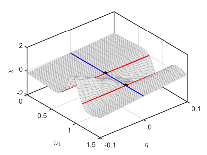
For this problem, at each iterate of the continuation methodology we construct by appending a single auxiliary constraint to . It comes as no surprise that trouble brews on a vicinity of the singular point as local uniqueness fails there for the sought solution to . With some luck, we may be able to step past the singularity along one of the curves, detect such a crossing, and then switch to the other curve. Such a branch-switching strategy kuznetsov2013elements; seydel2009practical may allow us to locate the sought inflection points starting from an arbitrary solution to (12)-(14) together with .
As an alternative, we seek to construct an augmented continuation problem by introducing one additional a priori unknown, say , such that the two solution curves to satisfy for . With a bit of care, all solutions of near the singular point of are regular points of . Here, we simply subtract from the left-hand side of (19) such that solutions to are obtained only for , , , and that satisfy the equation
| (40) |
For sufficiently small , it follows that the dimensional deficit of (two) equals the dimension of the solution manifold and all solutions near (and including) the singular point of are regular points of , as demonstrated in the right panel of Fig. 3. In this case, at each iterate of the continuation methodology we construct a problem with zero dimensional deficit by appending two auxiliary scalar constraints to .
As the reader may verify, an equivalent set of observations follows from
- •
the substitution of
(41) in lieu of (28) to generate a problem with nominal dimensional deficit equal to one, but with a singular point at the intersection of two one-dimensional curves of solutions ; followed by
- •
subtraction of from the left-hand side of (33) to obtain a problem with dimensional deficit equal to two and with all regular points on the corresponding solution manifold near (and including) the singular point of (obtained when ).
2.3 Regularizing nearly singular problems for low-precision numerics
Section 2.2 refers to general families of solutions, resulting from an arbitrary dimensional deficit, instead of just curves as is common in the literature. In the two examples, the construction of regularizes the continuation problem on a neighborhood of the singular point at the intersection of the solution curves to . The minimal dimension deficit required to remove the singularity is called the degree of degeneracy (or codimension) of the singularity kuznetsov2013elements. With a dimension deficit equal to two, we may continue through and past the singular point along a two-dimensional manifold of solutions to . As discussed in this section, continuation along multi-dimensional manifolds may also help address the increased demands on computational robustness in nearly singular problems in the presence of significant numerical uncertainty arnold1972lectures. This discussion is motivated by applications in which experimental data is used to evaluate the corresponding constraint residuals and their sensitivities with respect to the problem unknowns. When continuation is performed directly on physical experiments barton2012control; barton2017control; gonzalez2017assessing, these quantities are available only with low precision.
An example application is the analysis of the frequency response of weakly forced mechanical structures in the presence of small damping, e.g., the experimental data in Fig. 4 for a piezo-electric energy harvester obtained using control-based continuation in barton2012control. Here, small damping and dynamics conspire with low-precision numerics barton2017control to result in an apparent loss of smoothness of the recorded solution branch near the top of the resonance peak. For these operating conditions, we anticipate a resonance curve that is a small perturbation of the (zero-damping) singular limit represented by the backbone curve (obtained using continuation in experiments on purely mechanical structures in renson2016robust). For finite, but small, damping and fixed forcing phase and amplitude we expect problem condition numbers proportional to near the top of the resonance peak and for near its base.
To illustrate the regularizing benefits of multi-dimensional continuation in a case where they can be demonstrated explicitly, we consider again the linear harmonically forced oscillator. The equations
| (42) |
for fixed, small and under variations in are obtained from the ansatz substituted into the differential constraint
| (43) |
In contrast to Section 2.1, we here anticipate small values of the forcing amplitude preventing a reduction to the normal form in (1) using an scaling. We also keep the phase of the forcing free in (43).
As before, we may parameterize and explicitly in terms of , , and :
| (44) |
As a consequence, we obtain the rotational symmetry
| (45) |
In particular, for fixed , solutions lie on concentric circles in the plane of radii
| (46) |
and centered on the origin. These are when corresponding to a sharp resonance peak in the frequency-response diagram (see Fig. 5, bottom left panel).
We may explore the full 3-dimensional manifold of solutions to (42) by considering embedded submanifolds obtained, for example, by holding subsets of variables fixed. Consider, for example, the one-dimensional solution manifold obtained by holding both and fixed. We obtain the tangent space at each solution point from the nullspace of the Jacobian matrix of (42) with respect to , , and :
| (47) |
whose singular values equal
| (48) |
For , these are and , respectively. The smaller singular value of order will cause a great degree of uncertainty of the tangent direction if low-precision computations are performed in this asymptotic limit, even as the radius in (46) is . The right panel in Fig. 5 quantifies this sensitivity along the resonance peak in terms of the minimal singular value, parameterized using the phase of the response relative to the forcing (curve for fixed , ).
Consider, instead, the two-dimensional solution manifold obtained by holding the forcing amplitude fixed while allowing the phase of the forcing to vary. We may obtain the tangent space at each solution point from the nullspace of the Jacobian matrix of (42), augmented by a scaled equation keeping fixed, with respect to , , , , and :
| (49) |
By the rotational symmetry, without loss of generality, we may consider a point on the solution manifold with . At this point, the condition number of the matrix in (49) behaves as the inverse of the 2-norm of the columns of the top row of (49) which evaluates to
| (50) |
For this is . On the other hand, with the ansatz and , we find in the asymptotic limit that (50) has a local minimum of at , local maxima of at , and another pair of local minima of at . In Fig. 5, the curve for fixed shows the scaled inverse of (50). We thus see an improvement in the condition number across the resonance peak where the response amplitude is , except for the asymptotic limit , where low-precision computations again would result in a great degree of uncertainty of the corresponding tangent directions. To a lesser degree, increased uncertainty is exhibited also for the asymptotic limit .
As a third alternative, consider the two-dimensional manifold obtained by holding fixed at corresponding to fixing the phase of the forcing. Here, we obtain the tangent space at each solution point from the nullspace of the Jacobian matrix of (42), augmented by the equation , with respect to , , , , and :
| (51) |
The condition number of this matrix behaves as the inverse of the 2-norm of the columns of the second row of (51), which evaluates to
| (52) |
This is again for . On the other hand, the ansatz and yields local maxima and minima, respectively, in the asymptotic limit at
| (53) |
where the norm in (52) behaves as and , respectively. With this choice of fixed variables, we have entirely eliminated the poor performance with low-precision computations near the resonant peak, but retain increased uncertainty for the asymptotic limit . The right panel in Fig. 5 shows that the sensitivity curve for fixed is lower than the previous two approaches over most of the resonance peak, but still goes to infinity for .
We obtain the full three-dimensional solution manifold by allowing simultaneous variations in , , , , and . In this case, the tangent space at each solution point is obtained from the nullspace of the Jacobian matrix
| (54) |
whose condition number is everywhere as and may be obtained from the other three variables without the possibility of singularities. The right panel in Fig. 5 shows that the curve for sensitivity when continuing the full manifold is uniformly bounded for small .
While the above analysis was performed for the linear oscillator to permit explicit expressions for the computational sensitivity to low-precision numerics, its predictions remain qualitatively true also for nonlinear oscillators. This is illustrated in Fig. 5 for the forced Duffing oscillator (dotted curves obtained using the singular values of the Jacobian of a discretization of the nonlinear periodic-orbit problem) which exhibit similar asymptotic behavior in the limit as for the linear oscillator. The near constant ratio between the norm of the inverse of the Jacobian in the numerical implementation and the idealized analysis is (the number of collocation intervals used by the coll toolbox). We leave it to the reader to derive analytical predictions like those found in this section by applying an appropriate perturbation method to this nonlinear problem. We conclude that formulations with dimensional deficits greater than one should be considered whenever one-dimensional bifurcation diagrams appear sensitive to small changes in the problem.
2.4 The coco formalism
The discussion in Sections 2.2 and 2.3 highlights the merits of considering problem construction separately from problem analysis. First decide what you want to do. Then figure out how to do it. The description of the coco construction framework in this section continues in this spirit.
In the general case, we consider continuation problems of the form
| (55) |
for some Frechét differentiable operator with Banach space domain and range . At this level of abstraction, there are no distinguishing features of either domain or range. We do not unnecessarily presuppose a dimensional deficit nor assume a particular decomposition of . Instead, we design a general continuation methodology that is accommodating of different dimensional deficits and independent of any substructure of .
A specialized form of the continuation problem in (55) that self-referentially contains the form in (55) is given by the extended continuation problem dankowicz2011extended; dankowicz2013recipes of the form
| (56) |
in terms of the zero functions , continuation variables , monitor functions , and continuation parameters . In the special case that projects onto a finite subspace of , the corresponding amount only to a labeling of these components. More generally, tracks a finite number of solution metrics and, when fixed, restricts attention to a subset of solutions to the zero problem . The restriction obtained by fixing a subset of continuation parameters is equivalent to a reduced continuation problem in terms of the continuation variables and the remaining continuation parameters. Assuming a dimensional deficit of the zero problem equal to , the number of possible reduced continuation problems equals .
The examples in Section 2.1 illustrate these principles. Each fits the form of (55) given some association of unknowns with a space and constraints with . Of course, every such choice, for example those differing by whether is fixed or free to vary, requires a distinct formulation. In contrast, (56) is designed to support every possible choice by including among the monitor functions projections onto all variables that may or may not be designated as fixed during continuation. The decision to hold fixed may thus be deferred to the moment of analysis, rather than imposed at the time of construction. Similar considerations apply to the problem considered in Section 2.3, where it is straightforward to construct an extended continuation problem with suitably chosen monitor functions that reduces to each of the four scenarios with appropriate selection of .
The constrained optimization examples in Section 2.1 actually point to a further extension to (56) that recognizes the linearity and homogeneity of the modified adjoint conditions in the various Lagrange multipliers, , and . Additional study also of constrained optimization problems with inequality constraints li2020optimization inspires the definition of an augmented continuation problem of the form
| (57) |
in terms of the zero functions , monitor functions , adjoint functions , complementary zero functions , and complementary monitor functions , as well as collections of continuation variables , continuation parameters , continuation multipliers , complementary continuation variables , and complementary continuation parameters . The form (57) again self-referentially contains both (55) and (56) with and designated as variables that may be fixed or allowed to vary at the moment of analysis.
The augmented continuation problem in (57) is a generalization of Eq. (30) in li2020optimization for locating solutions to constrained optimization problems with equality and inequality constraints using continuation techniques:
| (58) |
where a finite subset of elements of evaluate to the inequality function . Here, the complementarity conditions of Karush-Kuhn-Tucker theory ben1982unified are expressed in terms of complementarity functions that must vanish at extrema. We obtain (58) as a special case of (57) by defining in terms of the collection of adjoint operators , , and , and by designating the collection of Lagrange multipliers as the corresponding vector of continuation multipliers. Linearity follows from the additive decomposition of the constraint Lagrangian into terms coupling individual constraints with the corresponding adjoint variables. In this notation, are complementary continuation parameters and the last two rows of (58) define the corresponding complementary monitor functions . In practice, we often substitute relaxed complementarity functions that are smooth everywhere (the complementarity functions used in li2020optimization are nonsmooth at origin). Such relaxed functions are then parameterized by additional complementary continuation variables that, in turn, may be associated with complementary continuation parameters in order to consider variations that stiffen the constraint. We do not consider inequality constraints in this paper, but will have use for both and in later sections.
Suitably discretized, the augmented continuation problem in (57) is the most general type of continuation problem supported by the most recent release of the coco platform (COCO). Here, , , , and , while , , , , and , and . We obtain a restricted continuation problem by designating subsets and as fixed. The resulting restricted continuation problem then has nominal dimensional deficit equal to .
While there may be some merit in the level of abstraction of the augmented continuation problem purely from an organizational viewpoint, it truly comes into its own when coupled with a systematic paradigm of problem construction. This is one of the features of the coco software platform. The reader may refer to Chapter 3 of dankowicz2013recipes for an earlier discussion that applies to the extended continuation problem (56).
It is a truism that a given (finite-dimensional) augmented continuation problem may be interpreted as the largest element of a chain
| (59) |
of augmented continuation problems , where if
| (60) | |||
| (61) | |||
| (62) | |||
| (63) | |||
| (64) |
and
| (65) |
and where denotes an empty continuation problem with . The chain in (59) represents a sequential embedding of partial realizations of into successively larger problems with additional unknowns and additional constraints. Since for any , we obtain a nontrivial decomposition of in the form of (59) when at least one of the partial realizations is nonempty and distinct from . Given an augmented continuation problem with , it is always possible to find a nontrivial decomposition (59) for some equivalent augmented continuation problem obtained by reordering the elements of , , , , , , , , , and .
Given a chain decomposition (59), there exists, for each , four ordered index sets
| (66) | |||
| (67) | |||
| (68) | |||
| (69) |
such that
| (70) | ||||
| (71) | ||||
| (72) | ||||
| (73) | ||||
| (74) |
and
| (75) |
for some functions , , , , and . We refer to these functions as representations of the corresponding left-hand sides and to , , , and as the corresponding dependency index sets.
We now arrive at a paradigm of decomposition of an augmented continuation problem through a sequence of partial realizations constructed sequentially in terms of the representations , , , , and and the dependency index sets , , , and . Since we must associate an initial solution guess to , we may construct the dependency index sets , , and in terms of the index sets
| (76) | |||
| (77) | |||
| (78) |
and the cardinalities , , and , respectively. Similarly, we obtain the index set from the index set
| (79) |
and the difference between the number of columns of and , since this must equal .
Rather than considering the decomposition of an existing augmented continuation problem, we may consider its staged construction through the successive application of a sequence of operators on the space of augmented continuation problems. Given an augmented continuation problem with initial solution guess we construct an augmented continuation problem with initial solution guess by the application of the operator
| (80) |
in terms of the index sets , vectors , , and , functions , , , and , such that , , and , , , , and ,
| (81) | ||||
| (82) | ||||
| (83) | ||||
| (84) |
and
| (85) | ||||
| (86) | ||||
| (87) | ||||
| (88) |
In coco, an operator of the form (80) is called a constructor. Its core constructors correspond to the special operators
| (89) | |||
| (90) | |||
| (91) | |||
| (92) |
and
| (93) |
where, in the last case, equals for a previous call to one of the first two core constructors. A bipartite graph illustration of these core constructors and their variable dependence is presented in Fig. 6. Each call to a core constructor is associated with a unique function identifier allowing subsequent stages of construction, for example, to reference its index sets. Each definition of a (complementary) monitor function is also associated with unique labels for the corresponding (complementary) continuation parameters, allowing each to be fixed or free to vary during the subsequent continuation analysis. Composition of calls to these core constructors defines the space of operators of the form (80) that may be realized in coco.
In the special case that , the augmented continuation problem obtained by application of the operator in (80) can be defined as the canonical sum of two uncoupled augmented continuation problems and , such that . An arbitrary augmented continuation problem may be constructed as the canonical sum of a sequence of uncoupled augmented continuation problems , glued together by the application of an operator :
| (94) |
and represented graphically in the left panel of Fig. 7. Such a formulation is especially convenient in problems where the individual operators may be sampled from a smaller set of operators, for example when modeling multi-segment boundary-value problems, where the represent contributions associated with individual segments and imposes the corresponding boundary conditions, as well as gluing conditions on the problem parameters. This paradigm of construction is naturally nested and recursive, as suggested in the right panel of Fig. 7.
The particular choice of core constructors in coco is not accidental and obviously reflects the unique position of the continuation multipliers and complementary continuation variables in the problem hierarchy. This is best appreciated through examples.
2.5 Data Assimilation
We consider in this section an augmented continuation problem obtained naturally from the optimization of an objective functional in the presence of delay differential constraints adapted from TraversoMagri2019. In contrast to this reference, we emphasize below the form of the resultant necessary conditions and describe a solution strategy similar to that presented in Section 2.2.
2.5.1 Problem formulation
From TraversoMagri2019 we obtain the data assimilation problem of finding initial values for two functions that minimize the cost functional (cf. Fig. 8)
| (95) |
in terms of the given sequence of observations , non-negative weight vector , and time sequence under the differential constraints
| (96) |
for , continuity conditions
| (97) |
and coupling constraints
| (98) |
for and a continuously differentiable function . We treat this problem using standard techniques from the calculus of variations.
We anticipate discontinuities in the derivative of at and in the Lagrange multipliers associated with the differential constraints at for . For simplicity, assume that for some . For notational convenience, let and
| (99) |
for . We then replace (96)-(98) with a sequential multi-point boundary-value problem for the functions for given by
| (100) |
for and
| (101) |
for , with
| (102) |
for ,
| (103) |
and , and otherwise. In this notation,
| (104) |
We seek an optimal choice for and that corresponds to an extremum of along the corresponding constraint manifold.
2.5.2 Adjoint conditions
To locate such an extremum, consider the Lagrangian (which differs from TraversoMagri2019 in the purposeful introduction of the auxiliary variable )
| (105) |
where
| (106) |
in terms of the Lagrange multiplier functions ,
| (107) |
in terms of the Lagrange multipliers , and
| (108) |
in terms of the Lagrange multiplier function . Here, the Lagrange multiplier imposes the relationship between and the auxiliary variable , while the auxiliary variables and are introduced to track and . We assume below that and are continuous and piecewise differentiable, and that is continuous.
For further notational convenience, let
| (109) |
Independent variations of the constraint Lagrangian with respect to the components of , , , , , and then yields the adjoint necessary conditions for an extremum given by
| (110) |
for for some ,
| (111) |
for for any ,
| (112) |
for ,
| (113) |
for ,
| (114) | |||
| (115) |
for ,
| (116) | |||
| (117) |
, and . As was the case in a previous section, these conditions are linear in the Lagrange multipliers and, apart from the final condition on , homogeneous.
2.5.3 Problem construction
We obtain an augmented continuation problem of the form in (57) by associating
- •
- •
with the vector and corresponding continuation parameters , , and ; and
- •
This problem has dimensional deficit which reduces to once a solution is found with and .
After suitable discretization, we may construct according to the following algorithm:
- Step 1:
- Step 2:
- Step 3:
- Step 4:
Invoke the core constructor (90) with encoding the evaluation of , , and , indexing the corresponding continuation variables from Step 1, and .
- Step 5:
As increments from to , repeatedly invoke the core constructor (93) with encoding the linear operators acting on and in the adjoint conditions (110)-(117), indexing the continuation variables introduced in the corresponding call in Step 1, , and given by an initial solution guess for the continuation variables and .
- Step 6:
As increments from to , repeatedly invoke the core constructor (93) with encoding the linear operators acting on and in the adjoint conditions (110)-(117), indexing the continuation variables associated with the corresponding call in Step 2, , and given by an initial solution guess for the continuation variables and .
- Step 7:
As increments from to , repeatedly invoke the core constructor (93) with encoding the linear operators acting on in the adjoint conditions (110)-(117), indexing the continuation variables associated with the corresponding call in Step 3, , and given by an initial solution guess for the continuation variables .
- Step 8:
One advantage of this algorithm is that steps 5 through 8 can be implemented automatically li2017staged; li2020optimization; ahsan2020optimization from information provided in steps 1 through 4, rather than simply using the core constructor (89) to implement a general continuation problem . A flowchart representation of this algorithm is presented in Fig. 9. This figure also shows a resequenced algorithm for constructing the augmented continuation problem that interlaces construction of adjoint contributions immediately following the construction of the corresponding zero and monitor functions.
2.5.4 Problem analysis
Using a method of successive continuation (originally described in kernevez1987optimization with further developments in li2017staged; li2020optimization; ahsan2020optimization), we may reach the desired local extremum through a sequence of intermediate points at the intersection of the solution manifolds to different restricted continuation problem. To this end, invoke the core constructor (92) to append complementary monitor functions evaluating to , , and with corresponding complementary continuation parameters , , and . Here, and indexes the corresponding continuation multipliers. We construct the desired sequence of restricted continuation problems by fixing fewer than (complementary) continuation parameters.
For example, we obtain an augmented continuation problem with dimensional deficit equal to by fixing , all but the first component of , and the first component of . A local extremum in along a family of solutions to this problem with all vanishing Lagrange multipliers (such a family exists by homogeneity) then coincides with an intersection with a secondary family of solutions along which only the Lagrange multipliers vary. One point along this secondary family has . The continuation problem obtained next by fixing at and allowing, say, the second component of to vary is satisfied along a tertiary manifold through this point. If we locate a point on this manifold where the second component of equals , we may use this point to switch to a different restricted continuation problem with the first three components of allowed to vary and the first two components of fixed. Along the corresponding solution manifold we look for a point where the third component of equals , and continue in the same fashion until a local extremum is reached.
Alternatively, once the initial point with is reached, denote the corresponding value of by . We may now invoke the core constructor (91) to append complementary zero functions that evaluate to all but the first component of the combination
| (118) |
in terms of the complementary continuation variable . Here, , indexes the continuation multipliers , and contains an initial solution guess for . By again fixing at and allowing all remaining components of to vary, we obtain a continuation problem with dimensional deficit equal to and may search along its solution manifold for a point with . We drive to following similar principles.
2.6 Phase response curves of periodic orbits
2.6.1 Linear response theory for closed regular problems
Instead of optimization, as in Section 2.5, we consider in this section the simpler case where the zero problem for has dimensional deficit equal to and is regular at some solution (i.e., such that the Frechét derivative is regular). We choose the case of a scalar-valued monitor function such that the continuation parameter given by is also scalar ( is called the observable). Let denote the (dual) space of linear functionals on . At extremal points of the Lagrangian
| (119) |
the Lagrange multiplier measures the linear sensitivity of to changes in . Indeed, by considering vanishing variations of , it follows that must satisfy
| (120) |
and , from which we obtain . For all small perturbations the perturbed zero problem has a locally unique solution , where . It follows that
| (121) |
In this section, we to apply this general observation to the derivation of phase response curves associated with limit cycles in ordinary and delay differential equations.
2.6.2 Phase response curves as linear response
The construction in Section 2.6.1 can be applied to abstract autonomous periodic boundary-value problems and the observable (the unknown period) to obtain so-called phase response curves ermentrout1996type; govaerts2006computation; izhikevich2007dynamical; langfield2020continuation.
In the notation of this section, let be the space of continuation variables, where is some Banach space, and let the zero problem take the form
| (122) |
corresponding to a periodic orbit of period of an autonomous vector field and phase determined by the Poincaré condition . We define the monitor function as the projection onto the scalar component of such that . The Lagrangian for the linear response of , given in (119), is then
| (123) |
defined on . In this case, vanishing variations of with respect to the Lagrange multipliers , , , and at an extremal point imply that
| (124) |
and , i.e., that is a periodic solution with period of a dynamical system with autonomous vector field and with initial condition on the zero-level surface of the function .
Vanishing variations of with respect to , , and yield the necessary adjoint conditions
| (125) | ||||
| (126) | ||||
| (127) | ||||
| (128) |
and . From (124) and (125), it follows that is constant, i.e., that
| (129) |
where we used (128) and the fact that . Moreover, from (126) and (127), we see that and . By the periodicity of , it follows that
| (130) |
i.e., that provided that the periodic trajectory intersects transversally at . In this case, is also periodic with period .
The invertibility of the linearization of (124) is equivalent to a simple Floquet multiplier at for the corresponding periodic orbit. This invertibility implies the existence of a unique pair near for each pair of small perturbations such that
| (131) |
The linear response formula (121) from Section 2.6.1 then implies
| (132) |
where we have used the fact that and . In particular, since
| (133) |
it follows that to first order in and ,
| (134) |
Consider the special case that the periodic function describes a linearly asymptotically stable limit cycle of the vector field . Then, there exists a unique map , called the asymptotic phase chicone2004asymptotic, defined on the basin of attraction of the limit cycle, such that , , and
| (135) |
for every solution to with in . The substitution into this limit identity shows that satisfies the
| (136) |
for all , which can also be used as a defining equation for . In particular, for , we obtain
| (137) |
For and , it follows that to first order in and ,
| (138) |
i.e., that the Frechét derivative . By considering an arbitrary , we obtain the phase response functional for the period- orbit of the vector field .
This phase response functional (or vector in the case of finite-dimensional ) is reduced to the periodic phase response curve on for a particular perturbation by applying the functional to the perturbation at every time :
| (139) |
This measures the first-order shift in the asymptotic phase due to a perturbation of the state at time by (ignoring terms of order ).
2.6.3 Delay differential equations
The results in the previous section apply also to periodic orbits in delay differential equations (DDEs), including the special case of a single discrete delay , given by
| (140) |
The defining conditions for , , and may be obtained from the general conditions (125)–(128) by writing the delay differential equation in the form
| (141) |
in which the delayed term is obtained from the solution of an advective boundary-value problem novivcenko2012phase. Suitable choices of the Banach space and of the action of the Lagrange multiplier yields the corresponding adjoint boundary-value problem after solving the advective problem and its adjoint along characteristics. In this section, we go a different route. We apply the linear response approximation (121) from Section 2.6.2 directly to the following form of (140):
| (142) | ||||
| (143) |
where and . For this coupled system, we consider vanishing variations of the Lagrangian
| (144) |
with respect to its arguments at an extremal point. We assume that , while . As in the previous section, variations with respect to the Lagrange multipliers , , , , and yield the boundary-value problem
| (145) |
and , where
| (146) | ||||
| (147) |
It follows that is a periodic solution with period of the delay differential equation (140) and with initial condition on the zero-level surface of the function .
Vanishing variations of with respect to , , , and , yields the necessary adjoint differential equations
| (148) |
for and
| (149) |
for , boundary conditions
| (150) |
coupling conditions
| (151) |
integral condition
| (152) |
and .
As in the previous section, we show by differentiation and use of (145)-(147), (148)-(149), and (151) that the function
| (153) |
for and
| (154) |
for is continuous and constant, such that
| (155) |
From (150) it then follows that provided that the periodic trajectory intersects transversally at , since in this case . In this case, is also periodic with period . By (151) this also holds for the function . It follows that the constant function in (153) and (154) may be written in the form (153) for all . Integration of this function over and changing the order of integration then yields
| (156) |
where we used (152), periodicity, and the fact that . After substitution for and of the integration variable, we obtain the normalization condition novivcenko2012phase
| (157) |
As in the previous section, the regularity of the periodic orbit implies the existence of a unique triplet near for each pair of small and , such that
| (158) |
where
| (159) | ||||
| (160) |
From the analysis in Section 2.6.1, we conclude that
| (161) |
where we have used the fact that and . For an asymptotically stable limit cycle, we may again associate with the Frechét derivative of the corresponding asymptotic phase chicone2004asymptotic.
2.6.4 Problem construction and analysis
As in the previous section on optimization, we obtain an augmented continuation problem of the form in (57) corresponding to the analysis of a periodic orbit with by associating
- •
with the boundary-value problem in (124) in terms of the continuation variables and ;
- •
with the scalar and corresponding continuation parameter ; and
- •
This problem has dimensional deficit which reduces to once a solution is found with .
After suitable discretization, we may construct according to the following algorithm:
- Step 1:
- Step 2:
- Step 3:
- Step 4:
Invoke the core constructor (90) with encoding the evaluation of , indexing the corresponding continuation variable from Step 1, and .
- Step 5:
- Step 6:
- Step 7:
- Step 8:
As suggested previously, steps 5 through 8 can be implemented automatically from information provided in steps 1 through 4, thereby reducing the task of construction to the definition of the vector field . To solve for the corresponding phase response curve, we invoke the core constructor (91) to append a complementary zero function that evaluates to . Here, and indexes the continuation multiplier .
For the analysis of a periodic orbit of the delay differential equation (140), we similarly obtain an augmented continuation problem of the form in (57) by associating
- •
- •
with the scalar and corresponding continuation parameter ; and
- •
This problem again has dimensional deficit which reduces to once a solution is found with . We leave a detailed description of the algorithm of construction to the reader.
3 Toolbox construction
The examples on data assimilation and phase response curves in Sections 2.5 and 2.6 have demonstrated how advanced examples of augmented continuation problems may be constructed through repeated calls to the core coco constructors in (89)-(93). Several observations follow from this discussion and inform our continued development in this section.
3.1 Composite construction
A coco constructor of the form (80) with , , , and and with its remaining arguments defined according to an abstract paradigm is called a toolbox constructor. We often use this terminology also to describe constructors whose index sets , , , and are associated with a preceding application of a toolbox constructor and whose remaining arguments are defined by the same abstract paradigm. A collection of toolbox constructors is called a (coco-compatible) toolbox. A paradigm for toolbox construction using the coco platform is described in Part II of textbook dankowicz2013recipes.
As an example, a toolbox constructor may be designed to construct the zero problem and monitor functions associated with analyzing equilibria of an arbitrary autonomous vector field in terms of its problem parameters. In this case, the functions and may be defined to include calls to user-defined encodings of the vector field and its derivatives without assuming a particular state space dimension or a particular number of problem parameters. In the coco-compatible toolbox ’ep’ (see EP-Tutorial.pdf in COCO), for example, the toolbox constructors ode_isol2ep and ode_ep2ep accomplish this task using data provided by the user and data stored from a previous analysis, respectively.
For constrained optimization along manifolds of equilibria, it is necessary to construct the contributions to the adjoint conditions corresponding to the equilibrium constraints. In the ’ep’ toolbox, this is accomplished with the adjt_isol2ep and adjt_ep2ep toolbox constructors, provided that the equilibrium constraint was constructed using ode_isol2ep and ode_ep2ep, respectively. Since the vector field, the state space dimension, and the number of problem parameters were provided already to the latter constructors, the adjoint constructors adjt_isol2ep and adjt_ep2ep require no further user data. This observation simplifies the calling syntax to these operators.
These same principles apply also to the constructors associated with the coco-compatible ’coll’ (see COLL-Tutorial.pdf in COCO) and ’po’ (see PO-Tutorial.pdf in COCO) toolboxes that are included with the coco release. For example, given a vector field, a sequence of time instants, a corresponding array of state-space vectors, and an array of numerical values for the problem parameters, the toolbox constructor ode_isol2coll constructs a discretization of the trajectory problem
| (162) |
in terms of the unknown values of for a finite set of values of , unknown values of , and unknown initial time and duration . Given a preceding call to ode_isol2coll, the corresponding adjoint contributions may be appended to the augmented continuation problem using the adjt_isol2coll toolbox constructor. As before, no additional information about the problem is required in this call. Additional constructors associated with the coll toolbox encode multi-segment boundary-value problems and the corresponding contributions to the adjoint necessary conditions. The ’po’ toolbox encodes the special case of periodic boundary conditions, also for piecewise-defined vector fields and hybrid dynamical systems, according to the same fundamental paradigm.
By definition, we arrive at a toolbox constructor by recognizing a universality among a class of individual problems and by encoding an abstract representation of this universality in suitable constructors. We see elements of such universality represented in the examples in Sections 2.5 and 2.6 and proceed in the remainder of this section to derive the mathematical formalism of a corresponding toolbox.
3.2 Delay graphs
The data assimilation example in Section 2.5 may be abstractly represented according to a graph-theoretic framework paul2000designing. Specifically, let the term segment here refer to a variable in terms of a maximal past and duration such that for in terms of a vector field and delay . For a collection of segments, we use a subscript to identify individual segments. In the example in Section 2.5, with for and for .
In this section, we say that the -th and -th segments are coupled, in that order, if there exists a coupling matrix such that
| (163) |
and, in particular, that . Clearly, this is possible only if . We say that the -th segment is a predecessor of the -th segment. For a consistent definition, we require that there be at most one predecessor for each segment, but allow a segment to be a predecessor of multiple nodes. We naturally arrive at a directed graph with nodes representing segments and directed edges representing predecessor coupling. For a segment that is not a predecessor of any other segment, we may assume without loss of generality that . Similarly, for a segment that is not preceded by another segment, we may assume without loss of generality that . It is not the case, however, that may be assumed to equal for a segment with , since the former is involved in coupling conditions of the form (163) with other segments.
The example in Section 2.5 may be described in terms of the directed graph in Fig. 11, in which the -th segment is the unique predecessor to the -th segment with coupling matrix . By definition
| (164) |
From this graph, we see that for all . Provided that , we may evaluate the delayed term for all without further reference to the graph. If, instead, , we may use the fact that for all to obtain for . Provided that , we may evaluate the delayed term for all without further reference to the graph. If not, then we proceed iteratively until the sum equals or exceeds for some .
As an example, suppose that , , , , and . The algorithm in the previous paragraph shows that
| (165) | ||||
| (166) | ||||
| (167) |
and, consequently,
| (168) | ||||
| (169) | ||||
| (170) |
It follows, for example, that
| (171) |
in agreement with the general expression in (102). The reader is encouraged to perform the corresponding calculations for other choices of the number of segments , the time delay , and interval durations .
From the general form of the adjoint contributions in Section 2.5, it may be correctly surmised that the directed graph in Fig. 11 contains all the information required to construct these expressions for any number of segments , time delay , and interval durations . This is analogous to the possible application of the adjoint constructors adjt_isol2coll and adjt_isol2po in the ’coll’ and ’ep’ toolboxes, respectively, without requiring additional information than that provided to ode_isol2coll and ode_isol2po, respectively.
We recognize in this construction of constraints and adjoint contributions a universal paradigm for multi-segment boundary-value problems with discrete delays. In the next section, we formulate an abstract toolbox template that is sufficiently flexible to handle a broad class of such problems. Several examples illustrate the reduction of the abstract framework to problems involving periodic and quasiperiodic orbits.
3.3 A toolbox template for delay-coupled differential equations
3.3.1 An abstract zero problem
Consider a collection of non-autonomous vector fields , for , governing the time histories of differential state variables according to the differential constraints
| (172) |
in terms of the individual initial times , individual durations , and shared problem parameters . For a subset of indices , we assume the imposition of boundary conditions
| (173) |
in terms of (possibly zero) coupling matrices .
The collection of algebraic state variables provide exogenous excitation to the system dynamics (172). For indices such that depends explicitly on , we obtain a closed abstract model by specifying coupling conditions on a partition of into subintervals with
| (174) |
according to the expressions
| (175) |
for and , and where
| (176) |
for all and . In particular, the coupling delays and interval boundaries , and are constrained such that
| (177) | ||||
| (178) |
and the composite coupling matrices are chosen so that continuity of across for is implied by the boundary conditions (173). It is clear that the functions are completely determined by the coupling conditions. Consequently, no additional constraints on the algebraic state variables can be added to the continuation problem.
In practice, additional problem-specific algebraic constraints relate the quantities , , and for to each other and/or the problem parameters . Per the additive principles of the constrained optimization paradigm, we omit consideration of such dependencies in the abstract framework, but make the relationships explicit in the context of particular examples.
3.3.2 Examples
As a first example, suppose that , , and , and let
| (179) |
with in terms of the problem parameters and , where . It follows that
| (180) |
We obtain the equations
| (181) | ||||
where we omitted the trivial subscript (cf. the governing boundary-value problem in the derivation of the phase response functional in Section 2.6.3 for an autonomous vector field). Here, the boundary condition implies continuity of across , while evaluation of the coupling conditions at and shows that . With and , the coupling conditions may be condensed using the modulo operator to yield
| (182) |
from which we conclude that the abstract problem corresponds to the existence of a continuously-differentiable, -periodic solution of the delay differential equation
| (183) |
provided that is periodic with period in its first argument.
As a second example, suppose that , , , and , and let
| (184) |
with , in terms of the problem parameters , , and , where . It follows that
| (185) |
Then, if and , we obtain the equations
| (186) | ||||
| (187) | ||||
| (188) | ||||
| (189) |
Here, the boundary conditions and imply continuity of across and of across , respectively, while evaluation of the coupling conditions at and shows that and . With , , , and , the coupling conditions may now be condensed using the modulo operator to yield
| (190) | ||||
| (191) |
from which we conclude that the abstract problem corresponds to the existence of a continuous, -periodic, piecewise differentiable function of the system of delay differential equations
| (192) | ||||
| (193) |
provided that and are periodic with period in their first argument.
As a final example inspired by the analysis of quasiperiodic invariant tori ahsan2020optimization, suppose that equals an odd integer, and that , , , , and for . For each , let
| (194) |
and
| (195) |
with in terms of the problem parameters and , where . It follows that
| (196) |
Then, if and , we obtain
| (197) |
Here, the boundary conditions
| (198) |
imply continuity of across , while evaluation of the coupling conditions at and shows that
| (199) |
We specialize to the case with given by the -th block in the matrix , where denotes the symmetric square matrix whose -th entry equals and denotes the diagonal matrix whose diagonal elements equal in terms of the rotation number . Then, if and in terms of some functions
| (200) |
and , it follows from the coupling conditions that the discrete Fourier transform of sampled at equals the discrete Fourier transform of sampled at when and, consequently, that
| (201) |
In this case, continuity of across requires that , while evaluation at and shows that . Suppose now, additionally, that
| (202) |
for all rather than only at . Then, with
| (203) |
we obtain
| (204) |
and, consequently, that the function describes a continuously-differentiable, quasiperiodic solution with angular frequencies and of the delay differential equation
| (205) |
provided that is periodic with period in its first argument and is irrational.
An example of the use of (197)-(198) to approximate a quasiperiodic invariant torus for a two-dimensional equation of the form (205) (taken from ahsan2020optimization) using a finite collection of trajectory segments is shown in Fig. 12. The boundary conditions (198) correspond to a discretized representation of a relative rotation by between the intersections of the torus with the and (here, ) surfaces, as is also the case for problems without delay dankowicz2013recipes. In the presence of delay, the history for each segment is obtained by Fourier interpolation over the family of trajectory segments, rotated by and shifted by .

3.3.3 Adjoint conditions
We proceed to consider the problem of optimizing a scalar valued function of the differential state variables , algebraic state variables , initial times , durations , coupling delays , interval limits and , and problem parameters , subject to the proposed differential constraints (172), boundary conditions (173), mesh conditions (174), coupling conditions (175), and algebraic conditions (177)-(178). In this section, we derive the corresponding contributions to the necessary adjoint conditions for stationary points. Several examples of such optimization problems may be found in ahsan2020optimization and are revisited here in the context of the abstract framework.
By analogy with the -th differential constraint (172) and boundary conditions (173) (when applicable), consider the partial Lagrangian
| (206) |
in terms of the Lagrange multipliers and . We obtain additive contributions to the necessary adjoint conditions by considering independent variations with respect to , , , , , and , followed by identification of the coefficients of , , , , , and , respectively. For example, using integration by parts, we obtain the contributions
| (207) |
corresponding to variations for , and
| (208) |
for variations and , respectively. Similarly, contributions corresponding to for , , , and are given by
| (209) | ||||
| (210) | ||||
| (211) | ||||
| (212) | ||||
| (213) |
respectively.
Next, by analogy with the mesh conditions in (174) and coupling conditions in (175), consider the partial Lagrangian
| (214) |
in terms of the Lagrange multipliers and for . We obtain additive contributions to the necessary adjoint conditions by considering independent variations with respect to , , and , as well as , , , , and for and , followed by identification of the coefficients of , , and , as well as , , , , and , for and , respectively. In order, these equal
| (215) | ||||
| (216) | ||||
| (217) | ||||
| (218) | ||||
| (219) | ||||
| (220) |
and, by the assumed continuity of , the sequences
| (221) |
respectively. When several subscripts evaluate to the same integer, the corresponding contributions may be added to each other to obtain the adjoint contributions associated with a particular differential state variable or duration. Consistent with the smoothness assumptions on and , we assume that and are continuous, piecewise-differentiable and continuous, respectively.
Finally, by analogy with the additional conditions (177) and (178) on the quantities and , consider the partial Lagrangian
| (222) |
in terms of the Lagrange multipliers for and for . We obtain additive contributions to the necessary adjoint conditions by considering independent variations with respect to , and for , for , and for . For example, identification of the coefficient of yields the contribution
| (223) |
We find the contributions
| (224) |
by considering coefficients of and ,
| (225) |
by considering coefficients of and , and
| (226) |
by considering coefficients of and for , respectively. As before contributions may be added to each other when several subscripts evaluate to the same integer. Finally, identification of the coefficients of for and for yields the contributions
| (227) |
and
| (228) |
respectively.
3.3.4 Examples, continued
For the first example in Section 3.3.2, we obtain the adjoint contributions
| (229) | ||||
| (230) |
corresponding to variations for , and
| (231) |
corresponding to variations for . All three of these must equal zero in the absence of any additional constraints involving on or on . In this case,
| (232) |
Since by continuity and , the right-hand side equals
| (233) |
in the case that is periodic in its first argument with period . In general, this is nonzero and a discontinuity in the derivative of occurs at .
For the second example in Section 3.3.2, we obtain the adjoint contributions
| (234) | ||||
| (235) | ||||
| (236) | ||||
| (237) |
corresponding to variations and for , and
| (238) | ||||
| (239) |
corresponding to variations and for . All six of these must equal zero in the absence of any additional constraints involving or on or or on .
We encourage the reader to apply the general expressions in the previous section to derive the adjoint contributions for the third example in Section 3.3.2 and to compare the resulting necessary conditions with the adjoint equations derived in ahsan2020optimization from the partial differential equation (202), coupling conditions (201), and boundary conditions .
3.4 Discretization
We proceed to describe a natural discretization of the governing zero problem and adjoint contributions, first as an identity in spaces of piecewise polynomials and then in terms of the resulting large systems of algebraic equations with unknowns in with . Given such a discretization, we may formulate Jacobians with respect to the set of discrete unknowns, but omit their explicit expressions in this text.
3.4.1 Abstract formulation of collocation discretization
Given a partition with of the interval , two spaces of, potentially discontinuous, piecewise-polynomial functions are relevant to our discussion, namely
| (240) |
and the subspace . In particular, is the space of piecewise-constant functions that equal at . Elements of are permitted to be discontinuous and multivalued on the interior partition points and we use the notation to distinguish between left- and right-sided limits. The spaces depend on the partition (of length ), the degree and space dimension . Specifically, , while (we use the space of piecewise constant functions with , which has ). We observe that differentiation maps into .
Our proposed discretization (consistent with the approach in the coco-compatible ’coll’ toolbox) is expressed in terms of four projections into the spaces and , using interpolation at either the collection of Gauss-Legendre points of degree on each subinterval, , a mesh of base points, , or the interior partition points :
| (241) |
Note the use of the right limit for the result for both projections (which will enforce continuity of the solution in (248) below). All projections depend on the partition , collection of base points , and space dimension (without indicating these dependencies as subscripts). They can be applied to functions that are continuous on each partition interval and have well-defined left and right limits.
For the -th segment (omitting the subscript), let and . Recall the differential constraint (172)
| (242) |
and coupling conditions (175), which are of the form
| (243) |
where
| (244) |
and
| (245) |
in terms of the unknown differential and algebraic state variables and .
We included the indicator function in the definition of to make explicit that the functions are only evaluated on the subinterval . The unknowns and and are continuous (or more regular) functions on the interval . Our chosen method of discretization looks for functions , coupled to from possibly other segments, that satisfy the finite-dimensional constraints
| discretized ODE in , dimension | (246) | |||||
| discretized algebraic constraint in , dimension | (247) | |||||
| zero gaps for in , dimension . | (248) |
Equation (246) is an identity between discontinuous piecewise polynomials of degree , while (247) is an identity between discontinuous piecewise polynomials of degree , and (248) is an identity between piecewise constant functions that are in . The equations (246)–(248) have a dimensional deficit (considering and as the variables). Evaluation of , the time shift and scaling and multiplication by the piecewise continuous function are exact such that an approximation is only performed when the respective projections and are applied in (246) and (247).
In lieu of the Lagrange multipliers, we seek functions . The equations resulting from vanishing variations with respect to are projected by , giving piecewise polynomial identities in , while equations from vanishing variations with respect to are projected by , giving piecewise polynomial identities in . Thus, continuity has to be enforced only for (by imposing ). Integrals over subintervals of occurring in finite-dimensional adjoint contributions, such as (218) and (219), are approximated using on the expression truncated by the indicator function. Specifically, for arbitrary , the integral is approximated as .
The polynomial identities (246)– (248) and the corresponding contributions to the adjoint conditions have to be evaluated for all segments . The identities in the spaces of piecewise polynomials, , and , are reduced to algebraic equations in , and by evaluating them on the meshes , and the interior partition points , respectively.
Before proceeding to consider a detailed implementation of the abstract discretization scheme presented in this section, we conclude with a comment on convergence analysis. Indeed, it is notable that rigorous convergence analysis—showing that solutions of (246)–(248) converge to solutions of (242) and (243) under appropriate regularity assumptions—is an open problem. Even for autonomous single-segment periodic boundary-value problems with delay, a complete convergence proof has only been presented recently andoSIAM2020. The difficulty with this analysis is the non-differentiability of the discretized nonlinear system with respect to many unknowns away from the solution (for example, the period , the delay and the quantities in (244)). Similar concerns apply to the convergence analysis for the Lagrange multipliers. In our framework, we use discretizations of the adjoints of the infinite-dimensional problem (242)-(243), not the adjoints of the discretized problem (246)–(248) (which are different and possibly not well defined away from the solution manifold; the same concern applies to Jacobians of all equations).
3.4.2 Implementation as large systems of algebraic equations
We now describe a coco-implementable form of the zero problems and contributions to adjoint conditions derived in Sections 3.3.1 and 3.3.3, and their discretization as polynomials described in Section 3.4.1. As in the abstract discussion above, we consider an arbitrary segment , but omit the index in the description below. Where possible, we rely on vectorized notation to suppress a jungle of indices. For example, we use the operator to convert its argument into a one-dimensional array of scalars. If is an array of possible values for the argument of a function , then is an array of the same size as of values of applied to each element of .
Consistent with the abstract discussion and following dankowicz2013recipes, let and be two positive integers and define the uniform partition , for , and time sequence
| (249) |
In particular, , , and
| (250) |
We represent the discretized differential state variable as the one-dimensional array of vectors in and proceed, similarly, to represent the discretized algebraic state variable and Lagrange multipliers and as the one-dimensional arrays , , and , respectively, of vectors in each. In this representation the continuity equation (248) (and its correspondent for ) takes the form of continuity conditions
| (251) |
Since the base points include the partition points according to (250), the -th column of the matrix equals in the standard basis of . Equivalently, in vectorized form, we write with the matrix . Since the discretized coupling conditions (247) and their adjoint contributions with respect to variations are imposed in , there is no need to impose explicit continuity conditions for and .
It is convenient to define an index function that maps times to the corresponding subinterval indices for the partition of . This is useful, for example, when applying the time scale and -shift operator on piecewise polynomials in in the discretized coupling conditions in (247). To this end, given a partition of into intervals, let denote the linear interpolation of the pairing at . In terms of the floor function ,
| (252) |
for any . Then, with for and for , the piecewise-constant, non-decreasing index function maps to . Consider, for example, the sequence of -th degree Lagrange polynomials defined on the uniform partition of , such that
| (253) |
Then, since
| (254) |
the continuous, piecewise-polynomial interpolants given by
| (255) | |||
| (256) |
allow us to evaluate the piecewise polynomials , , , and and, as appropriate, their derivatives at arbitrary in in terms of linear combinations of the elements of , , , and , respectively. As a special case, let denote the one-dimensional array of -th order Gauss-Legendre quadrature nodes on the interval in increasing order, and define the time sequence
| (257) |
such that . Then,
| (258) | |||
| (259) |
where
| (260) |
for , , and . Equivalently, we write , , , , , and in terms of the matrices and .
We use evaluation at to represent the discretization (246) of differential constraint (172) as the vectorized algebraic constraints
| (261) |
where is a one-dimensional array of vectors in . By a similar use of notation and evaluation at , we represent the discretizations of the corresponding contributions in (207) to the necessary adjoint conditions associated with variations for as the vectorized algebraic expression
| (262) |
where is a one-dimensional array of matrices in and is an block-diagonal matrix with the elements of along the diagonal. The discretized contributions from the Lagrangian (206) associated with variations and are similarly given by and , while that corresponding to equals . By replacing the subscript with and with , evaluation at yields the discretization of the contributions in (209) to the necessary adjoint condition associated with variations for in terms of the vectorized algebraic expression
| (263) |
Finally, Gaussian quadrature on the partition with collocation nodes at and with or subscripts in place of or yields the discretization of the contributions to the necessary adjoint conditions in (210), (211), and (212) associated with variations , , and , given in order by the vectorized algebraic expressions
| (264) | |||
| (265) | |||
| (266) |
in terms of the matrix , the one-dimensional array of -th order quadrature weights associated with the nodes , and the block-vertical matrix with the elements of stacked vertically.
For the discretization (247) of the coupling conditions in (175) and the corresponding adjoint contributions in (216)-(220), it is necessary to consider interpolation at time instants defined by the arguments of the differential state variables and Lagrange multiplier for or . In contrast to interpolation at , the corresponding interpolation matrices by necessity depend on the durations and , coupling delays , and mesh limits and . For example, let as a non-decreasing sequence of coupling interval indices associated with the elements of the array. For each subarray of successive elements that share an interval index , associate the shifted time instants
| (267) |
with the non-decreasing sequence of interval indices . For each such , the coupling conditions (175) discretized at then take the form
| (268) |
where denotes the corresponding elements of and
| (269) |
for , , and . Equivalently, in vectorized form,
| (270) |
For the adjoint contributions in (220) associated with variations and discretized at , we obtain nonzero contributions only on the subset of time instances in , corresponding to the non-decreasing sequence of interval indices for . The corresponding vectorized expression is now given by
| (271) |
where
| (272) |
for , , and .
For the adjoint contributions in (215) associated with variations and discretized at , the vectorization is simply given by . In contrast, for the adjoint contributions in (216)-(219) associated with variations , , , and and discretized using quadrature on the partition with collocation nodes at , let be a non-decreasing sequence of coupling interval indices associated with the elements of the array. For each subarray of successive elements that share an interval index , let denote the corresponding subset of and associate the shifted time instants
| (273) |
with the non-decreasing sequence of interval indices . The sought vectorized contributions are then given by
| (274) | |||
| (275) | |||
| (276) | |||
| (277) |
where denote the corresponding elements of and
| (278) |
for , , and .
3.5 Dimensional Deficit
The dimensional deficit of the zero problem in Section 3.3.1 equals , where is the total number of boundary conditions (173) and is the number of segments with explicitly dependent on . With the imposition of the adjoint conditions, the dimensional deficit is reduced by for a net value of .
The discretization in the previous section is consistent with these counts, since i) there the unknown components of and are constrained by continuity conditions, discretized differential conditions, and discretized coupling conditions, and ii) the unknown components of and are constrained by continuity conditions, discretized adjoint differential conditions, discretized adjoint coupling conditions, and adjoint boundary conditions.
In the first example in Section 3.3.2, we supplement with the algebraic constraints , , and resulting in a composite zero problem with dimensional deficit provided that . Similarly, in the second example, we supplement with the algebraic constraints , , , , , and resulting in a composite zero problem with dimensional deficit provided that . Finally, in the last example in this section, we supplement with the algebraic constraints , , and for resulting in a composite zero problem with dimensional deficit provided that .
3.6 Toolbox construction
We may pattern the development of a coco-compatible toolbox on the abstract template introduced in Section 3.3.1 and the corresonding contributions to adjoint conditions in Section 3.3.3. A zero problem constructor naturally decomposes into repeated calls to a toolbox constructor for the differential constraint (172) (the ode_isol2coll toolbox constructor already accomplishes this for vector fields that do not depend on an algebraic state variable), followed by a constructor for the boundary conditions (173), followed or interspersed by repeated calls to a constructor for the mesh conditions (174), coupling conditions (175), and algebraic conditions (177)-(178). Assuming, as is typically the case, that the constructor for the differential constraint assumes independent problem parameters in each constructor call, it is necessary to introduce additional algebraic constraints (a.k.a. gluing conditions) to ensure that the problem parameters are shared across all segments. Similar considerations may also apply to the construction of the coupling conditions.
A flow chart similar in character to that in Section 2.5.3 corresponding here to the construction of an augmented continuation problem per the abstract toolbox template is shown in Fig. 13. Since the -th coupling condition depends on segments , for and , it must be constructed after the corresponding differential constraints have been appended to the continuation problem. It is not necessary, however, to wait until all differential constraints have been introduced. Similar considerations apply to the constructors for the contributions to the adjoint conditions. These may be invoked only after the entire zero problem has been constructed, or at opportune moments following the construction of the corresponding zero functions.
In the next section, we proceed to illustrate the application of such a coco-compatible toolbox through several numerical examples. These demonstrate the versatility of the tool and the opportunity to use such a toolbox, and the coco construction paradigm described in Section 2.4, to build sophisticated special-purpose toolboxes, dedicated to particular classes of delay differential equations, say.
4 Numerical examples
4.1 Generalizations of the abstract framework
Before we consider numerical examples illustrating the ability of the proposed toolbox to perform continuation and constrained optimization for boundary-value problems with delay, we consider two possible generalizations that allow one to handle initial-value problems and unknown exogenous driving, as well as problems involving multiple discrete delays.
Consider, for example, the initial-value problem
| (279) | ||||
| (280) |
for some known function , for . The substitution then yields
| (281) | ||||
Inspired by this example, we consider coupling conditions of the form
| (282) |
for some as an alternative to the form given in (175). We leave it to the reader to derive the associated form of the contributions to the adjoint necessary conditions.
A further generalization of the framework introduced in Section 3 is support for vector fields of the form with coupling conditions of the form (175) for each column of the matrix of algebraic state variables. This may be used to analyze problems with multiple discrete time delays. In combination with the implementation of coupling conditions of the form (282), it allows for analysis of problems with or without delay and with unknown exogenous driving terms to be determined through the optimization of an objective function, as in the theory of optimal control.
Both of these techniques are illustrated through the sequence of examples below.
4.2 Connecting orbits
The dynamical system
| (283) |
admits equilibrium solutions at and for all values of the parameters and and delay . The equilibrium at the origin is always a saddle, while that at undergoes a Hopf bifurcation with angular frequency provided that
| (284) |
For and (cf. samaey2002numerical), the bifurcation occurs for with . A supercritical family of limit cycles of approximate limiting form grows out of this point as increases past the critical value .
We obtain a continuation problem for single-segment periodic orbits of the form developed in the first example in Section 3.3.2 by straightforward substitution. Since the vector field is autonomous, we let without loss of generality and impose the condition to fix the solution phase. We use interpolation according to (255) to impose the condition in terms of the additional continuation variable . Finally, we introduce monitor functions evaluating to , , , , and and denote the corresponding continuation parameters by , , , and . An initial solution guess is then given by , , , , , and .
With , one-dimensional continuation with and fixed and , , and free to vary yields the one-dimensional family of limit cycles sampled in the left panel of Fig. 14. Notably, as seen in the right panel, the period increases without bound as approaches a number close to , suggestive of the existence of a homoclinic connecting orbit based at the saddle equilibrium at the origin, as also evident in the left panel. We may consider the periodic orbit with as a first-order approximation to such a connecting orbit.
We proceed to construct a continuation problem for locating and tracking an approximate family of such connecting orbits under variations in the problem parameters and delay by replacing the single-segment periodic orbit coupling conditions with the equations
| (285) |
and the periodic boundary condition with in terms of an unknown scalar and a normalized right eigenvector of the Jacobian
| (286) |
of the linearization at the origin corresponding to the unstable eigenvalue . We impose the additional boundary condition
| (287) |
in terms of a normalized left eigenvector of in order to ensure that the end point lies in the stable eigenspace of the equilibrium at the origin. We again let and use interpolation according to (255) to impose the condition in terms of the additional continuation variable . We introduce monitor functions evaluating to , , , , , and and denote the corresponding continuation parameters by , , , , , and .
For fixed , , , , , and we obtain a continuation problem with dimensional deficit . We proceed to first allow and to vary and obtain a unique solution by applying a nonlinear solver (atlas\_0d in coco) with initial solution guess given by the periodic orbit with , the corresponding values of , , , and , and . Next, we fix , and allow additionally , , and to vary in order to obtain a two-dimensional solution manifold and seed atlas\_kd with the unique solution found in the previous step. The left panel of Fig. 15 shows the approximate homoclinic obtained with and , while the right panel shows the corresponding two-dimensional homoclinic bifurcation surface under simultaneous variations in , , and .

4.3 Phase response curves
We use the methodology in Section 2.6.1 to compute the phase response curve of a stable limit cycle of the Mackey-Glass equation glass2010mackey
| (288) |
an oft-used model for the dynamics of physiological systems such as respiratory dynamics berezansky2012mackey and the production of white blood cells berezansky2006mackey. Specifically, a family of such limit cycles is born from the equilibrium at for and when increases through a Hopf bifurcation at as shown in Fig. 16. We proceed to analyze the phase response curve for the orbit obtained with .
With the decomposition in Section 3.3.2, we obtain
| (289) | ||||
The toolbox developed in Section 3 may be applied out of the box to construct the corresponding zero problems and adjoint contributions provided that we append the algebraic conditions , , and the periodicity condition . Since the vector field is autonomous, we append the phase condition to remove the invariance to time shifts.
We proceed to append monitor functions that evaluate to , , , and with corresponding continuation parameter , , , and , respectively. We denote the continuation multipliers associated with the corresponding adjoint contributions by , , , and . Then, the phase response curve is obtained from the continuation multiplier associated with the differential constraint at a solution to the augmented continuation problem with . To locate such a solution, we append a complementary zero function that evaluates to .
With , , , and fixed, we obtain a reduced continuation problem with dimensional deficit . With the Lagrange multipliers initially set to , we allow to vary and obtain the graphs of and shown in Fig. 17. These agree with phase-shifted versions of the curves obtained in novivcenko2012phase using backward integration. A family of phase response curves computed using one-dimensional continuation under simultaneous variations of and is shown in Fig. 18.


4.4 Sensitivity analysis of a system with delay
The regularizing effect of multi-parameter continuation benefits all coco toolboxes. We demonstrate this for the toolbox for delay-coupled systems by applying it to the harmonically forced Duffing oscillator with delayed feedback
| (290) |
with and feedback gain . Such models with feedback delay arise frequently in experiments when internal actuator dynamics are taken into account sieber2008tracking; wallace2005adaptive. For this system, as done in Section 2.3, we analyze the condition numbers associated with different continuation problems along a single frequency response curve. Even though the oscillator with delayed feedback in principle has infinitely many degrees of freedom, the linearization of the problem in the zero solution at zero forcing (, , , ) has only a single pair of dominant eigenvalues near the imaginary axis (the eigenvalue pair with the next largest real part is ). Thus, for small we expect a situation qualitatively similar to the Duffing oscillator without delayed feedback shown in Fig. 5.
We again follow the decomposition introduced in Section 3.3.2 for a single-segment periodic orbit problem with and . In order to compute the sensitivity of the Jacobian with respect to the different problem parameters, we proceed to append monitor functions evaluating to , , and and denote the corresponding continuation parameters by , , and . Throughout our analysis, we fix , , and . The initial guess for continuation is constructed by first simulating the system dynamics using the dde23 solver in matlab with , , and . A periodic orbit approximation of the differential state variable is then obtained by allowing the system to attain steady state and extracting a segment of length from the terminal end of the solution profile. For the algebraic state variable, corresponding to the delayed state, we use linear interpolation to obtain the desired initial guess.
With , , and fixed, the problem has a dimensional deficit of . We obtain the amplitude and phase response curves shown in the left panel of Fig. 19 by allowing to vary. Since is small, these resemble the corresponding shapes for the Duffing oscillator without delay (the dashed curves in Fig. 5). In the right panel, we plot the norm of the inverse of the Jacobians of the problem discretization (scaled by ) under four different continuation scenarios obtained by fixing both and , fixing either or , or fixing neither nor . Here, the case with fixed is equivalent for the purpose of computing condition numbers to holding the forcing amplitude fixed when evaluating the Jacobian at (as was done in Section 2.3). We observe that the qualitative statements derived for the linear oscillator in Section 2.3 still hold: the norm of the inverse of the Jacobian is of order across the entire resonance peak when both and are fixed. (The factor is the number of collocation intervals and is here equal to 10.) When we allow to vary while is fixed, the norm of the inverse is independent of everywhere except for increases near the base of the resonance peak. When is allowed to vary while is fixed, the norm of the inverse (when evaluated at ) has a near-singularity near the tip of the resonance peak. When and are both free to vary, the norm of the inverse is small throughout the frequency range. This analysis therefore reinforces the observation from Section 2.3 on the regularizing benefits of multi-dimensional continuation.
Although we obtain qualitative agreement with the trends for the norms from Fig. 5 in Section 2.3, here we observe pronounced upward bulging of the lower three curves across the resonance peak (for nearly all phases between and ). As shown in the left panel of Fig. 20, this effect occurs even if we set the feedback gain to , such that the differential constraint becomes independent of the algebraic state variable. An inspection of the Jacobian matrix reveals that this effect is caused by the derivatives of the coupling conditions with respect to the coupling delays . The latter are implicitly coupled to the variable period via the algebraic conditions on and in (177)-(178). After discretization, the solution for the algebraic state variable then exhibits a sensitivity of order (the number of collocation intervals) with respect to if is of order (as is the case across the resonance peak). When we manipulate the Jacobian before computing the norm of its inverse, first dividing the corresponding terms by , the bulging disappears as shown in the right panel of Fig. 20 for the case when .
4.5 Optimal control problems
From smithoptimal, we obtain the problem of choosing a control input that minimizes the objective functional
| (291) |
subject to the initial-value problem
| (292) |
We parameterize the sought optimal control input in terms of a truncated expansion of normalized Chebyshev polynomials of the first kind defined on the interval . Specifically, with , we obtain
| (293) | ||||
| (294) | ||||
| (295) |
and boundary condition in terms of the a priori unknown coefficients . With the generalization described in Section 4.1 for matrix-valued algebraic state variables, the toolbox developed in Section 3 may be applied out of the box to construct the corresponding zero problems and adjoint contributions provided that we append the algebraic conditions , , .
In order to search for optimal choices of the expansion coefficients, we append monitor functions that evaluate to and , as well as the corresponding contributions to the adjoint conditions. We denote the continuation parameters associated with and by and and the corresponding continuation multipliers by and . Next, we introduce additional complementary monitor functions that evaluate to and and denote the corresponding complementary continuation parameters by and . At the sought extremum, and for . We construct an initial solution guess for the discretization of the differential state variables by integrating the initial-value problem (292) using the dde23 solver in matlab. We use linear interpolation to construct an initial solution guess for the discretization of and initially let for . Finally, the Lagrange multipliers are all initialized with zero values.
With , , and fixed, the dimensional deficit equals . We obtain the two-dimensional solution manifold in Fig. 21 by allowing , , , and to vary while holding fixed. We select the point with and closest to as initial solution guess for a second stage of continuation obtained by fixing and to and , respectively, and allowing to vary. If we locate a point with along the corresponding one-dimensional manifold, then we may continue from this point along a new one-dimensional manifold obtained by fixing at and allowing to vary. Continuing in this fashion, we locate the sought extremum.

Figure 22 shows the locally optimal solution obtained using this methodology with (here, and ). At this solution, , is in excellent agreement with the minimum reported in smithoptimal using stochastic optimization. Table 1 demonstrates the rapid convergence of the locally optimal value with the expansion order anticipated from the use of Chebyshev polynomials and the smoothness of the optimal solution.
4.6 Quasiperiodic orbits
As a final example, studied previously in ahsan2020optimization, we consider the problem of locating stationary values of along a family of quasiperiodic invariant tori of the delay differential equations
| (296) |
with . By applying the analysis of the third example in Section 3.3.2 in reverse, we obtain the delay-coupled multi-segment boundary-value problem in (197)-(198). The toolbox developed in Section 3 may be applied out of the box to construct the corresponding zero problem and adjoint contributions provided that we append the algebraic conditions , , and for . The additional phase condition restricts attention to a unique family of trajectory segments discretizing a quasiperiodic invariant torus.
In order to search for extremal values of , we proceed to append monitor functions that evaluate to and , respectively, and denote the corresponding continuation parameters by , , and . We denote the continuation multipliers associated with the corresponding adjoint contributions by and . Next, we introduce complementary monitor functions that evaluate to and denote the corresponding complementary continuation parameters by and . At a stationary point of , we must have .
For the special case with (this case is considered in the tutorial documentation for the coco-compatible coll toolbox), a one-parameter family of quasiperiodic orbits covering an invariant torus for the delay differential equation (296) is given by
| (297) |
where
| (298) |
, and is an irrational number. With the substitution we obtain an initial solution guess for the -th trajectory segment of the corresponding boundary-value problem. Here, we initialize continuation with and and set the rotation number to . We use the initial guess for the problem with along with continuation in to obtain the differential state variables for nonzero .
With fixed, the problem has a dimensional deficit of . We obtain a dimensional deficit of by allowing to vary. The dashed-dotted line in Fig. 23(a) shows the corresponding solution manifold with trivial Lagrange multipliers obtained with . Through the local maximum in (denoted by the red sphere) at runs a secondary branch of solutions along which (and the other Lagrange multipliers) vary. We locate a unique point on this branch with . Continuation along the one-dimensional solution manifold through this point obtained by fixing at and allowing to vary yields a family of local maxima of under variations in (solid black curve in Fig. 23(a)). Within the chosen computational domain, we do not find a point along this manifold where .
The successive continuation approach used here may yield different families of stationary points depending on the initial solution guess and the order in which initially-fixed continuation parameters are allowed to vary. For example, if we repeat the above analysis with an initial value of , then the one-dimensional solution manifold with trivial Lagrange multipliers has two local maxima and one local minimum in within the computational domain, as depicted by the dashed-dotted line in Fig. 23(b,c). The red sphere in Fig. 23(b) denotes one such local maximum at . We may again switch to a secondary branch through this point in order to locate a point with and then continue along a one-dimensional manifold with fixed at and varying corresponding to a family of stationary points of under variations in . The latter manifold is found to equal that obtained in the previous paragraph. The identical methodology applied to the other stationary points on the original solution branch located at and (black spheres in Fig. 23(c)) yields a single curve of stationary points (solid red curve in Fig. 23(c)) of under variations in . Although achieves a local maximum along this manifold, does not equal at any point along this curve, and we again conclude that there does not exist a stationary point of with respect to variations in both and within the chosen computational domain.
The same conclusion is obtained by holding fixed initially while allowing to vary along a one-dimensional manifold with trivial Lagrange multipliers. For example, with fixed at , we locate a local minimum and a local maximum in the value of at and . Through each of these points runs a secondary branch along which varies. The unique point with on each of these secondary branches may be used to continue along a one-dimensional solution manifold with fixed at and allowed to vary. Such a manifold corresponds to a curve of stationary points of with respect to . As shown in Fig. 24, we obtain a single such curve which does not intersect the curve of stationary points of with respect to at any point in the computational domain. These observations are consistent with the visualization in Fig. 25 of the two-dimensional solution manifold obtained by allowing , , and to vary.


5 Further development
We conclude this paper with a discussion of opportunities for further development along the lines described in the previous sections, some of which are ongoing work. These pertain to the derivation of a compact data structure that uniquely defines a zero problem of the form considered in Section 3.3.1 and the corresponding adjoint contributions, as well as modifications to support adaptive discretization.
5.1 Construction from delay graphs
The collection of differential and algebraic constraints provided in Section 3.3.1 are still one step away from the form in which a user typically formulates a multi-segment boundary-value problem with delay(s). The discussion in Section 3.2 provides a template for how to automate this step by encapsulating the data required for a toolbox to construct the associated boundary-value problem and adjoint contributions using a suitable graph representation. In this section, we propose a general theory that is compatible with the abstract toolbox template and apply this to the examples in Section 3.3.2.
As before, associate with each segment
- •
a duration : we develop all notation for unscaled intervals and assume that the involved differential equations are autonomous for simpler notation; the scaling can be performed in a separate final step;
- •
a delay : we only consider a single delay per segment for simpler notation;
- •
a variable with that is involved in the temporal coupling between segments;
- •
directed links to its predecessors; associated to a link from node to node is a non-zero coupling matrix , such that
(299) where, in contrast to Section 3.2, we sum over all predecessors (allowing for more than one). The graph in Fig. 11 in Section 3.2 shows that the term predecessor refers to direct predecessors (so, a predecessor of a predecessor of segment (node) is not automatically also a predecessor of node .)
A node without predecessors can have , but in general must be larger than , even if for a particular segment. For example, a node with and duration may be predecessor of a node with . Then has to be at least equal to . Notably, no information about will be required during construction of the associated coupling conditions. The graph representation immediately implies the boundary condition
| (300) |
obtained by letting in (299).
Consider, for example, the single-node graph shown in the left panel of Fig. 26. This encapsulates a delay differential equation for and algebraic condition for corresponding to the search for a periodic solution of period . We apply the predecessor coupling as many times as necessary to ensure evaluation of only for in the coupling conditions and obtain
| (301) | ||||
| (302) |
Finally, (300) implies the periodic boundary condition .
As a second example, consider the two-node graph shown in the middle panel of Fig. 26. This encapsulates the system of delay differential equations
| (303) | ||||
| (304) |
and algebraic conditions for and for corresponding to the search for a periodic solution of period for a piecewise-defined vector field with delay . We again apply the predecessor coupling as many times as necessary to ensure evaluation of and only for and , respectively, in the coupling conditions. For example, if , and with and , we obtain the coupling conditions
| (305) | ||||
| (306) |
If, instead, , we obtain
| (307) | ||||
| (308) |
In either case, (300) implies the boundary conditions and .
For a general construction, we associate with each node one or several finite paths through our graph consisting of predecessors to this node and their predecessors. Specifically, a sequence with is a history for the -th segment if is a predecessor to for and
| (309) |
In the second example above, the sequence is a history for segment when and the sequence is a history for segment when . In contrast, when , the sequence is a history for segment .
For a given history, there exists a smallest index such that
| (310) |
In particular, when , . In contrast, for the history in the second example above with , and . All indices between and result in internal boundaries at
| (311) |
and a partition of into subintervals separated by these boundaries. For example, if , then is decomposed into the subintervals and . Given these definitions, the -th coupling condition for the -th segment associated with the history is given by
| (312) |
where
| (313) |
and an empty matrix product is interpreted as an identity matrix. From the boundary condition
| (314) |
we obtain
| (315) |
which, in turn implies continuity of at the -th internal boundary.
In a general graph, a segment may be associated with two or more distinct histories. In the simplest case, any two such histories and of a segment correspond to identical sequences of durations . In this special case, the partition of into subintervals is a property of the segment. We sum over the set of all histories, , of the -th segment to obtain a composite coupling condition
| (316) |
on the -th subinterval. After appropriate time rescaling, this form matches the general coupling condition in Section 3.3.1 and ensures that continuity of the algebraic state variables follows from the boundary conditions on the differential state variables. We leave it to the reader to show that the graph in the right-most panel of Fig. 26 is an example of the special case for which (316) applies and that the corresponding coupling conditions match the third example in Section 3.3.2.
In problems where and/or vary during continuation, the indices and may change discretely at critical junctures necessitating a switch between different sets of coupling conditions. The constructive methodology introduced in this section may be deployed to yield a set of equations that remain valid on both sides of such junctures. For example, in the case of the single segment in the left panel of Fig. 26, the predecessor coupling relationship yields
| (317) |
For , the third condition could be omitted, since the left-hand side is never evaluated outside . If we, nevertheless, retain this condition in our formulation, we need to omit the redundant imposition of continuity across , since this implies that , something that already follows from continuity at . Similarly, for , the first condition could be omitted, since an inverted interval is assumed to be empty. Again nothing prevents us from retaining this condition also for this case provided that we omit imposing continuity across . With proper treatment of continuity, retaining all three conditions allows for variations of across . By adding the next condition in the sequence, we include the possibility of variations of across , and so on.
We leave it to the reader to derive the appropriate generalizations for each of the boundary-value problems considered in this paper.
5.2 Adaptive discretization
When a(n augmented) continuation problem is defined on an infinite-dimensional Banach space , it may be appropriate to change discretization (or remesh the problem) during continuation, e.g., in order to stay within pre-imposed bounds on the discretization errors (see Part V of dankowicz2013recipes for an extensive discussion of such adaptive meshing). In coco, a continuation problem is said to be adaptive if
- •
it is accompanied by instructions for switching between different discretizations without changing the dimensional deficit, and
- •
all monitor functions are defined independently of the problem discretization and then discretized accordingly.
During continuation, coco will remesh an adaptive continuation problem at some frequency defined by the corresponding atlas algorithm and according to an algorithm particular to the discretization scheme. Since the monitor functions must be defined independently of the discretization, they span the coordinate axes of an invariant, finite-dimensional projection of which may serve to visualize an arbitrary solution manifold. Indeed, as long as a sufficient number of independent monitor functions are included with the continuation problem, continuation may proceed along such a solution manifold in terms of a geometry defined in the projected space, independently of any adaptive changes to the mesh. This is the solution implemented in the atlas\_kd atlas algorithm dankowicz2020multidimensional.
For the abstract toolbox template presented in Section 3.3.1, the corresponding discretization in Section 3.4.2 is uniquely determined by the order and polynomial degree , since the mesh points were assumed to be evenly distributed over the interval (even though this was not required by the abstract form of problem discretization discussed in Section 3.4.1). A simple form of adaptation would allow discrete changes to and/or during continuation, in order to accommodate variations of an estimated discretization error. Since such changes would inevitably change the relationship between individual base points and the corresponding time instants, it would be inappropriate to define a monitor function that evaluated, e.g., to for . In contrast, a monitor function that evaluated to the value of at a particular fixed time or the integral of over the interval would be defined (if not computed) independently of the particular mesh, since the piecewise polynomial is a continuous function at every point of the solution manifold.
In a more sophisticated form of adaptation, not only could the number of mesh intervals (or, less commonly, the polynomial degree ) vary during continuation, but one would also allow for non-uniform mesh intervals with unevenly spaced time meshes . The coco toolbox coll implements a mesh-selection strategy that chooses the order and the mesh points such that they equidistribute an estimated (positive) density of a given error measure according to
| (318) |
where
| (319) |
and tol is a user-defined tolerance. For a delay-coupled system of differential constraints, a similar strategy would need to be concerned about possible loss of orders of differentiability of the exact solution at certain breakpoints even in the presence of smooth problem coefficients. Such breakpoints occur, for example, in initial-value problems with delay, including the data assimilation problem from Section 2.5.3 or the optimal control problem in Section 4.5. Similar breakpoints would be expected in the adjoint variables for periodic delay-coupled boundary-value problems when the corresponding objective functional is not invariant with respect to time shifts. The reduced regularity of the solution at these breakpoints may lead to poles in the estimates for the error measure density and, consequently, to inefficient placement of mesh points or reduced accuracy. For initial-value problems, the interaction of mesh selection and breakpoints has been discussed extensively guglielmi2001implementing; shampine2009numerical.
6 Conclusions
The staged approach to problem construction supported by coco permits the user to build up nonlinear problems gradually by adding new variables and systems of equations and coupling them flexibly to variables defined previously, at each step increasing or decreasing the dimensional deficit (nominally the dimension of the corresponding solution manifold). This is the natural way of thinking about problem construction if algorithms for multi-dimensional continuation are at one’s disposal. The initial examples of the paper showed how bifurcations or function extrema are embedded within higher-dimensional solution manifolds, and how such higher-dimensional solution manifolds are computable even in cases when low precision and poor condition numbers obstruct classical one-parameter continuation.
Our paper then described in detail the abstract staged construction formalism in the full generality currently supported by coco. A major innovation since its original realization in dankowicz2013recipes is that the formalism now supports the simultaneous gradual build-up of adjoint information and also includes a new layer that permits construction of complementarity conditions associated with design optimization in the presence of inequality constraints (as partially described in li2020optimization). The utility of such staged construction with automatic accumulation of adjoints was illustrated using two detailed examples. The first example, a data assimilation problem, was an optimization problem with multiple delay-coupled time segments. The second, a phase response analysis of periodic orbits, was formulated as a linear sensitivity analysis of the orbital duration with respect to perturbations in the boundary conditions.
Both examples showed that it is, in principle, possible to perform staged construction of a boundary-value problem associated with multiple segments, coupled to each other by discrete time delays, while automatically accumulating adjoints. The underlying structure turned out to be a network of delay-coupled systems of ordinary differential equations, linked by algebraic coupling constraints. A general representation in terms of delay graphs inspired the formulation of an abstract toolbox for delay-coupled problems, where each building block (a differential constraint and a set of algebraic coupling conditions) is sufficiently general but also simple enough to implement its adjoint at the toolbox level. The paper went on to formulate the discretized version of this abstract network of equations, first in terms of abstract projections, then with a detailed vectorized description of the resulting algebraic equations. The generality of the toolbox was demonstrated in the context of several numerical examples of coupled systems with delay as they arise for connecting orbits, optimal control problems, and quasiperiodic invariant tori. The final section commented on what is missing before the toolbox is “ready for production”: automated decomposition of the delay graph (which is the form in which a user presents the problem) into the building blocks of the toolbox, as well as a means of error control through adaptive meshing and theoretical convergence analysis.
Beyond such improvements to the proposed toolbox, several opportunities for further work follow from the treatment in this paper. Among them are generalizations of the phase-response analysis to other normally hyperbolic invariant manifolds with a natural definition of an asymptotic phase, including periodic orbits in piecewise-smooth dynamical systems PhysRevE.95.012212 and quasiperiodic invariant tori 5654185. Indeed, we anticipate that our derivation of the corresponding adjoint boundary-value problems using sensitivity analysis, while carried out here only for a single-segment periodic orbit problem, should carry over without significant modification or additional overhead to multi-segment periodic orbit problems with discrete delays. It would follow that such problems could be analyzed using existing coco toolboxes without the need for special-purpose solutions.
We illustrated the theoretical use of multi-dimensional continuation for regularizing nearly singular problems in the presence of low precision numerics as would be expected in data-driven applications, e.g., experiments using control-based continuation. For such a methodology to work well in practice, we anticipate the need for a more purposeful design of the atlas\_kd algorithm to allow, for example, continuation along strips of higher-dimensional manifolds. This would permit the benefits of regularization without excessive (and costly) excursions into additional dimensions. For problems with underlying continuous symmetries (such as the rotational symmetry for the linear harmonic oscillator), it would be beneficial to develop appropriate modifications to atlas\_kd to again retain the benefits of higher-dimensional continuation without incurring its full cost.
Several classes of problems involving delay are not covered by the template toolbox developed here. These include problems with state- or time-dependent delays, as well as those with distributed delays. Even for discrete delays, we have assumed an explicit form of the differential constraints with similarly explicit algebraic coupling conditions. In contrast, the defining problem in dde-biftool admits delay differential equations with a nontrivial (and possibly singular) coefficient matrix on the left-hand side, thereby enabling analysis of problems with nontrivial algebraic coupling conditions. Our general approach to recognizing universality and encoding such universality in the coco framework, including with attention to the automated construction of adjoints, should inform such further development.
7 Declarations
7.1 Funding
JS gratefully acknowledges support by EPSRC Fellowship EP/N023544/1 and EPSRC grant EP/V04687X/1.
7.2 Conflicts of interest
The authors declare that they have no conflict of interest.
7.3 Data availability
The data used to generate the numerical results included in this paper are available from the corresponding author on reasonable request.
7.4 Code availability
Code used to generate the numerical results included in this paper is available from the corresponding author on reasonable request.
7.5 Authors’ contributions
All authors contributed equally to the conception of this paper and the formal analysis. Zaid Ahsan and Mingwu Li were leads on the software development with Harry Dankowicz and Jan Sieber acting in supporting roles. Zaid Ahsan and Mingwu Li were leads on the development of graphical illustrations with Jan Sieber acting in a supporting role. All authors contributed equally to the writing, review, and editing of the text.
References
- (1) Abbas, L.K., Rui, X., Marzocca, P., Abdalla, M., De Breuker, R.: A parametric study on supersonic/hypersonic flutter behavior of aero-thermo-elastic geometrically imperfect curved skin panel. Acta Mechanica 222(1), 41–57 (2011)
- (2) Acharya, V., Lieuwen, T.: Non-monotonic flame response behaviors in harmonically forced flames. Proceedings of the Combustion Institute (2020)
- (3) Ahsan, Z., Dankowicz, H., Sieber, J.: Optimization along families of periodic and quasiperiodic orbits in dynamical systems with delay. Nonlinear Dynamics 99(1), 837–854 (2020)
- (4) Allgower, E.L., Georg, K.: Introduction to numerical continuation methods. SIAM (2003)
- (5) Amandio, L., Marta, A., Afonso, F., Vale, J., Suleman, A., Araujo, A.: Stochastic optimization in aircraft design. In: Engineering Optimization, pp. 267–272. CRC Press (2014)
- (6) Andò, A., Breda, D.: Convergence analysis of collocation methods for computing periodic solutions of retarded functional differential equations. SIAM Journal on Numerical Analysis 58(5), 3010–3039 (2020)
- (7) Arnold, V.I.: Lectures on bifurcations in versal families. In: Vladimir I. Arnold-Collected Works, pp. 271–340. Springer (1972)
- (8) Back, A., Guckenheimer, J., Myers, M., Wicklin, F., Worfolk, P.: DsTool: Computer assisted exploration of dynamical systems. Notices Amer. Math. Soc 39(4), 303–309 (1992)
- (9) Barton, D., Mann, B., Burrow, S.: Control-based continuation for investigating nonlinear experiments. Journal of Vibration and Control 18(4), 509–520 (2012)
- (10) Barton, D.A.: Stability calculations for piecewise-smooth delay equations. International Journal of Bifurcation and Chaos 19(02), 639–650 (2009)
- (11) Barton, D.A.: Control-based continuation: bifurcation and stability analysis for physical experiments. Mechanical Systems and Signal Processing 84, 54–64 (2017)
- (12) Bartoszewski, Z.: Solving boundary value problems for delay differential equations by a fixed-point method. Journal of Computational and Applied Mathematics 236(6), 1576–1590 (2011)
- (13) Ben-Tal, A., Zowe, J.: A unified theory of first and second order conditions for extremum problems in topological vector spaces. In: Optimality and stability in mathematical programming, pp. 39–76. Springer (1982)
- (14) Berezansky, L., Braverman, E.: Mackey-Glass equation with variable coefficients. Computers & Mathematics with Applications 51(1), 1–16 (2006)
- (15) Berezansky, L., Braverman, E., Idels, L.: The Mackey–Glass model of respiratory dynamics: review and new results. Nonlinear Analysis: Theory, Methods & Applications 75(16), 6034–6052 (2012)
- (16) Beyn, W.J.: The numerical computation of connecting orbits in dynamical systems. IMA Journal of Numerical Analysis 10(3), 379–405 (1990)
- (17) Blyth, M., Renson, L., Marucci, L.: Tutorial of numerical continuation and bifurcation theory for systems and synthetic biology. https://https://arxiv.org/pdf/2008.05226.pdf. Accessed: 2021-03-24
- (18) Boender, C.G.E., Kan, A.R., Timmer, G., Stougie, L.: A stochastic method for global optimization. Mathematical Programming 22(1), 125–140 (1982)
- (19) Byrd, R.H., Gilbert, J.C., Nocedal, J.: A trust region method based on interior point techniques for nonlinear programming. Mathematical Programming 89(1), 149–185 (2000)
- (20) Calver, J., Enright, W.: Numerical methods for computing sensitivities for ODEs and DDEs. Numerical Algorithms 74(4), 1101–1117 (2017)
- (21) Cao, C.J., Hill, T.L., Conn, A.T., Li, B., Gao, X.: Nonlinear dynamics of a magnetically coupled dielectric elastomer actuator. Physical Review Applied 12(4), 044,033 (2019)
- (22) Chai, Q., Loxton, R., Teo, K.L., Yang, C.: A unified parameter identification method for nonlinear time-delay systems. Journal of Industrial and Management Optimization (JIMO) 9(2), 471–486 (2013)
- (23) Chávez, J.P., Zhang, Z., Liu, Y.: A numerical approach for the bifurcation analysis of nonsmooth delay equations. Communications in Nonlinear Science and Numerical Simulation 83, 105,095 (2020)
- (24) Chicone, C., Liu, W.: Asymptotic phase revisited. Journal of Differential Equations 204(1), 227–246 (2004)
- (25) Chong, A.: Numerical modelling and stability analysis of non-smooth dynamical systems vie ABESPOL. Ph.D. thesis, University of Aberdeen (2016)
- (26) Crisfield, M.: An arc-length method including line searches and accelerations. International Journal for Numerical Methods in Engineering 19(9), 1269–1289 (1983)
- (27) Dankowicz, H., Schilder, F.: An extended continuation problem for bifurcation analysis in the presence of constraints. Journal of Computational and Nonlinear Dynamics 6(3) (2011)
- (28) Dankowicz, H., Schilder, F.: Recipes for continuation. SIAM (2013)
- (29) Dankowicz, H., Schilder, F., Saghafi, M.: Continuation of connecting orbits with Lin’s method using COCO. In: Proceedings of the 7th European Nonlinear Dynamics Conference (ENOC 2011) (2011)
- (30) Dankowicz, H., Wang, Y., Schilder, F., Henderson, M.E.: Multidimensional manifold continuation for adaptive boundary-value problems. Journal of Computational and Nonlinear Dynamics 15(5) (2020)
- (31) D’Avino, G., Crescitelli, S., Maffettone, P., Grosso, M.: On the choice of the optimal periodic operation for a continuous fermentation process. Biotechnology Progress 26(6), 1580–1589 (2010)
- (32) Dellnitz, M., Hohmann, A.: The computation of unstable manifolds using subdivision and continuation. In: Nonlinear dynamical systems and chaos, pp. 449–459. Springer (1996)
- (33) Demirt, A., Gu, C., Roychowdhury, J.: Phase equations for quasi-periodic oscillators. In: 2010 IEEE/ACM International Conference on Computer-Aided Design (ICCAD), pp. 292–297 (2010)
- (34) Dercole, F., Kuznetsov, Y.A.: SlideCont: An Auto97 driver for bifurcation analysis of filippov systems. ACM Transactions on Mathematical Software (TOMS) 31(1), 95–119 (2005)
- (35) Dhooge, A., Govaerts, W., Kuznetsov, Y.A.: MATCONT: a MATLAB package for numerical bifurcation analysis of ODEs. ACM Transactions on Mathematical Software (TOMS) 29(2), 141–164 (2003)
- (36) Doedel, E.J.: Lecture notes on numerical analysis of nonlinear equations. In: Numerical continuation methods for dynamical systems, pp. 1–49. Springer (2007)
- (37) Doedel, E.J., Champneys, A.R., Dercole, F., Fairgrieve, T.F., Kuznetsov, Y.A., Oldeman, B., Paffenroth, R., Sandstede, B., Wang, X., Zhang, C.: AUTO-07p: Continuation and bifurcation software for ordinary differential equations. https://github.com/auto-07p/auto-07p. Accessed: 2021-04-22
- (38) Doedel, E.J., Krauskopf, B., Osinga, H.M.: Global bifurcations of the Lorenz manifold. Nonlinearity 19(12), 2947 (2006)
- (39) Engelborghs, K., Luzyanina, T., Hout, K.I., Roose, D.: Collocation methods for the computation of periodic solutions of delay differential equations. SIAM Journal on Scientific Computing 22(5), 1593–1609 (2001)
- (40) Engelborghs, K., Luzyanina, T., Roose, D.: Numerical bifurcation analysis of delay differential equations using DDE-BIFTOOL. ACM Transactions on Mathematical Software (TOMS) 28(1), 1–21 (2002)
- (41) England, J.P., Krauskopf, B., Osinga, H.M.: Computing one-dimensional global manifolds of poincaré maps by continuation. SIAM Journal on Applied Dynamical Systems 4(4), 1008–1041 (2005)
- (42) Ermentrout, B.: Type I membranes, phase resetting curves, and synchrony. Neural Computation 8(5), 979–1001 (1996)
- (43) Ermentrout, B.: Simulating, analyzing, and animating dynamical systems: a guide to XPPAUT for researchers and students. SIAM (2002)
- (44) Formica, G., Arena, A., Lacarbonara, W., Dankowicz, H.: Coupling FEM with parameter continuation for analysis of bifurcations of periodic responses in nonlinear structures. Journal of Computational and Nonlinear Dynamics 8(2) (2013)
- (45) Fotsch, E.L.: Bifurcation analysis near the cessation of complete chatter and Shil’nikov homoclinic trajectories in a pressure relief valve model. Master’s thesis, University of Illinois at Urbana-Champaign (2016)
- (46) Gelfand, I.M., Silverman, R.A., et al.: Calculus of variations. Courier Corporation (2000)
- (47) Glass, L., Mackey, M.: Mackey-Glass equation. Scholarpedia 5(3), 6908 (2010)
- (48) Göllmann, L., Kern, D., Maurer, H.: Optimal control problems with delays in state and control variables subject to mixed control–state constraints. Optimal Control Applications and Methods 30(4), 341–365 (2009)
- (49) Gonzalez-Buelga, A., Lazar, I.F., Jiang, J.Z., Neild, S.A., Inman, D.J.: Assessing the effect of nonlinearities on the performance of a tuned inerter damper. Structural Control and Health Monitoring 24(3), e1879 (2017)
- (50) Govaerts, W.: Numerical bifurcation analysis for ODEs. Journal of Computational and Applied Mathematics 125(1-2), 57–68 (2000)
- (51) Govaerts, W., Sautois, B.: Computation of the phase response curve: a direct numerical approach. Neural Computation 18(4), 817–847 (2006)
- (52) Guckenheimer, J., Krauskopf, B., Osinga, H.M., Sandstede, B.: Invariant manifolds and global bifurcations. Chaos: An Interdisciplinary Journal of Nonlinear Science 25(9), 097,604 (2015)
- (53) Guddat, J., Vazquez, F.G., Jongen, H.T.: Parametric optimization: singularities, pathfollowing and jumps. Springer (1990)
- (54) Guglielmi, N., Hairer, E.: Implementing Radau IIA methods for stiff delay differential equations. Computing 67(1), 1–12 (2001)
- (55) Haller, G., Ponsioen, S.: Nonlinear normal modes and spectral submanifolds: existence, uniqueness and use in model reduction. Nonlinear Dynamics 86(3), 1493–1534 (2016)
- (56) Heitmann, S., Shpak, A., Vandenberg, J.I., Hill, A.P.: Arrhythmogenic effects of ultra-long and bistable cardiac action potentials. PLOS Computational Biology 17(2), e1008,683 (2021)
- (57) Henderson, M.E.: Multiple parameter continuation: Computing implicitly defined k-manifolds. International Journal of Bifurcation and Chaos 12(03), 451–476 (2002)
- (58) Izhikevich, E., Hoppensteadt, F.: Weakly connected neural networks. New York: Springer-Verlag (1997)
- (59) Izhikevich, E.M.: Dynamical systems in neuroscience. MIT press (2007)
- (60) Jain, S., Thurnher, T., Li, M.: SSMTool 2.0: Computation of invariant manifolds & their reduced dynamics in high-dimensional mechanics problems (v1.0.0). http://doi.org/10.5281/zenodo.4614202. Accessed: 2021-04-11
- (61) Kelley, C.T.: Iterative methods for linear and nonlinear equations. SIAM (1995)
- (62) Kernévez, J., Doedel, E.: Optimization in bifurcation problems using a continuation method. In: Bifurcation: Analysis, Algorithms, Applications, pp. 153–160. Springer (1987)
- (63) Kewlani, G., Crawford, J., Iagnemma, K.: A polynomial chaos approach to the analysis of vehicle dynamics under uncertainty. Vehicle System Dynamics 50(5), 749–774 (2012)
- (64) Khasawneh, F.A., Mann, B.P., Butcher, E.A.: A multi-interval Chebyshev collocation approach for the stability of periodic delay systems with discontinuities. Communications in Nonlinear Science and Numerical Simulation 16(11), 4408–4421 (2011)
- (65) Koh, M.H., Sipahi, R.: Optimizing agent coupling strengths in a network dynamics with inter-agent delays for achieving fast consensus. In: 2016 American Control Conference (ACC), pp. 5358–5363. IEEE (2016)
- (66) Krantz, S.G., Parks, H.R.: The implicit function theorem: history, theory, and applications. Springer Science & Business Media (2012)
- (67) Krauskopf, B., Osinga, H.M., Galán-Vioque, J.: Numerical continuation methods for dynamical systems, vol. 2. Springer (2007)
- (68) Krauskopf, B., Rieß, T.: A Lin’s method approach to finding and continuing heteroclinic connections involving periodic orbits. Nonlinearity 21(8), 1655 (2008)
- (69) Kuehn, C.: Efficient gluing of numerical continuation and a multiple solution method for elliptic PDEs. Applied Mathematics and Computation 266, 656–674 (2015)
- (70) Kuznetsov, Y.A.: Elements of applied bifurcation theory, vol. 112. Springer Science & Business Media (2013)
- (71) Kuznetsov, Y.A., Levitin, V.V.: CONTENT: integrated environment for analysis of dynamical systems. https://webspace.science.uu.nl/ kouzn101/CONTENT/. Accessed: 2021-04-21
- (72) Langfield, P., Krauskopf, B., Osinga, H.M.: A continuation approach to computing phase resetting curves. In: Advances in Dynamics, Optimization and Computation, pp. 3–30. Springer (2020)
- (73) Li, M.: Dynamics and optimal control of information transmission in complex systems. Ph.D. thesis, University of Illinois at Urbana-Champaign (2020)
- (74) Li, M.: Tor: a toolbox for the continuation of two-dimensional tori in autonomous systems and non-autonomous systems with periodic forcing. arXiv preprint arXiv:2012.13256 (2020). https://github.com/mingwu-li/torus_collocation. Accessed: 2021-04-01
- (75) Li, M., Dankowicz, H.: A COCO-based shooting toolbox for dynamical systems. https://github.com/mingwu-li/forward. Accessed: 2021-04-21
- (76) Li, M., Dankowicz, H.: Coupling COCO with fmincon for constrained optimization of dynamical systems. https://github.com/mingwu-li/coco_fmincon. Accessed: 2021-04-03
- (77) Li, M., Dankowicz, H.: Staged construction of adjoints for constrained optimization of integro-differential boundary-value problems. SIAM Journal on Applied Dynamical Systems 17(2), 1117–1151 (2018)
- (78) Li, M., Dankowicz, H.: Optimization with equality and inequality constraints using parameter continuation. Applied Mathematics and Computation 375, 125,058 (2020)
- (79) Liberzon, D.: Calculus of variations and optimal control theory: a concise introduction. Princeton university press (2011)
- (80) Liu, Y., Chávez, J.P.: Controlling multistability in a vibro-impact capsule system. Nonlinear Dynamics 88(2), 1289–1304 (2017)
- (81) Luzyanina, T., Engelborghs, K., Lust, K., Roose, D.: Computation, continuation and bifurcation analysis of periodic solutions of delay differential equations. International Journal of Bifurcation and Chaos 7(11), 2547–2560 (1997)
- (82) Munoz-Almaraz, F.J., Freire, E., Galán, J., Doedel, E., Vanderbauwhede, A.: Continuation of periodic orbits in conservative and Hamiltonian systems. Physica D: Nonlinear Phenomena 181(1-2), 1–38 (2003)
- (83) Novičenko, V., Pyragas, K.: Phase reduction of weakly perturbed limit cycle oscillations in time-delay systems. Physica D: Nonlinear Phenomena 241(12), 1090–1098 (2012)
- (84) Osinga, H.M., Moehlis, J.: Continuation-based computation of global isochrons. SIAM Journal on Applied Dynamical Systems 9(4), 1201–1228 (2010)
- (85) Otter, M., Elmqvist, H., Cellier, F.E.: Modeling of multibody systems with the object-oriented modeling language Dymola. Nonlinear Dynamics 9(1), 91–112 (1996)
- (86) Paul, C.A.: Designing efficient software for solving delay differential equations. Journal of Computational and Applied Mathematics 125(1-2), 287–295 (2000)
- (87) Ponsioen, S., Pedergnana, T., Haller, G.: Automated computation of autonomous spectral submanifolds for nonlinear modal analysis. Journal of Sound and Vibration 420, 269–295 (2018)
- (88) Porter, M.A., Onnela, J.P., Mucha, P.J.: Communities in networks. Notices of the AMS 56(9), 1082–1097 (2009)
- (89) Renson, L., Gonzalez-Buelga, A., Barton, D., Neild, S.: Robust identification of backbone curves using control-based continuation. Journal of Sound and Vibration 367, 145–158 (2016)
- (90) Renson, L., Shaw, A., Barton, D., Neild, S.: Application of control-based continuation to a nonlinear structure with harmonically coupled modes. Mechanical Systems and Signal Processing 120, 449–464 (2019)
- (91) Renson, L., Sieber, J., Barton, D., Shaw, A., Neild, S.: Numerical continuation in nonlinear experiments using local Gaussian process regression. Nonlinear Dynamics 98(4), 2811–2826 (2019)
- (92) Rheinboldt, W.C.: MANPAK: A set of algorithms for computations on implicitly defined manifolds. Computers & Mathematics with Applications 32(12), 15–28 (1996)
- (93) Roose, D., Szalai, R.: Continuation and bifurcation analysis of delay differential equations. In: Numerical continuation methods for dynamical systems, pp. 359–399. Springer (2007)
- (94) Samaey, G., Engelborghs, K., Roose, D.: Numerical computation of connecting orbits in delay differential equations. Numerical Algorithms 30(3), 335–352 (2002)
- (95) Schiehlen, W.: Advanced multibody system dynamics: simulation and software tools, vol. 20. Springer Science & Business Media (2013)
- (96) Schilder, F., Bureau, E., Santos, I.F., Thomsen, J.J., Starke, J.: Experimental bifurcation analysis—continuation for noise-contaminated zero problems. Journal of Sound and Vibration 358, 251–266 (2015)
- (97) Schilder, F., Dankowicz, H., Li, M.: Continuation Core and Toolboxes (COCO). https://sourceforge.net/projects/cocotools. Accessed: 2021-03-26
- (98) Schilder, F., Osinga, H.M., Vogt, W.: Continuation of quasi-periodic invariant tori. SIAM Journal on Applied Dynamical Systems 4(3), 459–488 (2005)
- (99) Seydel, R.: Practical bifurcation and stability analysis, vol. 5. Springer Science & Business Media (2009)
- (100) Shampine, L.F., Thompson, S.: Numerical solution of delay differential equations. In: Delay Differential Equations, pp. 1–27. Springer (2009)
- (101) Shinohara, Y., Fujimori, H., Suzuki, T., Kurihara, M.: On a boundary value problem for delay differential equations of population dynamics and Chebyshev approximation. Journal of Computational and Applied mathematics 201(2), 348–355 (2007)
- (102) Shirasaka, S., Kurebayashi, W., Nakao, H.: Phase reduction theory for hybrid nonlinear oscillators. Phys. Rev. E 95, 012,212 (2017)
- (103) Sieber, J., Engelborghs, K., Luzyanina, T., Samaey, G., Roose, D.: DDE-BIFTOOL Manual — Bifurcation analysis of delay differential equations. sourceforge.net/projects/ddebiftool and sourceforge.net/p/ddebiftool/git/ci/master/tree/ddebiftool_coco
- (104) Sieber, J., Krauskopf, B.: Tracking oscillations in the presence of delay-Induced essential instability. Journal of Sound and Vibration 315(3), 781–795 (2008)
- (105) Smith, S.: Optimal control of delay differential equations using evolutionary algorithms. Complexity International 12, 1–10 (2005)
- (106) Szalai, R.: Knut: A continuation and bifurcation software for delay-differential equations. https://rs1909.github.io/knut/. Accessed: 2021-03-26
- (107) Szalai, R.: Model reduction of non-densely defined piecewise-smooth systems in banach spaces. Journal of Nonlinear Science 29(3), 897–960 (2019)
- (108) Szalai, R.: Invariant spectral foliations with applications to model order reduction and synthesis. Nonlinear Dynamics 101(4), 2645–2669 (2020)
- (109) Thota, P., Dankowicz, H.: TC-HAT: A novel toolbox for the continuation of periodic trajectories in hybrid dynamical systems. SIAM Journal on Applied Dynamical Systems 7(4), 1283–1322 (2008)
- (110) Toilliez, J.O., Szeri, A.J.: Optimized translation of microbubbles driven by acoustic fields. The Journal of the Acoustical Society of America 123(4), 1916–1930 (2008)
- (111) Touzé, C., Amabili, M.: Nonlinear normal modes for damped geometrically nonlinear systems: Application to reduced-order modelling of harmonically forced structures. Journal of Sound and Vibration 298(4-5), 958–981 (2006)
- (112) Traverso, T., Magri, L.: Data assimilation in a nonlinear time-delayed dynamical system with Lagrangian optimization. Lecture Notes in Computer Science (including subseries Lecture Notes in Artificial Intelligence and Lecture Notes in Bioinformatics) 11539, 156–168 (2019)
- (113) Uecker, H., Wetzel, D., Rademacher, J.D.: pde2path-A Matlab package for continuation and bifurcation in 2D elliptic systems. Numerical Mathematics: Theory, Methods and Applications 7(1), 58–106 (2014)
- (114) Wallace, M., Wagg, D., Neild, S.: An adaptive polynomial based forward prediction algorithm for multi-actuator real-time dynamic substructuring. Proceedings of the Royal Society A: Mathematical, Physical and Engineering Sciences 461(2064), 3807–3826 (2005)
- (115) Wang, Y.: Multidimensional continuation of families of periodic orbits. Master’s thesis, University of Illinois at Urbana-Champaign (2018)
- (116) Watson, L.T., Billups, S.C., Morgan, A.P.: Algorithm 652: HOMPACK: A suite of codes for globally convergent homotopy algorithms. ACM Transactions on Mathematical Software (TOMS) 13(3), 281–310 (1987)
- (117) Wyczalkowski, M., Szeri, A.J.: Optimization of acoustic scattering from dual-frequency driven microbubbles at the difference frequency. The Journal of the Acoustical Society of America 113(6), 3073–3079 (2003)
- (118) Zhong, J., Ross, S.D.: Global invariant manifolds delineating transition and escape dynamics in dissipative systems: an application to snap-through buckling. Nonlinear Dynamics pp. 1–29 (2021)