Calculated event rates for Axion Detection via Atomic and Nuclear Processes

John D. Vergados Affiliation: University of Ioannina, Ioannina, Gr 451 10, Greece and Center for Axion and Precision Physics Research, IBS, Daejeon 34051, Republic of Korea Paraskevi C. Divari Affiliation: Department of Physical Sciences and Applications, Hellenic Military Academy, Vari 16673, Attica, Greece Hiroyasu Ejiri Affiliation: Research Center for Nuclear Physics, Osaka University, Osaka 567-0047, Japan

August 11, 2026

Abstract

The possibility of detection of 5.5 MeV and 14.4 keV solar axions by observing axion induced nuclear and atomic transitions is investigated. The presence of nuclear transitions between spin orbit partners can be manifested by the subsequent de-excitation via gamma ray emissions. The transition rates can also be studied in the context of radiative axion absorption by a nucleus. The elementary interaction is obtained in the context of the axion-quark couplings predicted by existing axion models. Then these couplings will be transformed to the nucleon level utilizing reasonable existing models, which lead to effective transition operators. Using these operators we calculate the needed nuclear matrix elements employing wave functions obtained in the context of the nuclear shell model. With these ingredients we discuss possibilities of experimental observation of the axion-induced nuclear gamma-rays. In the second part we will examine the axion induced production of X-rays (axion-photon conversion) or ionization from deeply bound electron orbits. In this case the axion electron coupling is predicted by existing axion models, no renormalization is needed. The experimental signal is the observation of directly produced electrons and/or the emission of hard X-rays and Auger electrons, following the de-excitation of the final atom. Critical discussion is made on the experimental feasibility of detecting the solar axions by using multi-ton scale NaI detectors.

Keywords:

Axion detection, nuclear excitations, WIMP, event rate, solar axions, MeV energy axions

pacs

93.35.+d 98.35.Gi 21.60.Cs

I Introduction

In the standard model there is a source of CP violation from the phase in the Kobayashi-Maskawa mixing matrix. This, however, is not large enough to explain the baryon asymmetry observed in nature. Another source is the phase in the interaction between gluons ( $\theta$ -parameter), naively expected to be of order unity. The non observation, however, of elementary electron dipole moment, set limits its value to be $\theta\leq 10^{-9}$ . This has been known as the strong CP problem. A solution to this problem has been the P-Q (Peccei-Quinn) mechanism. In extensions of the Standard Model (S-M), e.g. two Higgs doublets, the Lagrangian has a global P-Q chiral symmetry $U_{PQ}(1)$ , which is spontaneously broken, generating a Goldstone boson, the axion (a). In fact the axion has been proposed a long time ago as a solution to the strong CP problem Peccei and Quinn 1977 resulting to a pseudo Goldstone Boson Weinberg 1978; Wilczek 1978. The two most widely cited models of invisible axions are the KSVZ (Kim, Shifman, Vainshtein and Zakharov) or hadronic axion models Kim 1979; Shifman et al. 1980 and the DFSZ (Dine,Fischler,Srednicki and Zhitnitskij) or GUT axion model Dine et al. 1981; Zhitnisky 1980. This also led to the interesting scenario of the axion being a candidate for dark matter in the universe Abbott and Sikivie 1983; Dine and Fischler 1983; Preskill et al. 1983 and it can be searched for by real experiments Asztalos et al. 2010; Duffy et al. 2005; Wagner et al. 2010; Irastorza and Garca 2012. For a recent review see Shokair et al.. The relevant phenomenology has also been reviewed Marsh 2016.

Axions could be generated mainly by Bremsstrahlung processes and Compton scattering Kaplan 1985, originally proposed for star cooling via axion emission, see e.g. Turner 1997 and a more recent work Carenza et al. 2019 for Bremsstrahlung processes and Compton scattering studied a long time ago Borisov and Grishina 1996 and more recently Derbin et al. 2011a. Also generated via the Primakoff conversion of photons to axions in the presence of a magnetic field Primakoff 1951. All these yield a continuous axion spectrum, the Primakoff conversion with an average energy around 4 keV Zioutas et al. 2005. They can also be generated by nuclear transitions, which involve monochromatic axions, e.g. 14.4 keV in the case of the de-excitation of ⁵⁷Fe* and 5.5 MeV in the case $p+d\rightarrow^{3}_{2}$ He*. Axions produced in nuclear processes are mono-energetic because their energies correspond to the transition energies to specific nuclear states. These solar axions can be emitted and escape from the solar core due to the very weak interaction between the axion and matter.

In the Intensity Frontier of physics a search for new light particles, including axions among others, is growing. Generally speaking axions can be produced in an environment of intense photon production. The axion sources considered so far are cosmological or in the sun. Such environment on earth can be the core of a nuclear reactor, see e.g. the recent works Sierra et al. 2021; deNiverville et al. 2021. It is, of course, well known that neutrinos were first detected in reactors and the most accurate neutrino oscillation parameters were determined using reactor neutrinos. It is amusing to think that history may repeat itself, i.e. reactors may have the potential to produce axion like particles (ALPs) of sufficient intensity through Primakoff conversion, Compton-like processes, nuclear transitions as well as dark photons. The (ALPs) can subsequently interact with the material of a nearby detector via the standard processes, i.e. the inverse Primakoff effect, the inverse Compton-like scatterings and via axio-electric absorption. It is claimed Sierra et al. 2021; deNiverville et al. 2021, that reactor- based neutrino experiments have a high potential to test ALP-photon couplings and masses.

Searches for solar axions have been carried out with various experimental techniques: magnetic helioscopes Andriamonje et al. 2009; Arik et al. 2014, low temperature bolometers Alessandria et al. 2013 and thin foil nuclear targets Namba 2007. CUORE(Cryogenic Underground Observatory for Rare Events) Arnaboldi et al. 2004; CUO; Artusa et al. 2015; Ald; Cuore Collaboration 2013 as well as the Majorana Demonstrator Abgrall et al. 2016 which are designed to search for neutrinoless double beta decay ( $0\nu\beta\beta$ ) using very low background detectors are used for the axion searches. The Ge detectors in GERDA Agostini et al. 2013 can also be used to search for dark matter weakly interacting massive particles (WIMPs) and axion searches Li et al. 2016; F.T. Avignone III 2009; Aalseth et al. 2011.

As we have mentioned high energy axions can be produced in the sun, e.g. in the keV range, by the de-excitation of ⁵⁷Fe* F.T. Avignone III et al. 2018 or even at the MeV range Bellini et al. 2012a; Andriamonje et al. 2010; Bhusal et al. 2020 via the reaction :

p+d\rightarrow^{3}_{2}\mbox{He}+a(5.5)\mbox{MeV together with the observed }p+d\rightarrow^{3}_{2}\mbox{He}+\gamma(5.5)\mbox{MeV}

(1)

Both solar axions mentioned above can be exploited for axion detection. Those in the energy range of Eq. (1) are suitable for the study of axion induced nuclear transitions in the laboratory, while the keV axions for atomic processes.

To this end in section II we will discuss the particle model needed in understanding these processes. In section III we discuss how one obtains a set of axion-nucleon couplings $g_{aN}$ , going from the quark to the nucleon level, needed in constructing the effective nuclear transition operators. In section IV we will briefly discus the experimental issues involved in the detection of axions in large detectors involving materials like NaI. In section V we will derive the cross sections needed for the rates: A) in the case of spin induced nuclear transitions, B) the radiative axion absorption by nuclei and C) axion induced weak process induced by axion absorption. Then in section VI we will briefly discuss the nuclear model needed to evaluate the cross sections for cases A) and B) above for the Na and I nuclei. In section VII we will present the obtained nuclear matrix elements for the nuclei of interest and we will exhibit our results for the relevant cross sections and the obtained event rates.
After that we will utilize the Fe^∗-57 14.4 keV source, which is ideal to study axion induced atomic processes. Thus, after determining the axion-electron coupling from the Borexiono experiment in section VIII, we will calculate in sections IX and X the cross sections for axion induced atomic transitions and ionization from deeply bound orbits. In this case one expects good experimental signatures, in addition of observing the primary electrons one expects signals of hard X-rays and Auger electrons, following the atomic de-excitation.

II The particle model

We remind the reader that the axion, $a$ , is a pseudoscalar particle with a coupling to fermions.
i) The axion coupling to the electron can be described by a Lagrangian of the form:

{\cal L}=\frac{g_{e}}{f_{a}}i\partial_{\mu}a\bar{\psi}_{e}({\bf p}^{\prime},s)\gamma^{\mu}\gamma_{5}\psi_{e}({\bf p},s)

(2)

where $g_{e}$ is a coupling constant and $f_{a}$ a scale parameter with the dimension of energy. $g_{e}$ can be calculated in various axion models. For an axion with mass $m_{a}$ it easy to show that in the non relativistic limit:

•

the time component $\mu=0$ is given by:

{\cal L}=\langle\phi|\Omega|\phi\rangle,\quad\Omega=\frac{g_{e}m_{a}}{2f_{a}}\frac{\mbox{\boldmath$\sigma$}.{\bf q}}{m_{e}},\quad{\bf q=p^{\prime}-p}

(3)

which is negligible for $m_{a}<<m_{e}$ .

•

The space component, $\mu\neq 0$ ,

{\cal L}_{aee}=\langle\phi|\Omega|\phi\rangle,\quad\Omega=\frac{g_{e}}{2f_{a}}\mbox{\boldmath$\sigma$}.{\bf q},\quad{\bf q=p^{\prime}-p}

(4)

where ${\bf p}$ and ${\bf p}^{\prime}$ are the initial and final electron momenta, $f_{a}$ the axion decay constant and $\sigma$ the spin of the electron.

ii) The axion coupling to the quarks is similarly given by:

{\cal L}=\frac{g_{q}}{f_{a}}i\partial_{\mu}a\bar{\psi}_{q}({\bf p}^{\prime},s)\gamma^{\mu}\gamma_{5}\psi_{q}({\bf p},s),

(5)

where $g_{q}$ is the coupling constant. The space component, $\mu\neq 0$ , in the non relativistic limit is given by

{\cal L}=\langle\phi|\Omega|\phi\rangle,\quad\Omega=\frac{g_{aq}}{2f_{a}}\mbox{\boldmath$\sigma$}.{\bf q},

(6)

with $\sigma$ the Pauli matrices and $\phi$ the quark wave function and ${\bf q}$ is the axion momentum.

We will concentrate on the last term involving the operator $g_{aq}\sigma$ . The quantities $g_{aq}$ can be evaluated at various axion models.

\mbox{me}_{q}=\langle q|\left(g_{aq}^{0}+g_{as}+g_{aq}^{3}\tau_{3}\right)\sigma|q\rangle,

(7)

where we have ignored the contribution of heavier quarks and, thus, the isovector and isoscalar components become

g_{aq}^{3}=\frac{1}{2}(g_{au}-g_{ad}),\quad g_{aq}^{0}=\frac{1}{2}(g_{au}+g_{ad}).

(8)

Some authors use the notation $c_{q}$ instead of $g_{aq}$ .

The scale parameter $f_{a}$ has been related to the axion mass $m_{a}$ via the relation:

\frac{1}{f_{a}}=\frac{m_{a}}{\Lambda^{2}_{QCD}},

(9)

with $\Lambda_{QCD}=218\mbox{ MeV}$ . For the determination of $\Lambda_{QCD}$ see Particle Data Group Patrignani et al. 2016. More recently, however, a model independent relation has been provided Cor

m_{a}f_{a}=5.691(51)\times 10^{3}\mbox{MeV}^{2}

(10)

We will employ the expression

m_{a}f_{a}\approx 6000\mbox{MeV}^{2}

(11)

Taking $f_{a}$ to be $10^{10}$ MeV then $m_{a}=0.6$ eV.

III The effective axion nucleon couplings

In this section we follow the procedure discussed in a previous work F.T. Avignone III et al. 2018 and references therein. For the benefit of the reader we are going to give a summary here.

In going from the quark to the nucleon level one can follow a procedure analogous for the determination of the nucleon spin from that of the quarks Bali et al. 2012; Li and Thomas 2016. The matrix element at the nucleon level can be written as:

\mbox{me}_{N}=\langle N|\left(g_{aq}^{0}(\delta_{0}-\Delta s)+g_{as}\Delta s+g_{aq}^{3}\tau_{3}\delta_{1}\right)\sigma|N\rangle,

(12)

where

\delta_{0}=(\Delta u+\Delta d+\Delta s),\,\delta_{1}=(\Delta u-\Delta d),

(13)

$\delta_{0}-\Delta s=\Delta u+\Delta d$ . The quantities $\Delta u,\,\Delta d$ and $\Delta s$ have been obtain previously F.T. Avignone III et al. 2018. Alternatively these quantities can be expressed in terms of the quantities $D$ and $F$ defined by Ellis JEL

\delta_{1}=F+D,\,\delta_{0}=3F-D+3\Delta s.

The quantity $\delta_{1}$ is essentially fixed by the axial current to be approximately 1.27 of the vector current. No such constraint exists for the isoscalar part, so for that we have to rely on models. For the quantities $D$ and $F$ one can use experimental information JEL. Thus, e.g., from hyperon beta decays and flavor SU(3) symmetry one gets

\frac{3F-D}{\sqrt{3}}=0.34\pm 0.02.

Different approach has been suggested by Kaplan Kaplan 1985, based on the DFSZ Dine and Fischler 1983; Zhitnisky 1980 axion, which is analyzed in some detail in ref. F.T. Avignone III et al. 2018.

On the other hand measurements of $\nu p$ and $\nu\bar{p}$ elastic scattering of the recent MicroBooNE experiment Mic indicate that $\Delta s=\pm 0.036\pm 0.003$ . This is also discussed in F.T. Avignone III et al. 2018. It is, however, concluded F.T. Avignone III et al. 2018 that the relevant couplings cannot be extracted from experiment in the presence of both proton and neutron components in the nuclear wave functions.

So we have to rely on the above models. The obtained results are found in Tables 2 and 3 in ref. F.T. Avignone III et al. 2018. From these the favorite choice is

	$\displaystyle C_{p}$	$\displaystyle=$	$\displaystyle 0.0663,C_{n}=0.0663\mbox{ for }\tan{\beta}=1\mbox{ MODEL E},$
	$\displaystyle C_{p}$	$\displaystyle=$	$\displaystyle 0.2712,C_{n}=-0.1248\mbox{ for }\tan{\beta}=10\mbox{ MODEL F}.$		(14)

where $C_{p}$ and $C_{n}$ are hadronic couplings for protons and neutrons respectively and $\tan{\beta}$ is the ratio of the vacuum expectation values of the two Higgs doublets (see ref. F.T. Avignone III et al. 2018). Theoretical preference is given to the higher value of $\tan{\beta}$ . It also yields an isovector coupling larger than the isoscalar, which is sometimes useful in obtaining the ratio of axion to photon production rates (the photon production being dominated by the isovector transition).

The effective axion-nucleon coupling can be cast in the form:

H_{aNN}=\frac{1}{2f_{a}}\left(g_{aN}^{0}+g_{aN}^{3}\tau_{3}\right)\mbox{\boldmath$\sigma$}\cdot{\bf q},\,g_{aN}^{0}=\frac{1}{2}\left(C_{p}+C_{n}\right),\,g_{aN}^{3}=\frac{1}{2}\left(C_{p}-C_{n}\right)

(15)

Before proceeding further with the evaluation of the nuclear and atomic matrix elements of interest we would like to consider the experimental situation in detecting the resulting signals using a large NaI detector, already developed and in use for rare event detection.

IV Experimental aspects of the axion search by NaI

We will now briefly present some remarks on experimental aspects of the axion searches by nuclear interactions. The 5.5 MeV solar axion has been well investigated by using the Borexino detector with 278 tons of $\mbox{C}_{9}\mbox{H}_{12}$ scintillation detector. Among the interactions studied are the axion-electron/photon interaction. Then, the upper limits for the product of the axion flux and the cross section is around $4.5\times 10^{-3}$ SNU, much smaller, by almost 3 orders of magnitude, than the rates for ⁸B neutrinos without oscillation. Note the axion energy and the ⁸B neutrino energy are similar. The limits on the axion couplings are derived as $|g^{3}_{aN}\times g_{aE}|\leq 5.5\times 10^{-13}$ . It is noted that the coupling $|g^{3}_{aN}|^{2}$ is studied from the axion nuclear interaction. Experimental signals from the axion-induced photo-production are ultra rare 5.5 MeV $\gamma$ -rays. The signal rate $N_{S}$ per t y, with t being the target nuclear mass in units of tonne and y being year, is given as

N_{S}=600NA^{-1}

(16)

where $N$ is the signal rate per $10^{27}$ nuclei and $A$ is the mass number. So we get $N_{S}=0.5$ and $N_{S}=0.005$ for $N=0.1$ and 0.001 in the case of $A=127$ for Iodine nuclei. We note the signal rates are just of the same order of magnitude as the rates of the neutrinoless double beta decays (DBDs), respectively, for the inverted-mass and normal-mass hierarchies (IH and NH ) for typical DBD nuclei. The signal energy of 5.5. MeV is similar to that of the DBD, i.e. of around 3 MeV. Then one may have to use multi-ton or even multi-hundred ton scale detectors as used for the IH and NH neutrino-mass DBD experiments. It is crucial for the rare-event search to reduce (BG) background counts $B$ per t y to the level of $B\leq N_{S}$ . Backgrounds due to radio-active impurities to be considered are the $\beta-\gamma$ rays from ²¹⁴ Bi and ²⁰⁸ Tl. They are known to be serious in case of DBD experiments with the signals around or below 3 MeV, but are not serious in the present case of the signals above 5 MeV. Alpha particle backgrounds are separated from the $\gamma$ -ray signals by a pulse-shape discrimination. The background event rate for the ⁸B solar-neutrinos $B_{\nu}$ /t y is expressed Ejiri 2005; Ejiri et al. 2019; Ejiri and Zuber 2017; Ejiri and Elliott 2014; Ejiri and Elliott 2017 as

B_{\nu}=0.15\times E\Delta,

(17)

where $E$ is the energy in units of MeV, i.e. 5.5 in the present case, and $\Delta$ is the ratio of the energy window to E. The 5.5 MeV signal rate for the realistic axion is too small to be detected beyond the background neutrinos. Thus the search for such solar axion is not realistic at present.

In case of the 14.4 keV axion search, the BG rate in the energy region is of the order of or larger than 1/(t y) because of all kinds of radio-active impurities in addition to the solar-neutrino BG. The background level of current low-background detectors being used for dark-matter searches is of the order of $10^{5}/(ty)$ . The signal to be considered is the 14.4 keV one from the axion-induced atomic electron. Then on may search for such axions in the 5eV region, which is interesting but not yet well investigated, by improving the background level by a few orders of magnitude. Thus it is interesting to discuss the rate as given in sections IX and X.

V Cross sections for nuclear process

Using the effective axion nucleon coupling given by Eq, (15) the nuclear matrix element (ME) is of the form:

\mbox{ME}=\langle\Psi_{f}|{\bf O}\cdot{\bf q}|\Psi_{i}\rangle,\,{\bf O}=\sum_{k}\left(g_{aN}^{0}+g_{aN}^{3}\tau_{3}(k)\right)\mbox{\boldmath$\sigma$}(k)

(18)

with the summation involving all nucleons. In the case of the MODEL F of Eq. (14) we find $g_{aN}^{0}=0.073$ and $g_{aN}^{3}=0.197$ . This can trivially be written in the proton-neutron if dictated by nuclear physics.

We will consider two processes
i) nuclear excitation:

a+A(N,Z)\rightarrow A(N,Z)^{*}

followed by de-excitation emitting $\gamma$ rays and
ii) axion photoproduction:

a+A(N,Z)\rightarrow A(N,Z)^{*}+\gamma

Note that the signals of i) and ii) are 5.5 MeV gammas, which are not separated. Thus one may consider one of them, the one with the larger signal rate.

V.1 Axion induced nuclear excitation

The capture cross section associated with Fig. 1(a) takes the form

\sigma(E_{a})=\frac{1}{\upsilon}\frac{1}{2E_{a}}2\pi\delta(E_{a}-\Delta){\cal M}^{2}

(19)

where $\Delta$ is the energy transferred to the nucleus. If the nuclear recoil energy is ignored $\Delta$ corresponds to the nuclear excitation energy. ${\cal M}$ is the invariant amplitude, essentially the nuclear matrix element, and $1/E_{a}$ is the usual normalization of a scalar field. Summing over the final substates $M_{f}$ and averaging over the initial substates $M_{i}$ we find:

\sigma({E_{a}})=\frac{E_{a}}{qc^{2}}\frac{1}{2E_{a}}2\pi\delta(E_{a}-\Delta)\frac{1}{(2f_{a})^{2}}\frac{1}{3}q^{2}\frac{1}{2J_{i}+1}\langle J_{f}||{\bf O}||J_{i}\rangle^{2}

(20)

where $\langle J_{f}||{\bf O}||J_{i}\rangle$ is the spin-reduced matrix element of the operator ${\bf O}$ discussed above. If the spectrum of the source is continuous given by a distribution $\rho(E_{a})$ the total cross section is given by:

\sigma(\Delta)=\int dE_{a}\rho(E_{a})\sigma(E_{a})=\frac{\pi}{12f^{2}_{a}}\rho(\Delta)\sqrt{\Delta^{2}-m^{2}_{a}}\frac{1}{2J_{i}+1}\langle J_{f}||{\bf O}||J_{i}\rangle^{2}

(21)

with $m_{a}$ the axion mass.

In the present case, however, the spectrum resulting from the process given by Eq. (1) is monochromatic and we have a resonance. So to proceed further we assume a Breit-Wigner shape :

\rho(E)=\frac{1}{2\pi}\frac{\Gamma}{(E-E_{a})^{2}+\Gamma^{2}}

(22)

with a small width $\Gamma$ determined by the production rate centered at the monochromatic energy, which is tiny. In fact in the case of 14.4 keV solar axion for $m_{a}=5$ eV one finds F.T. Avignone III et al. 2018 that the width $\Gamma=10^{-24}$ eV. The situation for 5.5 MeV ³He solar axions, Eq. 1, is similar. So it is reasonable to assume a flat distribution centered around $E_{a}$ , that is:

\rho(E_{a})=\left\{\begin{array}[]{cc}\frac{1}{2\kappa\Delta},&(1-\kappa)\Delta\leq E_{a}\leq(1+\kappa)\Delta,\,0<\kappa<1\\ 0&\mbox{ otherwise}\\ \end{array}\right.

(23)

The distribution of Eq. (23) is normalized the same way as that of Eq. (22), that is to unity. We thus get

\sigma(\Delta)=\sigma_{aN}\frac{1}{2J_{i}+1}\langle J_{f}||{\bf O}||J_{i}\rangle^{2},\,\sigma_{aN}=\frac{\pi}{12f_{a}^{2}}\frac{\sqrt{\Delta^{2}-m^{2}_{a}}}{2\kappa\Delta}.

(24)

For axions with a mass much smaller than its energy we find according to (11)

\sigma_{aN}=\frac{1}{2\kappa}\times 1.00\times 10^{-42}\mbox{cm}^{2}({m_{a}}/{0.6\mbox{eV}})^{2}

(25)

\sigma_{aN}\approx\frac{1}{2\kappa}\times 6.28\times\times 10^{-41}\mbox{cm}^{2}({m_{a}}/{5\mbox{eV}})^{2}

(26)

V.2 Axion photoproduction

This process is reminiscent of the old pion photoproduction, see e.g. Ericson and Rho 1972 for a review and Baer et al. 1975 for nuclear applications. It involves the absorption of negatively charged pion absorbed by a nucleus from a bound state in an atomic like orbit. Since the pion is charged the final nucleus has a different charge than the original one. There exist, of course, differences in relation to the axion having to do with its coupling, the energy and the fact that the axion is electrically neutral, so that in this case the final nucleus coincides with the original one. Thus one expects the prospect an elastic coherent process as well, with a very large cross section.

The relevant elementary amplitude at the nucleon level is given in Fig. 1(b).

Refer to caption — Figure 1: (a) An axion is absorbed by a nucleus leading to an excited nuclear state. (b ) A Feynman diagram relevant for axion photoproduction. In both cases the axion vertex we encounter the coupling given by Eq, (15), while the EM vertex in (b) we have the usual interaction involving the nuclear magnetic moment. p, q and k are the initial nucleon, axion and photon 4-momenta respectively. In both cases of (a) and (b), the out-put signal energies are the same 5.5 MeV.

The non relativistic reduction of this amplitude leads to an effective operator with the structure

\frac{\mu_{B}(N)}{f_{a}2E_{a}}\left(\Omega_{A}+\Omega_{B}+\Omega_{C}\right)

(27)

with $\mu_{B}(N)$ the Bohr magneton for the nucleon and

	$\displaystyle\Omega_{A}$	$\displaystyle=$	$\displaystyle\left(G^{0}_{aN}+G^{3}_{aN}\tau_{3}\right)({\bf q}\times i{\bf k})\cdot\epsilon_{\lambda},$
	$\displaystyle\Omega_{B}$	$\displaystyle=$	$\displaystyle\left(G^{0}_{aN}+G^{3}_{aN}\tau_{3}\right)\mbox{\boldmath$\sigma$}\cdot(i{\bf k}\times\epsilon_{\lambda})E_{a},\,\Omega_{C}=\left(G^{0}_{aN}+G^{3}_{aN}\tau_{3}\right)\mbox{\boldmath$\sigma$}\cdot\left((\epsilon_{\lambda}\times{\bf k})\times{\bf q}\right)$		(28)

where $\epsilon_{\lambda}$ and ${\bf k}$ the polarization and momentum of the photon, $E_{a}$ and q the energy and momentum of the axion. Furthermore

G^{0}_{aN}=\frac{1}{2}(g_{s}(p)C_{p}+g_{s}(n)C_{n}),\,G^{3}_{aN}=\frac{1}{2}(g_{s}(p)C_{p}-g_{s}(n)C_{n}).

(29)

Using the values of Eq. (14), MODEL F, we obtain:

G^{0}_{aN}=0.781,\,G^{3}_{aN}=0.734

(30)

We notice that in this case we could have elastic transitions involving the spin independent operator $\Omega_{A}$ . So in this case, proceeding as above, we can write

	$\displaystyle{\cal M}^{2}$	$\displaystyle=$	$\displaystyle\frac{\mu^{2}_{B}(N)}{f^{2}_{a}4E_{a}^{2}}k^{2}E_{a}^{2}\left(\mbox{ME}_{el}^{2}+\mbox{ME}^{2}_{i\rightarrow f}\right)\mbox{ with }$
	$\displaystyle\mbox{ME}_{el}^{2}$	$\displaystyle=$	$\displaystyle\left\{\left(G^{0}_{aN}A+G^{3}_{aN}(Z-N)\right)^{2}\frac{q^{2}}{E_{a}^{2}}(1-(\hat{k}\cdot\hat{q})^{2})+\frac{1}{3}\frac{1}{2J_{i}+1}\langle J_{i}\|\|(G^{0}_{aN}+G^{3}_{aN}\tau_{3})\mbox{\boldmath$\sigma$}\|\|J_{i}\rangle^{2}\left(1+\frac{q^{2}}{E_{a}^{2}}\right)\right\},$

where $k$ is the photon energy, which in this case is equal to the axion energy. q is the axion momentum and $q^{2}=E^{2}_{a}-m^{2}_{a}\approx E^{2}_{a}$ since the axion mass is very small. The first term in the last expression is reminiscent of the coherent contribution of all nucleons in the more familiar case of the spin independent contribution in the WIMP-nucleus scattering (WIMP stands for weakly interacting massive particle). In deriving this expression we have summed over all polarizations and final magnetic substates and sum over the initial m-sub-states. The last sum includes the contribution of both $\Omega_{B}$ and $\Omega_{C}$ , which contribute only if $J_{i}\neq 0$ . When averaged over the photon momentum directions the contribution of the first term is reduced by 2/3.

For transitions to excited states we simply write

\mbox{ME}_{i\rightarrow f}^{2}=\left\{\frac{1}{3}\frac{1}{2J_{i}+1}\langle J_{f}||(G^{0}_{aN}+G^{3}_{aN}\tau_{3})\mbox{\boldmath$\sigma$}||J_{i}\rangle^{2}\left(1+\frac{q^{2}}{E_{a}^{2}}\right)\right\}

(32)

The differential cross section, neglecting the energy of the recoiling nucleus, becomes

d\sigma(E_{a})=\frac{1}{\upsilon}\frac{1}{2k}\frac{1}{2E_{a}}2\pi\delta(E_{a}-\Delta-k)\frac{1}{(2\pi)^{3}}d^{3}k{\cal M}^{2},\,\Delta\mbox{ being the excitation energy}\Rightarrow

(33)

	$\displaystyle d\sigma(E_{a})$	$\displaystyle=$	$\displaystyle\frac{E_{a}}{qc^{2}}\frac{1}{2k}\frac{1}{2E_{a}}\frac{1}{(2\pi)^{3}}\frac{\mu^{2}_{B}(N)}{f^{2}_{a}4E_{a}^{2}}k^{2}E_{a}^{2}\left(\mbox{ME}_{el}^{2}+\sum_{f}\mbox{ME}_{i\rightarrow f}^{2}\right)2\pi\delta(E_{a}-\Delta-k)4\pi k^{2}dk$		(34)
		$\displaystyle=$	$\displaystyle\frac{E_{a}}{qc^{2}}\frac{1}{4\pi}\frac{\mu^{2}_{B}(N)}{f^{2}_{a}4E_{a}^{2}}\left(\mbox{ME}_{el}^{2}+\sum_{f}\mbox{ME}_{i\rightarrow f}^{2}\right)kE_{a}\delta(E_{a}-\Delta-k)k^{2}dk\Rightarrow$		(34)

\sigma(E_{a})=\frac{E_{a}}{qc^{2}}\frac{1}{4\pi}\frac{\mu^{2}_{B}(N)}{f^{2}_{a}4E_{a}^{2}}\left(\mbox{ME}_{el}^{2}+\sum_{f}\mbox{ME}_{i\rightarrow f}^{2}\right)E_{a}(E_{a}-\Delta)^{3},

(35)

$E_{a}-\Delta$ is, of course, equal to the photon energy. The cross section can also be expressed in terms of the axion mass:

\sigma(E_{a})=\sigma_{0}(a\gamma)\left(\mbox{ME}_{el}^{2}+\sum_{f}\mbox{ME}_{i\rightarrow f}^{2}\right)\left(1-\frac{\Delta}{E_{a}}\right)^{3},\quad\sigma_{0}(a\gamma)=\frac{E_{a}}{qc^{2}}\frac{1}{4\pi}\frac{E_{a}^{2}\mu^{2}_{B}(N)}{4}\frac{1}{f_{a}^{2}}\hskip 3.0pt

(36)

Thus the scale of the cross section for axion photoproduction for $f_{a}=10^{7}$ GeV, which corresponds to $m_{a}=0.6$ eV, is

\sigma_{a\gamma}=6\times 10^{-50}\mbox{cm}^{2}\left(E_{a}/5.5\mbox{MeV}\right)^{2}\left(m_{a}/0.6\mbox{eV}\right)^{2}

(37)

\sigma_{a\gamma}\approx 4\times 10^{-48}\mbox{cm}^{2}\left(E_{a}/5.5\mbox{MeV}\right)^{2}\left(m_{a}/5\mbox{eV}\right)^{2}

(38)

This seems suppressed compared, e.g., to the axion-nucleus cross section discussed above. This is not surprising, since the axion energy of 5.5 MeV is much smaller then the nucleon mass $E_{a}^{2}\mu^{2}_{B}(N)<<1$ . This can be overcome by the fact that many final states below $E_{a}$ can contribute. Furthermore the elastic term contains a large coherent contribution, which is proportional to $A^{2}$ . We should also keep in mind that in this case the cross section includes the radiative part as well.

V.3 Weak process induced by axion absorption

This can occur in a process given by the Feynman diagram shown in Fig. 2.

Proceeding as in the previous subsection we find the following possibilities;

\Omega=\frac{G_{F}}{\sqrt{2}}\frac{1}{f_{a}2E_{a}}C_{n}E_{a}\left(((N\tau_{+}N)j_{0}+(N\tau_{+}\mbox{\boldmath$\sigma$}N)\cdot{\bf j})-(N\tau_{+}N){\bf j}\cdot\frac{{\bf q}}{E_{a}}-(N\tau_{+}\mbox{\boldmath$\sigma$}N)\cdot\frac{(-i{\bf q}\times{\bf j})}{E_{a}}\right)

where $C_{n}$ is the appropriate axion-neutron coupling appropriate for negaton decay.

j_{\mu}=\bar{e}\gamma_{\mu}(1-\gamma_{5})\nu_{e}

is the usual weak leptonic current. The first two terms are exactly the Fermi and the GT matrix elements encountered in the allowed beta decay. The other two contribute similarly, since, for a light axion, $q^{2}/E^{2}_{a}\approx 1$ . So one encounters the contribution $2\left(\mbox{ME}^{2}_{F}+\mbox{ME}^{2}_{GT}\right)$ .

The differential cross section takes the form

d\sigma_{a\beta}=\frac{1}{\upsilon}\frac{1}{2E_{a}}\left(\frac{G_{F}}{\sqrt{2}}\frac{1}{f_{a}}C_{n}\right)^{2}2\left(\mbox{ME}^{2}_{F}+\mbox{ME}^{2}_{GT}\right)m^{2}(p_{e},p_{\nu})2\pi\delta(E_{a}-\Delta-E_{e}-E_{\nu})\frac{d^{3}{\bf p}_{e}}{(2\pi)^{3}}\frac{d^{3}{\bf p}_{\nu}}{(2\pi)^{3}}

(39)

where $\Delta$ is the nuclear energy difference involved, $m^{2}(p_{e},p_{\nu})$ the standard leptonic matrix element. The total cross section can be cast in the form:

\sigma_{a\beta}=\sigma_{0a\beta}\left(\mbox{ME}^{2}_{F}+\mbox{ME}^{2}_{GT}\right)\frac{1}{m_{e}^{5}}\int p_{e}^{2}dp_{e}p^{2}_{\nu}dp_{\nu}m^{2}(p_{e},p_{\nu})2\pi\delta(E_{a}-\Delta-E_{e}-E_{\nu})

(40)

with

\sigma_{0a\beta}=\frac{1}{2}\frac{1}{(2\pi)^{3}}\left(G_{F}m_{e}^{2}\right)^{2}\frac{m_{e}}{E_{a}}\frac{C^{2}_{n}}{f^{2}_{a}}

Thus for $f_{a}=10^{7}$ GeV we find:

\sigma_{0a\beta}=1.1\times 10^{-64}\mbox{cm}^{2}(E_{a}/5.5\mbox{MeV})^{-1}

Since this corresponds to $m_{a}=0.6$ eV we find

\sigma_{0a\beta}=1.1\times 10^{-64}\mbox{cm}^{2}(E_{a}/5.5\mbox{MeV})^{-1}(m_{a}/0.6\mbox{eV})^{2}

\sigma_{0a\beta}=7.6\times 10^{-63}\mbox{cm}^{2}(E_{a}/5.5\mbox{MeV})^{-1}\left(\frac{m_{a}}{5\mbox{eV}}\right)^{2}

This is much smaller than the $\sigma_{0\gamma}$ discussed above, which is not surprising due to the fact that we now deal with a weak process. The scale of this cross section has perhaps been underestimated, scaling it with $m_{e}$ rather than the energy available in the decay. This, however, is not lost, since it will show up in the integral involved in Eq. (40).

In any case it will be of interest to compare this process with the standard beta decay. Leaving aside the nuclear matrix elements we find:

\frac{R_{0a,\beta}}{R_{0\beta}}=\frac{N_{A}\sigma_{0a\beta}\Phi(E_{a})}{\frac{1}{2\pi^{3}}(G_{F}m_{e}^{2})^{2}m_{e}}\approx\frac{10^{27}\times 7.6\times 10^{-63}\times 1.3\times 10^{9}\mbox{s}^{-1}}{0.016\times 9.62\times 10^{-24}\times 7.8\times 10^{20}}=8.3\times 10^{-23}

(41)

Experimentally, the 5.5 MeV state, if excited , decays immediately by gamma emission with $10^{-15}$ sec, and thus the weak decays are not considered experimentally as in many other cases.

Let us hope that a target with $N_{A}>>10^{27}$ is possible¹¹ 1 In high energy experiments searching, e.g., for proton decay, about $10^{32}-10^{33}$ nuclei have been accumulated, but in this case the decay products are characterized by high energy, so their detection becomes easier and, in addition. the radioactivity background is absent.. If this optimistic scenario holds, the axion induced weak offers many advantages:

i)

Many stable nuclei might become unstable. Provided that transitions $A(N,Z)(0^{+})\rightarrow A(N-1,Z+1)(1^{+})$ become energetically available with an axion energy of 5.5 MeV. One may think that the targets involved in double beta decay Vergados et al. 2012 may undergo axion induced weak transitions. The relevant rates, however, are quite slow since the two neutrino double beta decay is faster and, in fact, it has been observed in many systems.
Better yet such transitions involving odd nuclei with many final states, some of which maybe populated even via the Fermi transition, become available.
ii)

In the case all ordinary allowed beta decay transitions the end point energy will be shifted by 5.5 MeV in the presence of axions.

iii)

Axion induced electron capture will exhibit a spectacular feature, which is the population of an excited state in the final nucleus, not seen before, i.e. a 5.5 MeV above the highest one hitherto observed, if such a state with a similar structure exists.This can be a state not populated before, which will lead to a de-excitation $\gamma$ ray of higher energy than hitherto observed in the usual electron capture. The states already seen can also be populated in the exotic process. Thus in this case

\frac{R^{E_{x}}_{0a,\beta}}{R^{E_{x}}_{0\beta}}=\frac{R_{0a,\beta}}{R_{0\beta}}\left(\frac{E_{a}+\Delta+m_{e}-b-E_{x}}{\Delta+m_{e}-b-E_{x}}\right)^{2}

(42)

Where $\Delta$ is the available nuclear energy (Q-value), $b$ the binding energy of the electron and $E_{x}$ is the excitation energy of the final nuclear state. If the nucleus is chosen so that $\Delta+m_{e}-b-E_{x}$ is very small for some state, preferably that with the highest excitation energy, one may get a large enhancement in the rate. This is similar to the well know nuclear excitation by neutrinos, photons, mesons and neutrons. The excited states decay mostly by gamma transitions and the weak decay branch is well know to be negligible ( of the order of $10^{-15}$ ). The gamma decays are non-negligible in the double beta decay and axion experiments. The weak decays are known to be negligible in double beta decays and axion search experiments, and thus are not considered there.

Before concluding this section we should mention that for axion induced weak processes the obtained rates are undetectable, especially if one uses the axion 5.5 MeV Borexino flux. We are not going to elaborate here on this point, but it will become apparent after the discussion of section VIII.2.

VI The nuclear model

For the evaluation of the cross sections of the processes discussed above, an essential input is the nuclear matrix elements for some targets of experimental interest, preferably those that have been used in connection with dark matter searches. Those are going to be obtained in the context of the large basis shell model.

VI.1 The target ¹²⁷I

In this work we study the experimentally relevant ¹²⁷I for axion detection, The coherent contribution is expected to dominate in radiative axion capture, but this is pretty much independent of the details of the wave function. The spin-dependent (SD), however, depends on the details of the nuclear structure involved.

The construction of the nuclear wave functions needed for the evaluation of matrix elements entering in the corresponding scattering cross section is accomplished in the framework of shell model. Specifically, the calculation includes the valence space $0g_{7/2},1d_{5/2},2s_{1/2},1d_{3/2},0h_{11/2}$ for protons and neutrons on top of a ¹⁰⁰Sn core. The diagonalization of the Hamiltonian was performed using the shell model code ANTOINE Caurier et al. 2005. In order to make the calculations feasible, the neutron configurations were restricted to allow at most two-particle-two-hole excitations from the full $0g_{7/2},1d_{5/2}$ shells. The number of excitations into the orbitals $2s_{1/2},1d_{3/2},0h_{11/2}$ leads to a matrix dimension of $7.3\times 10^{7}$ . A more extended configuration space has been obtained in Ref. Klos and et al 2013. Proton many-body configurations were not restricted due to small number of valence protons. The mass depended Bonn-C interaction Caurier et al. 2008 was used as the two-body interaction, while the single particle energies (SPEs): $\epsilon_{0g_{9/2}}=-0.3$ MeV, $\epsilon_{1d_{5/2}}=0.0$ MeV, $\epsilon_{2s_{1/2}}=1.3$ MeV, $\epsilon_{1d_{3/2}}=1.5$ MeV, and $\epsilon_{0h_{11/2}}=1.9$ MeV are taken from Ref. Ressell and Dean 1997.

To test the quality of the structure calculations we compare the energy spectrum and three known magnetic moments of relevant ¹²⁷I isotope. Three magnetic moments are known for ¹²⁷I. Experimental and calculated magnetic moments are given in Table 1 while in Fig.3 the corresponding energy spectrum is presented. Most of our theoretical levels agree with the experimental ones to about 100 keV. An extension of the valence space to include configurations that arise from excitations of one or more particles probably might improve the agreement between theory and experiment although there are experimental states that are still uncertain in spin and parity assignment. Note that the spin and parity of the low lying experimental states at 0.295 MeV and 0.473 MeV are not known. The identification of these states will be a very useful test for our calculations.

Table 1: Experimental Hashizume 2011 and calculated magnetic moments in units of nuclear magneton

\mu_{B}(N)

. The magnetic moments are calculated using the standard g factors

g_{s,n}=-3.826

g_{s,p}=5.586

g_{l,n}=0

and

g_{l,p}=1

in nuclear magneton units.

state	Experiment	Theory
$5/2^{+}_{gs}$	2.81	2.92
$3/2^{+}_{1}$	0.97	0.99
$7/2^{+}_{1}$	2.54	1.72

Table 2: Isoscalar and isovector spin depended matrix elements of ¹²⁷I from ground (

5/2^{+}_{gs}

) to excited states up to to the axion energy of 5.5 MeV, which are relevant for axion photoproduction. We also include the total nuclear matrix elements ME

{}^{2}(E_{x})

, including that of the spin independent entering in the coherent mode, which contain the factor

(1-\frac{E_{x}}{E_{a}})^{3}

related to the photon energy, and the corresponding cross sections.

$E_{x}$ (MeV)	$\Omega_{0}^{2}$	$\Omega_{1}^{2}$	$\Omega_{0}\Omega_{1}$	ME ${}^{2}(E_{x})$	$\sigma$ $\times 10^{-48}$ cm²
0 (coherent)				4000	18714
0.0000	1.0056	0.4140	0.6452	0.8042	3.217
0.1800	0.1076	0.1243	0.1157	0.1326	0.480
0.3120	0.0194	0.0583	0.0336	0.0417	0.140
0.3150	0.0007	0.0212	-0.0038	0.0064	0.022
0.3750	0.0472	0.0314	0.0385	0.0452	0.146
0.3830	0.0023	0.0194	0.0067	0.0105	0.034
0.6490	0.0029	0.0198	-0.0076	0.0054	0.015
0.6600	0.0567	0.0481	0.0523	0.0603	0.164
0.8160	0.0241	0.0996	0.0490	0.0643	0.159
0.8340	0.0793	0.1188	0.0970	0.1120	0.274
0.8610	0.0753	0.0135	0.0319	0.0477	0.114
0.9290	0.0000	0.0001	0.0000	0.0001	0.000
0.9780	0.3952	0.3163	0.3536	0.4094	0.910
1.0440	0.0630	0.0523	0.0574	0.0663	0.141
1.1570	0.0364	0.0167	0.0247	0.0302	0.060
1.1700	0.0006	0.0006	0.0006	0.0007	0.001
1.1930	0.0026	0.0562	-0.0121	0.0166	0.032
1.2790	0.0121	0.0112	0.0117	0.0134	0.024
1.3660	0.0248	0.0093	0.0152	0.0192	0.033
1.3910	0.0029	0.0007	0.0014	0.0020	0.003
1.4780	0.0019	0.0859	0.0127	0.0365	0.057
1.6380	0.0004	0.0035	-0.0012	0.0010	0.001
1.6780	0.0005	0.0100	0.0022	0.0046	0.006
1.7610	0.0008	0.0055	0.0021	0.0031	0.004
1.9370	0.0003	0.0019	-0.0008	0.0005	0.001
1.9650	0.0006	0.0047	-0.0017	0.0013	0.001
2.1040	0.0164	0.0202	0.0182	0.0209	0.020
2.2370	0.0013	0.0097	-0.0035	0.0027	0.002
2.3140	0.0001	0.0002	0.0002	0.0002	0.000
2.4280	0.0054	0.0036	0.0044	0.0052	0.004
2.6030	0.0004	0.0002	0.0003	0.0004	0.000
2.6650	0.0030	0.0001	-0.0005	0.0011	0.001
2.7420	0.0007	0.0002	0.0004	0.0005	0.000
3.0070	0.0003	0.0005	0.0004	0.0004	0.000
3.0620	0.0003	0.0000	-0.0001	0.0001	0.000
3.1740	0.0019	0.0009	0.0013	0.0016	0.000
3.4440	0.0002	0.0001	0.0001	0.0002	0.000
3.4890	0.0002	0.0000	0.0001	0.0001	0.000
3.6020	0.0040	0.0009	0.0019	0.0027	0.000
3.9230	0.0001	0.0004	-0.0002	0.0001	0.000
3.9680	0.0000	0.0002	-0.0000	0.0001	0.000
4.0600	0.0001	0.0002	-0.0001	0.0001	0.000
4.4340	0.0004	0.0000	0.0001	0.0002	0.000
4.4560	0.0003	0.0000	0.0001	0.0001	0.000
4.5550	0.0008	0.0002	0.0004	0.0005	0.000
4.9430	0.0001	0.0000	0.0000	0.0001	0.000
4.9570	0.0000	0.0000	-0.0000	0.0000	0.000
5.0370	0.0003	0.0000	0.0001	0.0002	0.000
5.4340	0.0003	0.0000	0.0001	0.0002	0.000
5.4730	0.0000	0.0000	-0.0000	0.0000	0.000

The isoscalar spin-reduced matrix elements

\Omega_{0}=\frac{\langle J_{f}||\mbox{\boldmath$\sigma$}||J_{i}\rangle_{I=0}}{\sqrt{{2J_{i}+1}}}\mbox{ (isoscalar) },\Omega_{1}=\frac{\langle J_{f}||\mbox{\boldmath$\sigma$}||J_{i}\rangle_{I=1}}{\sqrt{{2J_{i}+1}}}\mbox{ (isovector) }

(43)

from the ground state $J_{i}=({5/2}^{+})_{gs}$ to the ground state $J_{i}=({5/2}^{+})_{gs}$ and from the ground and to the final $J_{f}={3/2}^{+},{5/2}^{+}$ and ${7/2}^{+}$ states up to almost 6 MeV have been computed. They are presented in Fig.4. We also summarize the obtained results in table 2. In this table we also present the small nuclear matrix elements around the axion energy $E_{a}=5.5$ MeV, since the scale of the cross section involved, see Eq. (25), is orders of magnitude larger than the spin induced cross section involved in radiative axion capture, Eq. (37). We also include the huge matrix element involved in the coherent axion photoproduction.

Table 3: Isoscalar and isovector spin depended matrix elements of ²³Na from ground (

3/2^{+}_{gs}

) to the various excited states entering the axion induced photoproduction. We also include the total nuclear matrix elements ME

{}^{2}(E_{x})

, including the spin independent one appearing in the coherent mode, which contain the factor

(1-\frac{E_{x}}{E_{a}})^{3}

related to the photon energy, and the relevant cross sections as well. Note that states up to the axion energy of 5.5 MeV are relevant.

$E_{x}$ (MeV)	$\Omega_{0}^{2}$	$\Omega_{1}^{2}$	$\Omega_{0}\Omega_{1}$	ME ${}^{2}(E_{x})$	$\sigma$ $\times 10^{-48}$ cm²
0 (coherent)				200	791
0.0000	0.4756	0.3450	0.4051	0.4721	1.889
0.4120	0.2024	0.2589	0.2289	0.2628	0.832
2.3240	0.1868	0.1286	0.1550	0.1814	0.140
2.7470	0.4689	0.3665	0.4145	0.4807	0.241
3.8930	0.0934	0.0928	0.0931	0.1069	0.011
4.3110	0.5066	0.4589	0.4821	0.5551	0.022
5.2460	0.0931	0.1184	0.1050	0.1205	0.000
5.7460	0.0474	0.0708	0.0579	0.0668	-
5.9760	0.0105	0.0046	0.0070	0.0086	-

VI.2 The target ²³Na

The valence space of ²³Na is the $sd$ shell, which comprises the $0d_{5/2}$ , $1s_{1/2}$ , and $0d_{3/2}$ orbitals, with a ¹⁶O core. Full calculations for this isotope have previously been performed in the work Divari et al. 2000.

As expected from weak interactions the spin induced rates at low excitation energies are small compared to some canonical value (sum rule). Indeed

	$\displaystyle\frac{1}{2J_{i}+1}\sum_{f}\langle J_{f}\|\|{\bf O}\|\|J_{i}\rangle^{2}$	$\displaystyle=$	$\displaystyle\sum_{M_{i},M_{,}q,f}(-1)^{q}\langle J_{f}M_{f}\|\|{\bf O}_{q}\|J_{i}M_{i}\rangle^{2}=\sum_{M_{i},M_{,}q,f}(-1)^{q}\langle J_{i}M_{i}\|{\bf O}_{-q}\|J_{f}M_{f}\rangle\|\langle J_{f}M_{f}\|{\bf O}_{q}\|J_{i}M_{i}\rangle$		(44)
		$\displaystyle=$	$\displaystyle\sum_{q}(-1)^{q}\langle J_{i}M_{i}\|{\bf O}_{-q}{\bf O}_{q}\|J_{i}M_{i}\rangle=\langle J_{i}M_{i}\|{\bf O}\cdot{\bf O}\|J_{i}M_{i}\rangle$		(44)

with

{\bf O}=\sum_{k}\left(g^{0}_{aN}+g^{3}_{aN}\tau_{3}(k)\right)\mbox{\boldmath$\sigma$}(k)

(45)

As a result Eq. (44) produces an one body part which is

\left(\left(g^{0}_{aN}\right)^{2}+\left(g^{3}_{aN}\right)^{2}\right)A+2g^{0}_{aN}g^{3}_{aN}(2Z-A),

(46)

and a two body part which is $2V$ with

V=\langle J_{i}M_{i}|\sum_{k\ell}\left((g^{0}_{aN}+g^{3}_{aN}\tau_{3}(k))\mbox{\boldmath$\sigma$}{(k)}\cdot(g^{0}_{aN}+g^{3}_{aN}\tau_{3}(\ell))\right)\mbox{\boldmath$\sigma$}{(\ell)}|J_{i}M_{i}\rangle.

(47)

Since $V$ is expected to be much smaller than that given by Eq, (46), we find to a ggod approximation

S\approx\left(\left(g^{0}_{aN}\right)^{2}+\left(g^{3}_{aN}\right)^{2}\right)A+2g^{0}_{aN}g^{3}_{aN}(2Z-A)

(48)

We do not know the energy where this strength is located, but is expected to be in the higher part of the spectrum.

In the special case of interest to us using the couplings given by Eq. (15) and model F of (14) we find

	$\displaystyle S(I)$	$\displaystyle=$	$\displaystyle(0.083^{2}+0.192^{2})\times 127+2\times 0.083\times 0.192\times(-11)=5.1,$
	$\displaystyle S(Na)$	$\displaystyle=$	$\displaystyle(0.083^{2}+0.192^{2})\times 23+2\times 0.083\times 0.192\times(-1)=1.0$		(49)

VII Event rates

Noting that the oncoming beam of axions is monochromatic, the event rate is given by:

R=\sigma\Phi(E_{a})N_{A}

(50)

where $\sigma$ is cross section obtained above, $N_{A}$ the number of nuclei in the target and $\Phi(E_{a})$ the oncoming axion flux. We will consider two cases:
i) the 14.4 keV Fe*⁵⁷ flux

\Phi(E_{a})=0.7\times 10^{9}\left(\frac{10^{7}\mbox{GeV}}{f_{a}}\right)^{2}\mbox{cm}^{-2}\mbox{s}^{-1}\mbox{ (14.4 keV solar axion)}

(51)

The flux has been obtained using the calculated matrix elements F.T. Avignone III et al. 2018 for the ⁵⁷Fe* de-excitation and realistic axion nucleon coupling constants obtained in a variety of particle models.

ii) the 5.5 MeV He-3 flux
The flux of the 5.5 MeV solar axions is obtained under the assumption that the axion production is dominated by the isovector transition and an axion mass much smaller than its energy. The standard formula for axion to photon production rate Peccei 1996; F.T. Avignone III et al. 2018 can be cast in the form:

\frac{\Gamma_{a}}{\Gamma_{\gamma}}\approx 8\times 10^{-13}\left({g^{3}_{aN}}\right)^{2}\left(\frac{m_{a}}{5\mbox{eV}}\right)^{2}

(52)

From this one can obtain the axion flux, if the photonic rate for the process of Eq. (1) is known. In the Standard Solar Model (SSM) this constitutes the second stage of the pp solar fusion chain, with the first stage provided by the two reactions $p+p\rightarrow d+e^{+}+\nu_{e}$ and $p+p+e^{-}\rightarrow d+\nu_{e}$ . As the deuterons produced via this first stage capture protons within $\tau=6$ s, the axion flux resulting from (1) can be expressed in terms of the known pp neutrino flux Bellini et al. 2012b; Bhusal et al. 2020:

\Phi_{\nu pp}=6.0\times 10^{10}\mbox{ cm }^{-2}\mbox{s}^{-1}\mbox{ (solar pp neutrino flux)}

The extracted flux from the Borexino experiment Bellini et al. 2012b for the 5.5 MeV axions is given by

\Phi=2.45\times 10^{-5}\mbox{cm}^{-1}\mbox{s}^{-1}(m_{a}/\mbox{1 eV})^{2}=6.1\times 10^{-4}\mbox{cm}^{-2}\mbox{s}^{-1}(m_{a}/\mbox{5 eV})^{2}=1.86\times 10^{4}\mbox{cm}^{-2}\mbox{y}^{-1}(m_{a}/\mbox{5\ eV})^{2}

(53)

with the last re-scaled value obtained for $m_{a}=$ 5eV. This is many orders of magnitude smaller than that of Eq. (51).

We will consider $N_{A}=4\times 10^{27}$ , which is close to 1ton of NaI in the target.

VIII Some results for nuclear transitions

NaI seems to be a ideal material for the detection of $\gamma$ rays. Such a target has already been employed by the DAMA experiment in dark matter searches, see e.g.Bernabei et al. 1999, and later in the DAMA/LIBRA collaboration Bernabei et al. 2008.

VIII.1 Axion photoproduction

Let us begin with the axion photoproduction.

A) We will first examine the component ¹²⁷I of the target. We will consider two cases
a) Elastic scattering contributions.
The first term is the coherent contribution which amounts to

\mbox{ME}^{2}_{\mbox{coh}}=\frac{2}{3}(0.781\times 127+0.734\times(-21))^{2}\approx 4\times 10^{3}

(54)

The second term involves the gs $\rightarrow$ gs spin induced transition obtained from Fig 5 we find:

	$\displaystyle\mbox{ME}^{2}_{\mbox{gs}}=\frac{2}{3}\left((G^{0}_{aN}\Omega_{0})^{2}+(G^{3}_{aN}\Omega_{1})^{2}+G^{0}_{aN}G^{3}_{aN}\Omega_{0}\Omega_{1}\right)=$		(55)
	$\displaystyle\frac{2}{3}\left((G^{0}_{aN})^{2}1.005+(G^{3}_{aN})^{2}0.414+G^{0}_{aN}G^{3}_{aN}0.645\right)=0.804$

b) Similarly for the transition to the excited state at 0.978 MeV we obtain:

	$\displaystyle\mbox{ME}^{2}_{1}=\frac{2}{3}\left((G^{0}_{aN}\Omega_{0})^{2}+(G^{3}_{aN}\Omega_{1})^{2}+G^{0}_{aN}G^{3}_{aN}\Omega_{0}\Omega_{1}\right)=$		(56)
	$\displaystyle\frac{2}{3}\left((G^{0}_{aN})^{2}0.395+(G^{3}_{aN})^{2}0.316+G^{0}_{aN}G^{3}_{aN}0.354\right)=0.409$

Using now Eq. (50) we obtain and considering only the above the dominant contributions we obtain the event rate

$\displaystyle E_{\gamma}=5.5\mbox{MeV}\leftrightarrow R_{\mbox{\small coh}}$	$\displaystyle=$	$\displaystyle 2.9\times 10^{-16}\times 4\times 10^{3}\approx 1.2\times 10^{-12}\mbox{(t-y)}^{-1}$
$\displaystyle E_{\gamma}=5.5\mbox{MeV}\leftrightarrow R\Big({\frac{5}{2}}^{+}\Big)_{gs}$	$\displaystyle=$	$\displaystyle 2.9\times 10^{-16}\times 0.804\approx 2.4\times 10^{-16}\mbox{(t-y)}^{-1},$
$\displaystyle E_{\gamma}=4.5\mbox{MeV}\leftrightarrow R\Big({\frac{3}{2}}^{+}\Big)_{4}$	$\displaystyle=$	$\displaystyle 2.9\times 10^{-16}\times 0.409\times\left(1-\frac{E_{x}}{E_{a}}\right)^{3}=2.9\times 10^{-16}\times 0.409\times 0.55\approx 0.6\times 10^{-16}\mbox{(t-y)}^{-1}$

A state by state evaluation of the rates can be similarly obtained from the cross sections is given in Table 2.

B) The component ²³Na of the target.
The obtained rates can also be obtained from the cross sections summarized in Table 3. Using these data we find for the dominant contribution

R_{\mbox{\small coh}}=6\times 10^{-14}\mbox{(t-y)}^{-1},

expected due to the smaller A involved.

It is clear that the coherent ME is very large and dominates. We do not know of any other process that exhibits such a coherence. In pion photoproduction see e.g. Ericson and Rho 1972 and Baer et al. 1975 one encounters a spin independent contribution, but this does not lead to coherence since the pion is negatively charged and stop in an atomic orbit before it is absorbed by the nucleus. Anyway a change of the nucleus is involved. The process $(\gamma\pi^{0})$ is somewhat different, but it leads to coherence. The coherent scattering of the axion is the same as the well-known coherent scattering of low-energy (large wave-lengths) neutrons, photons, electrons, neutrinos and others. They are traditionally called as elastic scattering.

In any case we believe that the coherence is there, but, in spite of the fact that the axion photoproduction is favored by the nuclear physics, the obtained rate is not very large. This can be traced to the small axion mass which makes the relevant coupling small. The above rates were obtained with $4\times 10^{27}$ particles in the target, which amounts to 1ton of NaI. Close to such amounts of material have in fact been used in WIMP (weakly interacting massive particles) dark matter searches Bernabei et al. 2008; Bernabei et al. 2018; Kim et al. 2012.

VIII.2 Axion induced nuclear excitation

A) We will begin with the target ¹²⁷I
In this case we consider the excitation of the nucleus which can subsequently de-excite by $\gamma$ emission. In this case, since the axion source is monochromatic, only states around $E_{a}$ can be excited. The nuclear matrix elements can be obtained form those of Fig. 5 Thus we obtain

\left(g^{0}_{aN}\right)^{2}(0.8+0.3)\times 10^{-4}+\left(g^{3}_{aN}\right)^{2}4\times 10^{-4}+\left(g^{0}_{aN}g^{3}_{aN}\right)4\times 10^{-4}=2.2\times 10^{-5}.

Thus for $\kappa=0.1$ in Eq. (26) and using Eqs (50) and (53) we obtain

R_{5}=1.86\times 10^{4}\times\frac{1}{0.2}\times 6.28\times 10^{-41}\times 2.2\times 10^{-5}\times 4\times 10^{27}\mbox{y}^{-1}=5\times 10^{-13}\mbox{(t-y)}^{-1}

(58)

This time the scale of the cross section is favorable, but the nuclear matrix elements are suppressed.

B) We will continue with the target ²³Na

In this case the last states of Table 3 are relevant. Proceeding as in the previous case we obtain:

(6.4,\,1.5,\,0.9,\,0.07)\times 10^{-10}\mbox{(t-y)}^{-1}\mbox{in that order}

(59)

Unlike the case of ¹²⁷I, the above rates for ²³Na appear larger, but still small.

In view of the very small 5.5 MeV axion flux for $m_{a}=$ 5 eV axions, as given by eq. (53), axion motivated nuclear physics experiments look doomed.

As we have seen, however, the axion mass is not known. The obtained rates scale with $m^{2}_{a}\times m^{2}_{a}$ , one factor coming from the axion flux and the other of the axion-nucleus cross section. The obtained rates as a function of the axion mass for two typical cases are exhibited in Fig. 7.

For a larger mass, e.g. 5 keV, the expected rates become:
(a) For the last four states 4.31MeV, 5.24MeV, 5.74MeV, and 5.97MeV of ²³Na (see Table 3) as follows

R=(6.4,\,1.5,\,0.9,\,0.07)\times 10^{2}\mbox{(t-y)}^{-1}

(60)

In the case of the expressions (), (58) and (59) respectively.
The rates for ²³Na excitation are higher than those for ¹²⁷I, since it so happens that in the former case states with larger nuclear matrix element happened to be around 5.5 MeV.

We remind the reader that only excited states with energies in a narrow window around 5.5 MeV can contribute to the process. The structure of all the other states, especially of the low lying ones, whose energies are experimentally known and can be compared to the calculated ones, is immaterial.

(b) For the axion photoproduction rate, dominated by the coherent mode of ¹²⁷I, as follows:

R\approx R_{coh}=1.2\mbox{(t-y)}^{-1}

(61)

This rate is expected to be the similar to that of nuclear targets with (A,Z) close to that of ¹²⁷I.
As expected this rate is quite a bit smaller than in (a), due to the fact that the axion energy of 5.5 MeV is much smaller than the nucleon mass. Note, however, that in this case we have the extra signature of the produced photon. Since the rate is dominated by the coherent mode, the photon energy is approximately equal to the axion energy.
Note that if only the total $\gamma$ -ray energy is measured, one cannot distinguish between (a) and (b).

It seems that axion masses in the keV region are not allowed by astrophysical and cosmological axion limits, see e.g. Fig. 3 of the review by Raffelt G. G. Raffelt 2008. So, even though such limits are somewhat model dependent, we have to concede that axion masses in the keV region are not realistic and high detection rates as those mentioned above in Eqs (60) and (61) are not expected.

In addition to the 5.5 MeV solar axions employed here, other solar axion sources of quite a bit lower energies can be employed in nuclear physics experiments, like the 477.6 keV ⁷Li solar axion. A search for such axions has been carried out M. Krcmar et al. 2001; A. V. Derbin et al. 2005; P. Belli et al. 2008 by using the resonant axion absorption process. No such axions have been detected, but the data collected allowed the authors to set a limit on the ⁷Li solar axion mass of 13.9 keV at 90% C.L. P. Belli et al. 2008. It is worth mentioning that a LiF powder of 243 g measured during 722 h was employed, i.e. $2.0\times 10^{-5}$ (t-y). This corresponds to a detector sensitivity of about $1.5\times 10^{6}$ (t-y)^-1. It is obvious that this sensitivity needs to be improved by many orders of magnitude to reach the level of, e.g., $10^{2}$ (t-y)^-1 expected for 5 eV axions and relevant coupling to the electron of $g_{ae}=024$ , see section X.5 below. This proposal is allowed and interesting, expected to be considered in future experiments. We are not going to employ the 13.9 keV axions in this work, since the authors themselves classify their work as " Preliminary results and feasibility studies".

If, instead, we use lower masses, e.g. the value of $m_{a}=0.25$ keV, a model dependent limit extracted by the CUORE experiment Cuore Collaboration 2013, see the discussion following Eq. (69) below, we find

R=(6.4,\,1.5,\,0.9,\,0.07)\times 6.25\times 10^{-4}\mbox{(t-y)}^{-1},\,R_{coh}=7.5\times 10^{-6}\mbox{(t-y)}^{-1}

(62)

quite a bit smaller than the values given by Eqs (60) and (61) respectively.

For such axion masses the detection rates in experiments involving nuclear targets may be exceedingly difficult. This, of course, can be traced back mainly to the small Borexino 5.5. MeV axion flux.

IX The axion induced processes in atomic targets

The presence of axion electron interaction of the form of Eq, 4 gives rise to some interesting processes involving atomic targets. The most interesting are:
i) The process:

a+A(Z)\rightarrow A^{\prime}(Z)+\gamma

(63)

with $A^{\prime}(Z)$ the ground state or excited state of the neutral atom. This process is historically known as inverse Compton scattering or axion induced Compton scattering.
ii) The process

a+A(Z_{e})\rightarrow A^{*}(Z_{e}-1)+e^{-}

(64)

where $Z_{e}$ is the number of electrons in the atom. In other words the final atom contains an electron hole. This process is historically known as axio-electric effect or axion induced atomic excitation.

IX.1 The axion electron coupling

Before proceeding with the evaluation of the cross section for axion induced atomic process, we will consider the axion electron coupling, see section II which can be written as

{\cal L}=G_{e}\mbox{\boldmath$\sigma$}\cdot{\bf q},\,G_{e}=\frac{g_{ae}}{2f_{a}},\,

(65)

where $g_{e}$ is a dimensionless coupling constant, which can be computed in axion models, e.g. Dine and Fischler 1983. It argued in the context of the DFSZ model Srednicki 1985; di Cortona et al. 2016; Ringwald and Saikawa 2016 that It can be given by a relation of the form

g_{ae}=\frac{1}{3}\left(1-\frac{\tan^{2}{\beta}}{1+\tan^{2}{\beta}}\right),\,\tan{\beta}=\frac{\upsilon_{2}}{\upsilon_{1}},

(66)

where $\upsilon_{2}$ and $\upsilon_{1}$ are the vacuum expectation values of the two doublets of the DFSZ model. These are not known. In such scenario the maximum value of $g_{ae}$ can be 1/3, but small values corresponding to the large values $\tan^{2}{\beta}$ are perhaps favored, as had been the case with supersymmetry. Be that as it may, we have decided to be conservative and adopt a relatively large value of $\tan{\beta}$ , namely $\tan^{2}{\beta}=12.9$ . This yields the value

g_{ae}=0.024

(67)

In any case, it will be treated as a parameter to be fixed by experiment. To make this clear, in all expressions it is going to be used, there will be a relevant accompanying factor, some power of $\left(\frac{g_{ae}}{0.024}\right)$

On the other hand $f_{a}$ is the axion decay constant, which is related to the axion mass via Eq. (11). This relation is close to that between $m_{a}$ and $f_{a}$ used in the analysis of the CUORE Cuore Collaboration 2013 and Borexino Bellini et al. 2012b experiments. Thus for $f_{a}=10^{7}$ GeV we get $m_{a}=0.6$ eV and, selecting the value $g_{ae}=0.024$ , we find

G_{e}=1.2\times 10^{-12}\mbox{MeV}^{-1}\left(\frac{g_{ae}}{0.024}\right)\frac{m_{a}}{0.6\mbox{eV}}=1.0\times 10^{-11}\mbox{MeV}^{-1}\left(\frac{g_{ae}}{0.024}\right)\frac{m_{a}}{5\mbox{eV}}

Thus the scale of the cross section is

(\sigma_{0})_{e}=G_{e}^{2}=1.0\times 10^{-22}\mbox{MeV}^{-2}\left(\frac{g_{ae}}{0.024}\right)^{2}\left(\frac{m_{a}}{5\mbox{ eV}}\right)^{2}=3.8\times 10^{-44}\mbox{cm}^{2}\left(\frac{m_{a}}{5\mbox{ eV}}\right)^{2}\left(\frac{g_{ae}}{0.024}\right)^{2}

(68)

We should mention at this point that all cross sections calculated below will remain the same, when $g_{ae}$ and $m_{a}$ are suitably scaled. For example if $g_{ae}$ happens to be a thousand times smaller, $g_{ae}=2.4\times 10^{-5}$ , provided, of course, that the axion mass is three orders of magnitude larger, i.e. $m_{a}=5$ keV.

The 14.4 keV axion source appears to be ideal for atomic physics experiments. The 14.4 keV source is monochromatic, produced in the sun via the ⁵⁷Fe* F.T. Avignone III et al. 2018, with a flux given by Eq. (51).

IX.2 A brief summary of limits on the parameters $m_{a}$ and $f_{a}$ extracted from experiments

In all the calculations of the type we have performed a crucial parameter is the axion mass $m_{a}$ , which is not known. We have been using a value of $m_{a}=5$ eV, but both lower and higher values are not excluded. Limits much smaller than 5 eV, of the order of meV, typically come form astrophysics Borisov and Grishina 1996 (cooling of neutron stars etc via axion emission) or supernova (SN) explosions. Recently bounds come from (SN) data Carenza et al. 2019 which vary from 10 to 50 meV in the context of KVSZ model. Such light axions are, of course, not relevant for nuclear and atomic processes considered in this work.

Higher bounds have also been given:
a) The CUORE Cuore Collaboration 2013 collaboration using the 14.4 keV solar axions and measuring the axio-electric effect in the TeO₂ bolometers, provides two limits on $m_{a}$ :

m_{a}\leq 19.2\mbox{ eV and }m_{a}\leq 250\mbox{ eV both at }95\%\mbox{ C.L.}

(69)

Strictly speaking what the experiment yielded are limits on $f_{a}$ by using the DFSZ and KSVZ model for $g_{Ae}$ , i.e. values of $f_{a}\geq 3.125\times 10^{5}$ GeV and $\geq 2.4\times 10^{4}$ GeV respectively. Then they extracted the above values of $m_{a}$ as implied by Eq. (11).
b) Axions of energy 14.4 keV were employed using the axion induced excitation of ${}^{57}\mbox{Fe}$ , the inverse of the axion production in the sun. That is the process $a+^{57}\mbox{Fe}\rightarrow^{57}\mbox{Fe}^{*}\rightarrow^{57}\mbox{Fe}+\gamma\mbox{(14.4 keV)}$ with a sectioned Si(Li) detector arranged in a low-background facility Derbin et al. 2011b. This approach succeeded in setting a new limit on the axion couplings to nucleons, $|-1.19g^{0}_{aN}+g^{3}_{aN}|\leq 3.0\times 10^{-6}$ . Within the hadronic-axion model, the respective constraint on the axion mass is $m_{a}\leq 145$ eV (at a $95\%$ C.L.). An analysis of the CUORE sensitivity to 14.4 keV solar axion detected by inverse coherent Bragg-Primakoff conversion in single-crystal TeO₂ has been performed. The axion coupling of $g_{a\gamma\gamma}g^{eff}_{aN}$ to be studied by CUORE was calculated (evaluated ) to be $<1.105\times 10^{-16}$ /GeV. In this analysis an axion mass of less than 500 eV has been used Li et al. 2016.

In another search for solar axions Derbin et al. 2011a produced by Compton ( $\gamma+e^{-}\rightarrow e^{-}+a$ ) and bremsstrahlung- like ( $e^{-}+Z\rightarrow e^{-}+Z+a$ ) processes has been performed. In this case an upper limit on the axion-electron coupling and on the axion mass, i.e. on $g_{Ae}\times m_{a}\leq 3.1\times 10^{-7}$ eV at (90 $\%$ C.L.), has been obtained. The limits on axion mass are $m_{a}\leq 105$ eV and $m_{a}\leq 1.3$ keV at the (90 $\%$ C.L.) for DFSZ and KSVZ axion models, respectively.

The existence of high upper bounds on the axion mass are extremely encouraging to us in connection with this work, since they allow the possibility detectable rates involving axions in the 5 eV range, i.e. $f_{a}$ around $10^{6}$ GeV.

We stress that there exist two components in our calculation. First the size of the oncoming axion flux, coming from the production mechanism, which can now be written as

\Phi(E_{a})=0.7\times 10^{9}\left(\frac{m_{a}}{0.6\mbox{ eV}}\right)^{2}\mbox{cm}^{-2}\mbox{s}^{-1}=2.2\times 10^{16}\left(\frac{m_{a}}{0.6\mbox{ eV}}\right)^{2}\mbox{cm}^{-2}\mbox{y}^{-1}\mbox{ (14.4 keV solar axion)}

(70)

This, for convenience, can be re-scaled

\Phi(E_{a})=1.5\times 10^{18}\left(\frac{m_{a}}{5\mbox{ eV}}\right)^{2}\mbox{cm}^{-2}\mbox{y}^{-1}\mbox{ (solar for 14.4 keV axion, rescaled)}.

(71)

The value for $m_{a}=5$ eV corresponds to $f_{a}=1.2\times 10^{6}$ GeV.

Second, the calculated cross section, which is also proportional to $m^{2}_{a}$ . These combined for $N_{A}=4\times 10^{27}$ particles in the target (1ton of NaI) yield a rate scaled by

R_{0}=1.5\times 10^{18}\times 4\times 10^{27}\times 3.8\times 10^{-44}\left(\frac{m_{a}}{5\mbox{eV}}\right)^{4}=228\mbox{ events per t-y}\left(\frac{m_{a}}{5\mbox{eV}}\right)^{4}

(72)

It seems that in the atomic experiments one should use the value of $\sigma_{0}$ given by Eq. (68) and the flux given by (71).

X Some results on Axion electron induced transitions in the case N $a$ I target

In our calculations we will consider the following processes:

X.1 Axion photoproduction on electrons

This process involves a special mechanism leading to the reaction given by Eq. (63). In other words in this case the process can proceed in a manner analogous to Fig. 1(b), with the obvious replacements $N\rightarrow e$ , $g^{3}_{aN}\rightarrow g_{ae}$ . It involves the spin dependent axion electron interaction as given by Eq. (4) and the magnetic moment of the electron in the photon vertex. The name came from nuclear physics, the old analogous pion photoproduction process. In the atomic case it is a special case of the axion induced Compton scattering. It involves the gs or low lying atomic excitations. Other possible mechanisms leading to reaction given by Eq. (63), involving, e.g., the inverse Primakoff axion scattering Li et al. 2016; Abe et al. 2021, will not be considered.

Let us estimate the expected cross sections, by comparing it to the hadronic process. The new feature is the Bohr magneton for the electron (as opposed to the nucleon one used before) and the axion energy dependence. Thus for the 14.4 keV axion we get

\sigma_{0}=\frac{m^{2}_{n}}{m^{2}_{e}}\left(\frac{14.4\mbox{keV}}{5.5\mbox{MeV}}\right)^{2}\times 6.0\times 10^{-50}=1.5\times 10^{-48}\mbox{cm}^{2}

(73)

see Eq. ( 37). This, however, has been estimated with $f_{a}=10^{7}$ GeV. Thus, in view of Eq. (11), it can be written as

\sigma_{0}=1.5\times 10^{-48}\mbox{cm}^{2}\left(\frac{m_{a}}{0.6\mbox{eV}}\right)^{2}=1.1\times 10^{-46}\mbox{cm}^{2}\left(\frac{m_{a}}{5\mbox{eV}}\right)^{2}

(74)

The dimensionless couplings will be included separately.
For the 5.5 MeV axion we have

\sigma_{0}=\frac{m^{2}_{n}}{m^{2}_{e}}\times 6.0\times 10^{-50}=2.1\times 10^{-43}\mbox{cm}^{2}

The second process, of course, is not relevant, since, as we have seen, with the Borexino flux it is undetectable. There is, of course, a coherence factor, that goes with the electron axion - photoproduction, which is now proportional to $Z^{2}$ . Thus for 14.4 keV axion proceeding as in the nuclear axion photoproduction we find:

\sigma(E_{a})=\sigma_{0}G^{2}_{ae\gamma}\left(\mbox{ME}_{el}^{2}+\frac{1}{3}\frac{1}{2J_{i}+1}\sum_{f}\langle J_{f}||\mbox{\boldmath$\sigma$}||J_{i}\rangle^{2}\left(1-\frac{Ex}{E_{a}}\right)^{3}\right),

(75)

with $\sigma_{0}$ given by Eq. (74) and the effective axion-electron-photon coupling, analogous to those of Eq. (18), is

G_{ae\gamma}=g_{s}g_{ae}=2\times 0.024=0.048

(76)

\mbox{ME}_{el}^{2}=\left\{\frac{2}{3}Z^{2}+\frac{1}{3}\frac{1}{2J_{i}+1}\langle J_{i}||\mbox{\boldmath$\sigma$}||J_{i}\rangle^{2}\right\}.

(77)

Where in the atomic system $E_{x}<<E_{a}$ .
Compare this formula with the analogous expression in nuclear transitions, Eq, (), and notice that in the present case the spin independent operator, see the analogous operator $\Omega_{A}$ in Eq. (28), is just a multiple of the identity, yielding the $Z^{2}$ dependence of the square of the relevant matrix element.

The spin reduced ME for single particle transitions are given by:

\left(\begin{array}[]{ccc|c}\ell&j&j^{\prime}&\langle\ell,j^{\prime}||\sigma||\ell,j\rangle^{2}\\ \hline\cr 0&\frac{1}{2}&\frac{1}{2}&6\\ 1&\frac{1}{2}&\frac{3}{2}&\frac{16}{3}\\ 1&\frac{1}{2}&\frac{1}{2}&\frac{2}{3}\\ 1&\frac{3}{2}&\frac{1}{2}&\frac{16}{3}\\ 1&\frac{3}{2}&\frac{3}{2}&\frac{20}{3}\\ 2&\frac{3}{2}&\frac{5}{2}&\frac{48}{5}\\ 2&\frac{3}{2}&\frac{3}{2}&\frac{12}{5}\\ 2&\frac{5}{2}&\frac{3}{2}&\frac{48}{5}\\ 2&\frac{5}{2}&\frac{5}{2}&\frac{42}{5}\\ 3&\frac{5}{2}&\frac{7}{2}&\frac{96}{7}\\ 3&\frac{5}{2}&\frac{5}{2}&\frac{30}{7}\\ 3&\frac{7}{2}&\frac{5}{2}&\frac{96}{7}\\ 3&\frac{7}{2}&\frac{7}{2}&\frac{72}{7}\\ \end{array}\right)

(78)

Even for Na, the lighter component of the target, we see that the coherent contribution becomes dominant.
Thus the obtained coherent rates, obtained with the flux given by (71), are

	$\displaystyle R_{I}$		$\displaystyle\approx 2.78\left(\frac{g_{ae}}{0.024}\right)^{2}\left(\frac{m_{a}}{5\mbox{ eV}}\right)^{4}\mbox{ events per (t-y)},\,R_{Na}\approx 0.097\left(\frac{g_{ae}}{0.024}\right)^{2}\left(\frac{m_{a}}{5\mbox{ eV}}\right)^{4}\mbox{ events per (t-y)}\Rightarrow$
	$\displaystyle R$		$\displaystyle\approx 2.92\left(\frac{m_{a}}{5\mbox{ eV}}\right)^{4}\left(\frac{g_{ae}}{0.024}\right)^{2}\mbox{ events per (t-y)}$		(79)

In this mechanism the photons are radiated off electrons directly. As far as we know, nobody has previously considered this axion photoproduction mechanism.

The above expression does not depend on the details of the atomic structure of the target, but due to coherence only to the atomic number. Also this process leads directly to photons with an energy equal to the axion energy $E_{a}$ . Recall, however that the scale of the cross section is proportional to $E^{2}_{a}$ . Recalling Eq. (72) we get a sort of global expression:

R(Z)\approx 2.50\left(\frac{g_{ae}}{0.024}\right)^{2}\left(\frac{Z}{50}\right)^{2}\left(\frac{Ea}{14.4\mbox{keV}}\right)^{2}\left(\frac{m_{a}}{5\mbox{eV}}\right)^{4}\mbox{ events per y}

(80)

for $N_{A}=4\times 10^{27}$

X.2 Ejection of an electron from an interior orbit

This process is described by Eq, (64), but with 14.4 keV axion source the electron hole can be in a deep bound orbit and as result the outgoing electron energy is $E_{a}+\epsilon_{b}$ . Such an electron can be observed directly. In addition one may observe the X-rays and Auger electrons following the de-excitation of the final atom.

We will now proceed with estimates of the total cross section. The essential mathematical steps are given in the Appendix, section XII.
For bound electrons the cross section depends on two parameters: a) the form factor like dependence involving the bound state wave function in momentum space $F_{n\ell}=a^{3}\Phi^{2}_{n\ell}(a,k)$ , with $\Phi_{n\ell}(a,k)$ the electron wave function in momentum space. Here ${\bf k}=\bf{q-p}_{e}$ is the momentum transfer with ${\bf q}$ the axion momentum and ${\bf p}_{e}$ the momentum of the outgoing electron and b) The phase space factor $K_{n}$ , which has been evaluated with the same binding for all states in a given $n$ . Hydrogenic bound state wave functions we employed with $a=\frac{\alpha Zm_{e}}{n}$ . The function $F_{n\ell}$ for convenience has been chosen to be dimensionless with a compensating factor $a^{-3}$ in the phase space part to make it also dimensionless.

X.3 The cross section for ionization of the Iodine Component

Bound states up to $n=4$ were considered, with the last one being partially filled. The form factor in the case of the 14.4 keV axions is dominated by the outgoing electron momentum $p_{e}=\sqrt{2m_{e}(E_{a}+\epsilon_{b})}$ . The corresponding electron energies are:

T=\{4.84,10.15,12.01\}\mbox{ keV for }n=2,3,4\mbox{ resectvely}

In the case of the 5.5 MeV axions the situation is a bit complicated and we made the simplifying assumption $k=\sqrt{q^{2}+p_{e}^{2}}$ . In this case the binding energy becomes irrelevant and the electron momentum $p_{e}=\sqrt{E_{a}(E_{a}+2m_{e})}$ .

We should mention that we summed over all states in a given full shell by introducing the $(4\ell+2)$ factor. The form factor $F_{n\ell}$ and the kinematical factor $K_{n}$ are given as follows:

F_{n\ell}=\left(\begin{array}[]{cccccc}n&K(n)&F_{S}(n)&F_{P}(n)&F_{D}(n)&F_{F}(n)\\ \hline\cr 2&0.536&1.69994&14.1273&-&-\\ 3&2.619&0.0166029&0.517959&0.854939&-\\ 4&6.7547&0.00127243&0.0770985&0.135348&0.0335818\\ \end{array}\right)

(81)

The $S_{n\ell}$ factors for the cross section are given by

S_{n\ell}=\left(\begin{array}[]{ccccc}n&S(S(n))&S(P(n))&S(D(n))&S(F(n))\\ \hline\cr 2&0.911049&7.57128&-&-\\ 3&0.0434898&1.35675&2.23944&-\\ 4&0.00859345&0.52069&0.914085&0.226797\\ \end{array}\right)

(82)

The corresponding form factor in the case of 5.5 MeV energy is given by:

F_{n\ell}=\left(\begin{array}[]{ccccc}n&F_{S}(n)&F_{P}(n)&F_{D}(n)&F_{F}(n)\\ \hline\cr 1&3.5376\times 10^{-12}&0&0&0\\ 2&5.5345\times 10^{-14}&2.3850\times 10^{-17}&0&0\\ 3&4.8600\times 10^{-15}&2.4813\times 10^{-18}&2.1373\times 10^{-22}&0\\ 4&4.6504\times 10^{-16}&4.6580\times 10^{-19}&5.4167\times 10^{-23}&1.6663\times 10^{-27}\\ \end{array}\right)

(83)

The total $S$ factor for the cross section is given by

S_{n\ell}=\left(\begin{array}[]{ccccc}n&S(S(n))&S(P(n))&S(D(n))&S(F(n))\\ \hline\cr 1&7.6183\times 10^{-8}&0&0&0\\ 2&9.53514\times 10^{-9}&4.1075\times 10^{-12}&0&0\\ 3&2.8259\times 10^{-9}&1.4428\times 10^{-12}&1.2428\times 10^{-16}&0\\ 4&1.1923\times 10^{-9}&6.4200\times 10^{-13}&7.4657\times 10^{-17}&2.2966\times 10^{-21}\\ \end{array}\right)

(84)

We see that the largest $S_{n\ell}$ -factor is $7.6\times 10^{-8}$ coming for the ejection of an $0s$ electron. The form factor for this large momentum transfer leads to a great suppression of the cross section, in spite of the fact that the kinematical factor is favored, $K_{n}=0.022,\,0.17,\,0.58,\,1,37\times 10^{6}$ , for $1,2,3,4$ respectively. In addition the 5.5 MeV axions are not favored in atomic physics experiments due to the very small flux involved.

In the case of the 14.4 keV axions the cross section is

\sigma_{n,\ell}=\sigma_{0}\frac{1}{2\pi}S_{n,\ell}

(85)

(see Eq. ( 93), with $\sigma_{0}$ given by Eq. (68). Thus we get

\sigma_{n,\ell}=\{0.549,4.580,0.0279,0.8200,1.353,0.005,0.314,0.553,0.135\}\times 10^{-44}\mbox{cm}^{2}\left(\frac{g_{ae}}{0.024}\right)^{2}\left(\frac{m_{a}}{5\mbox{eV}}\right)^{2}

(86)

in the order of the orbitals appearing in Eq. (82).

X.4 The cross section for ionization of the Na Component

We do not expect a large cross section in this case because the energy of the outgoing electron is larger due to the smaller binding energy involved. Thus one expects a lager damping on the form factors of the available $n=1$ end $n=2$ orbitals. In this case we have $\epsilon_{n}=(-1.646,-0.420)$ keV respectively for $n=1,2$ . On the other hand the outgoing electron energies are:

T=\{12.75,13.99\}\mbox{ keV for }n=1,2\mbox{ resectvely}

The suppression of the form factors at high momentum transfer, here essentially the momentum of the outgoing electron, can be seen in Fig. 8 as a function of $X$ , the momentum transfer in units of the electron mass. The actual electron momenta involved here are $X=(0.2234,0.2340)$ for electrons ejected from the $n=1$ and $n=2$ respectively.

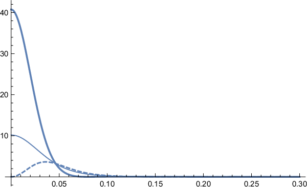
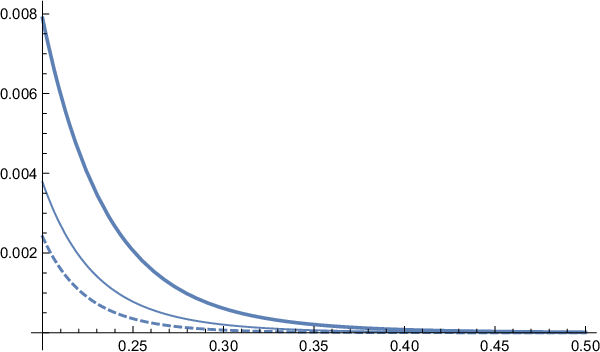
In view of this, it is not surprising that, in spite of the fact the kinematical function $K_{n}$ is quite large, the $S_{n\ell}$ factors are small:

S_{n\ell}=\left(\begin{array}[]{cccc}n&K(n)&S(S(n))&S(P(n))\\ \hline\cr 1&12.2&0.0424184&-\\ 2&101.9&0.00493614&0.000617041\\ \end{array}\right)

(87)

Thus using Eq. (85) we find

\sigma_{n\ell}=\{2.567,0.298,0.036\}\times 10^{-46}\mbox{cm}^{2}\left(\frac{g_{ae}}{0.024}\right)^{2}\left(\frac{m_{a}}{5\mbox{eV}}\right)^{2}

The total cross section is

\sigma=\sum_{n\ell}\sigma_{n\ell}=8.36\times 10^{-44}\mbox{cm}^{2}\left(\frac{g_{ae}}{0.024}\right)^{2}\left(\frac{m_{a}}{5\mbox{eV}}\right)^{2}

(88)

This cross section scaled to $m_{a}=5$ keV becomes $8.36\times 10^{-38}\mbox{cm}^{2}$ which between the values $10^{-36}\mbox{cm}^{2}$ (DFSZ) and $10^{-41}\mbox{cm}^{2}$ (KSVZ) reported by CUORE Cuore Collaboration 2013.

X.5 Some results regarding the rates for atomic ionization

Using now the 14.4 keV flux given by Eq. (71)) and $N_{A}=4\times 10^{27}$ as above we find:

i) For the iodine component:

R_{n,\ell}=\{0.337,2.810,0.016,0.503,0.830,0.003,0.194,0.340,0.082\}\times 10^{2}\mbox{per t-y}\left(\frac{m_{a}}{5\mbox{eV}}\right)^{4}\left(\frac{g_{ae}}{0.024}\right)^{2}

(89)

in the same order as in Eq, (86).

ii) For the Na component

R_{n,\ell}=\{1.575,0.182,0.022\}\mbox{per t-y}\left(\frac{m_{a}}{5\mbox{eV}}\right)^{4}\left(\frac{g_{ae}}{0.024}\right)^{2}

(90)

The obtained rates depend on the atomic wave function and in particular the form factor of the orbit involving the ejected electron. We have seen that a great suppression of the form occur, if the axion energy is high, e,g, 5 MeV. The same thing happens in the case of a 14,4 keV axion for a small $Z$ atom, since again, due to the small binding, the form factor is suppressed due large momentum transfer, see Fig. 8. Thus, for the Iodine atom, as well as others with nearby $Z$ and the 14.4 keV energy, we have a favorable situation. One can write for the dominant contributions:

R_{n,\ell}=\{0.337,2.810,0.503,0.829,0.340\}\times 10^{2}\mbox{per t-y}\left(\frac{m_{a}}{5\mbox{eV}}\right)^{4}\left(\frac{g_{ae}}{0.024}\right)^{2}

(91)

in the order $2S,\,2P,\,3P,\,3D,\mbox{ and }4D$ for the orbits.
We notice the dramatic dependence of the event rate on the axion mass. Deceasing the axion mass by a factor of 5 will lead to a reduction of the rate by 3 orders of magnitude and make it un-observable, an increase by the same factor makes one wonder how come such an axion has not already been seen.

XI Concluding remarks

In the present work we studied various axion induced nuclear and atomic processes, assuming an axion mass of 5 eV.

In the case of the nuclear processes we considered the mono-energetic axion source of 5.5 MeV. The obtained nuclear cross sections were found to be reasonable, but the obtained rates were very small mainly due to the small flux on the earth of such axions, obtained with the Borexino detector Bellini et al. 2012b. So, such processes are doomed to be non detectable for axion masses in the few eV range. Had the mass of the axion been in the keV region, such processes would become detectable with rates as given by Fig. 7 and, in particular, by Eqs (60) and (61). We have seen, however, that such masses are excluded by astrophysical data. For lower axion masses in the subkeV region, e.g. the value of $m_{a}=0.25$ keV, a model dependent limit extracted by the CUORE experiment Cuore Collaboration 2013, the obtained total excitation and photoproduction rates in the case of NaI target become $R\approx 6\times 10^{-3}$ and $R_{coh}\approx 10^{-5}\mbox{(t-y)}^{-1}$ respectively, exceedingly difficult to detect.

In the case of atomic experiments, with inner electron binding energies in the keV region, we found appropriate and we used the 14.4 keV ⁵⁷Fe axion source. In this case we find sizable rates, e.g.:
i) Axion induced photoproduction. We get the rate given by Eq. (80) for directly producing X-rays with energy equal to the axion energy $E_{a}$ . Smaller rates are expected from the excited states with about the same energy. This is independent of the details of the structure of the atom. For $m_{a}=5$ eV axions ( $f_{a}=1.2\times 10^{6}$ GeV) this leads to a rate $R\approx 2.50\mbox{ events per (t-y)}$ in the case of NaI target, assuming a coupling $g_{ae}=0.024$ .
ii) Electron ejection from the atom. In this case we find sizable rates for ejecting an electron from the relevant orbits of the Iodine, given by Eq. (91), the maximum being 280 events per t-y for $m_{a}=5$ eV ( $f_{a}=1.2\times 10^{6}$ GeV), again for $g_{ae}=0.024$ , coming from the $n=2,\ell=1$ orbit, and slightly smaller rates from some of the other orbits. Much smaller rates are expected for the Na component.

Experiments like those discussed above have already been done by CUORE-Te Cuore Collaboration 2013 and others Li et al. 2016, Derbin et al. 2011b. As given in Eq.(69), the 14.4 keV axion with the rate larger than $R=2\times 10^{5}(t-y)^{-1}(m_{a}<19$ eV DFSZ) has been excluded Cuore Collaboration 2013. Then, axions in the region of $R=(10^{2}-10^{4})(t-y)^{-1}$ , i.e. $m_{a}=5-10$ eV, $g_{ae}=0.024$ , are very interesting and their detection in the case of atomic excitations is quite realistic, by improving detector sensitivities by a few orders of magnitude.

If that is the case, we expect a very interesting axion signature, i.e. a signal consisting of the detection of the primarily produced electrons from each orbit as well as the detection of the X-rays or Auger electrons produced, when the created hole is filled by the de-excitation of the atom. The relevant rates depend, of course, on the assumed value of the elementary coupling $g_{ae}$ , which is not really known.

XII Appendix: The formalism of the axion electron cross section from bound orbits

The axion electron scattering cross section for relativistic axions is given by

d\sigma=\sigma_{0}\int{\cal M}(k^{2})^{2}\frac{1}{2E_{a}}\frac{d{\bf p}_{e}^{3}}{(2\pi)^{3}}\frac{d{\bf p}_{A}^{3}}{(2\pi)^{3}}(2\pi)\delta(E_{a}+\epsilon_{b}-T)(2\pi)^{3}\delta({\bf p}_{a}-{\bf p}_{A}-{\bf p}_{e})

(92)

where ${\cal M}(k^{2})$ is the invariant amplitude, which depends on the momentum transfer, ${\bf p}_{e}$ and $T$ are the momentum and the energy of the outgoing electron and ${\bf p}_{A}$ of the atom, $\epsilon_{b}$ is the binding energy of the electron in the target. $E_{a}$ is the energy of the axion, normally being introduced as a normalization of the scalar field. We have neglected the energy of the outgoing atom. Thus integrating over ${\bf p}_{A}$ with the use of the momentum conserving $\delta$ function we obtain

\sigma=\sigma_{0}\frac{1}{2}\frac{1}{(2\pi)^{2}}4\pi S=\frac{1}{2\pi}S,\,S=\frac{1}{4\pi}\int{\cal M}(k^{2})^{2}\frac{1}{E_{a}}d{\bf p}_{e}^{3}\delta(E_{a}+\epsilon_{b}-T)

(93)

Let us begin with the discussion of ${\cal M}(k^{2})^{2}$ . The relevant matrix element (ME) involving the initial bound electron and the outgoing plane wave electron is given by:

\mbox{ME}=\int\psi_{n\ell m}({\bf r})e^{i{\bf q\cdot{\bf r}}}\langle\frac{1}{2}m_{s}|\mbox{\boldmath$\sigma$}\cdot{\bf q}|\frac{1}{2}m_{s}^{\prime}\rangle\frac{1}{(2\pi)^{3/2}}e^{-i{\bf p_{e}\cdot{\bf r}}}=\phi_{n\ell m}({\bf k})\langle\frac{1}{2}m_{s}|\mbox{\boldmath$\sigma$}\cdot{\bf q}|\frac{1}{2}m_{s}^{\prime}\rangle,\,{\bf k}={\bf q}-{\bf p}_{e}

(94)

Where $\phi_{n\ell m}({\bf k})$ is the initial electron bound wave function in momentum space. The last term involves the axion electron interaction.We thus find that transition probability averaging over the initial m-substates and summing over the final ones becomes:

\frac{1}{(2j+1)}\sum_{m,m_{\ell},m_{s}.m_{s}^{\prime}}\langle\ell m_{\ell},\frac{1}{2}m_{s}|jm\rangle^{2}\mbox{ME}^{2}=|\phi_{n\ell m}({\bf k})|^{2}\langle\frac{1}{2}\sum_{m_{s},m_{s}^{\prime}}\frac{1}{2}m_{s}|\mbox{\boldmath$\sigma$}\cdot{\bf q}|\frac{1}{2}m_{s}^{\prime}\rangle^{2}

(95)

The last result was obtained using the properties of the Clebcsh-Gordan coefficients.The last matrix element can easily be evaluated yielding $q^{2}\approx E_{a}^{2}$ We thus find

S=\frac{1}{4\pi}\int|\phi_{n\ell m}({\bf k})|^{2}E_{a}d{\bf p}_{e}^{3}\delta(E_{a}+\epsilon_{b}-T)

(96)

We will specialize it in the case of 14.4 keV axion. In this case the outgoing electron is non relativistic $T=p_{e}^{2}/(2m_{e})$ , with the use of $\delta$ function we get $p_{e}=\sqrt{2m_{e}(E_{a}+\epsilon_{b})}$ , which is much larger than the axion momentum. So $k\approx p_{e}$ . So after the integration over the angles we get:

S=\left(\phi_{n\ell m}(\sqrt{2m_{e}(E_{a}+\epsilon_{b})})\right)^{2}E_{a}m_{e}\sqrt{2m_{e}(E_{a}+\epsilon_{b})}

(97)

At this point we recall that the bound state wave function can be written as $\phi_{n\ell}(a,k)$ , where $k$ is the momentum and $a=\frac{\alpha Zm_{e}}{n}$ . We prefer to write it in dimensionless form and write is as

F_{n\ell}(a,k)=a^{3}\phi^{2}_{n\ell}(a,k)\Rightarrow S=F_{n\ell}K_{n},\,K_{n}=n^{3}\frac{1}{(\alpha Z)^{3}}\frac{E_{a}}{m_{e}}\sqrt{2\left(\frac{E_{a}+\epsilon_{b}(n)}{m_{e}}\right)}

(98)

A compensating $1/a^{3}$ factor has been introduced in the kinematical portion of Eq, (97). This way both $F_{n\ell}$ and $K_{n}$ are dimensionless.

In the case of the 5.5 MeV axion we proceed in an analogous way. Now the binding becomes irrelevant and the outgoing electron caries all the energy, Its momentum however is $\sqrt{E_{a}(E_{a}+2m_{e})}$ , approximately the same with the axion momentum. So the angular integral is quite complicated and we made the simplifying assumption $k=\sqrt{q^{2}+p_{e}^{2}}$ Now

K_{n}=n^{3}\frac{1}{(\alpha Z)^{3}}\left(\frac{E_{a}}{m_{e}}\right)^{3}

(99)

As expected $K_{n}$ becomes large, but the form factor $F_{n\ell}(a,k)$ at this high momentum transfer is tiny, so that the cross section becomes negligibly small.

The relevant for factors employed are given below:

F_{1s}=\frac{128a^{8}(a-k)^{2}(a+k)^{2}}{\pi\left(a^{2}+k^{2}\right)^{6}},\,F_{0p}=\frac{512a^{10}k^{2}}{3\pi\left(a^{2}+k^{2}\right)^{6}},\,F_{2s}=\frac{32a^{8}\left(3a^{4}-10a^{2}k^{2}+3k^{4}\right)^{2}}{\pi\left(a^{2}+k^{2}\right)^{8}}

F_{1p}=\frac{1024a^{10}k^{2}(a-k)^{2}(a+k)^{2}}{\pi\left(a^{2}+k^{2}\right)^{8}},\,F_{0d}=\frac{4096a^{12}k^{4}}{5\pi\left(a^{2}+k^{2}\right)^{8}},\,F_{3s}=\frac{512a^{8}\left(a^{6}-7a^{4}k^{2}+7a^{2}k^{4}-k^{6}\right)^{2}}{\pi\left(a^{2}+k^{2}\right)^{10}}

F_{2p}=\frac{2048a^{10}k^{2}\left(5a^{4}-14a^{2}k^{2}+5k^{4}\right)^{2}}{15\pi\left(a^{2}+k^{2}\right)^{10}},\,F_{1d}=\frac{32768a^{12}k^{4}\left(a^{2}-k^{2}\right)^{2}}{5\pi\left(a^{2}+k^{2}\right)^{10}},\,F_{0g}=\frac{131072a^{14}k^{6}}{35\pi\left(a^{2}+k^{2}\right)^{10}}

Acknowledgments: J. D. V. would like to thank Georg Raffelt for his help in getting the axion mass dependence of the 14.4 keV axion solar flux.

References

Peccei and Quinn (1977) R. Peccei and H. Quinn, Phys. Rev. Lett 38, 1440 (1977).
Weinberg (1978) S. Weinberg, Phys. Rev. Lett. 40, 223 (1978).
Wilczek (1978) F. Wilczek, Phys. Rev. Lett. 40, 279 (1978).
Kim (1979) J. E. Kim, Phys. Rev. Lett. 43, 137 (1979).
Shifman et al. (1980) M. A. Shifman, A. Vainshtein, and V. I. Zakharov, Nuc. Phys. B 166, 493 (1980).
Dine et al. (1981) M. Dine, W. Fischler, and M. Srednicki, Phys. Lett. B 104, 199 (1981).
Zhitnisky (1980) A. Zhitnisky, Sov. J. Nuc. Phys. 31, 260 (1980), in Russian.
Abbott and Sikivie (1983) L. F. Abbott and P. Sikivie, Phys. Lett. B120, 133 (1983).
Dine and Fischler (1983) M. Dine and W. Fischler, Phys. Lett. B120, 137 (1983).
Preskill et al. (1983) J. Preskill, M. B. Wise, and F. Wilczek, Phys. Lett. B120, 127 (1983).
Asztalos et al. (2010) S. J. Asztalos et al., Phys. Rev. Lett. 104, 041301 (2010), the ADMX Collaboration, arXiv:0910.5914 (astro-ph.CO).
Duffy et al. (2005) L. Duffy et al., Phys. Rev. Lett. 95, 09134 (2005), for the ADMX Collaboration.
Wagner et al. (2010) A. Wagner et al., Phys. Rev. Lett. 105, 171801 (2010), for the ADMX collaboration; arXiv:1007.3766 (astro-ph.CO).
Irastorza and Garca (2012) I. G. Irastorza and J. A. Garca, JCAP 1210, 022 (2012), arXiv:1007.3766 (astro-ph.IM).
(15) T. M. Shokair, J. Root, K. Bibber, et al., international Journal of Modern Physics A, arXiv:1405.3685 [physics.ins-det].
Marsh (2016) D. J. E. Marsh, Phys. Rep. D 643, 1 (2016).
Kaplan (1985) D. B. Kaplan, Nuc. Phys. B 260, 215 (1985).
Turner (1997) M. S. Turner, Phys. Rev. Lett. 60, 1797 (1997).
Carenza et al. (2019) P. Carenza et al., JCAP 10, 016 (2019), arXiv:1906.11844 [hep-ph].
Borisov and Grishina (1996) A. V. Borisov and V. Y. Grishina, JETP 83, 868 (1996).
Derbin et al. (2011a) A. Derbin, A. Kayunov, V. Muratova, D. Semenov, and E. Unzhakov, Phys. Rev. D. 83, 023505 (2011a).
Primakoff (1951) H. Primakoff, Phys. Rev 81, 899 (1951).
Zioutas et al. (2005) K. Zioutas et al. (The CAST Collaboration), Phys. Rev. Lett. 94, 1213811 (2005).
Sierra et al. (2021) D. A. Sierra, V. De Romeri, L. J. Flores, and D. Papoulias, JHEP 03, 294 (2021), arXiv: 2010.15712 [hep-ph].
deNiverville et al. (2021) P. deNiverville, Hye-Sung Lee, and Young-Min Lee, Phys. Rev. D 103, 075006 (2021), arXiv:2011.03276 [hep-ph].
Andriamonje et al. (2009) S. Andriamonje et al. (The CAST collaboration), J. Cosmol. Astropart. Phys. 12, 002 (2009).
Arik et al. (2014) M. Arik et al. (The CAST collaboration), Phys. Rev. Lett. 112, 091302 (2014).
Alessandria et al. (2013) F. Alessandria et al., J. Cosmol. Astropart. Phys. 05, 007 (2013).
Namba (2007) T. Namba, Phys. Lett. B 645, 398 (2007).
Arnaboldi et al. (2004) C. Arnaboldi et al. (The CUORE collaboration), Nucl. Instrum. Meth. A 518, 775 (2004).
(31) R. Ardito et al (CUORE Collaboration), CUORE: A Cryogenic Underground Observatory for Rare Events, arXiv:hep-ex/0501010, (2005).
Artusa et al. (2015) D. R. Artusa et al. (The CUORE collaboration), Adv. High Ener. Phys. 2015, 879871 (2015), http://dx.doi.org/10.1155/2015/870871.
(33) C. Alduino et al., (The CUORE Collaboration) arXiv:1710.07988, Submitted to Phys. Rev. Lett.
Cuore Collaboration (2013) Cuore Collaboration (The CUORE collaboration), JCAP 05, 007 (2013).
Abgrall et al. (2016) N. Abgrall et al. (The Majorana Collaboration), Nucl. Instr. Meth. Phys. Res. A 828, 22 (2016).
Agostini et al. (2013) M. Agostini et al. (The GERDA Collaboration), Phys. Rev. Lett. 111, 122583 (2013).
Li et al. (2016) D. Li, R. Creswick, F.T. Avignone III, and Y. Wang, JCAP 02, 031 (2016), arXiv:1512.01298 (astro-ph.CO).
F.T. Avignone III (2009) F.T. Avignone III, Journal of Physics 173, 012015 (2009).
Aalseth et al. (2011) C. Aalseth et al., Phys. Rev. Lett. 106, 131301 (2011), coGeNT collaboration arXiv:10002.4703 [astro-ph.CO].
F.T. Avignone III et al. (2018) F.T. Avignone III, R. Creswick, J. Vergados, P. Pirinen, P. Srivastava, and J. Suhonen, JCAP 01, 021 (2018).
Bellini et al. (2012a) G. Bellini et al. (The Borexino Collaboration), Phys. Rev. D 85, 092003 (2012a), arXiv:1203.6258 [hep-ex].
Andriamonje et al. (2010) S. Andriamonje et al. (The CAST collaboration), JCAP 1003, 832 (2010), arXiv:0904.2103 [hep-ex].
Bhusal et al. (2020) A. Bhusal, N. Houston, and T. Li (2020), searching for solar axions at the Sudbury Neutrino Observatory, arXiv:2004.02733 [Hep-ph].
Patrignani et al. (2016) C. Patrignani et al. (Particle Data Group), Chin. Phys. C 40, 100001 (2016).
(45) M. Gorghetto and G. Villadoro, Topological Susceptibility and QCD Axion Mass: QED and NNLO corrections, arXiv:1812.01008 [hep-ph].
Bali et al. (2012) G. Bali et al., Phys. Rev. Lett. 108, 222001 (2012).
Li and Thomas (2016) J. Li and A. W. Thomas, Nuc. Phys.B 906, 60 (2016), arXiv:1506.03560 [hep-ph].
(48) The Strange Spin of the Nucleon, J. Ellis and M. Karliner, hep-ph/9501280.
(49) S Pate (for the MicroBooNE Collaboration), Progress On Neutrino-Proton Neutral-Current Scattering In MicroBooNE, arXiv:1701.04483 [nucl-ex].
Ejiri (2005) H. Ejiri, J. Phys. Soc. Jpn. 74, 2181 (2005).
Ejiri et al. (2019) H. Ejiri, J. Suhonen, and K. Zuber, Phys. Rep. 797, 1 (2019).
Ejiri and Zuber (2017) H. Ejiri and K. J. Zuber, Nucl. Part. Phys. G 43, 045201 (2017).
Ejiri and Elliott (2014) H. Ejiri and S. R. Elliott, Phys. Rev. C 89, 055281 (2014).
Ejiri and Elliott (2017) H. Ejiri and S. R. Elliott, Phys. Rev. C 95, 055581 (2017).
Ericson and Rho (1972) M. Ericson and M. Rho, Phys. Rep. 5, 75 (1972).
Baer et al. (1975) H. W. Baer et al., Phys. Rev. C 12, 921 (1975).
Vergados et al. (2012) J. D. Vergados, H. Ejiri, and F. Simkovic, Rep. Prog. Phys. 75, 106301 (2012).
Caurier et al. (2005) E. Caurier, Martinez-Pinedo, F. Nowacki, A. Poves, and A. Zuker, Rev. Mod. Phys. 77, 427 (2005).
Klos and et al (2013) P. Klos and et al, Rev. Rev. D 88, 083516 (2013).
Caurier et al. (2008) E. Caurier, Martinez-Pinedo, F. Nowacki, and A. Poves, Rev. Lett. 100, 052503 (2008).
Ressell and Dean (1997) M. T. Ressell and D. J. Dean, Rev. Rev. C 56, 535 (1997).
Hashizume (2011) A. Hashizume, Nuclear Data Sheets 112, 1647 (2011).
Divari et al. (2000) P. C. Divari, T. S. Kosmas, J. D. Vergados, and L. D. Skouras, Phys. Rev. C 61, 054612 (2000).
Peccei (1996) R. D. Peccei, J. Korean Phys. Soc. 29, S199 (1996), hep-ph/9606475.
Bellini et al. (2012b) G. Bellini et al., Phys. Rev. D 85, 092003 (2012b), arXiv:1203.6258 [hep-ex].
Bernabei et al. (1999) R. Bernabei et al., Phys. Lett. B 458, 448 (1999).
Bernabei et al. (2008) R. Bernabei et al., Nucl. Instr. and Meth.A 592, 297 (2008).
Bernabei et al. (2018) R. Bernabei et al. (DAMA LIBRA Phase 2), Nuc. Phys and Atom. Energ. 19.4, 387 (2018).
Kim et al. (2012) S. C. Kim et al. (DAMA LIBRA Phase 2), Phys. Rev. Lett. 108, 181381 (2012).
G. G. Raffelt (2008) G. G. Raffelt, Lect. Notes Phys. 741, 51 (2008), arXiv hep-ph/ 0611350.
M. Krcmar et al. (2001) M. Krcmar et al., Phys. Rev. D 64, 115016 (2001).
A. V. Derbin et al. (2005) A. V. Derbin et al., JETP Lett. 81, 365 (2005).
P. Belli et al. (2008) P. Belli et al., Nucl. Phys. A 806, 388 (2008).
Srednicki (1985) M. Srednicki, Nucl. Phys. B 260, 689 (1985).
di Cortona et al. (2016) G. G. di Cortona, E. Hardy, J. P. Vega, and G. Villadoro, JHEP 01, 034 (2016), arXiv:1511.02867, (hep-ph), (hep-ex), (hep-lat).
Ringwald and Saikawa (2016) A. Ringwald and K. Saikawa, Phys. Rev. D 93, 085031 (2016), arXiv:1512.06436 [hep-ph].
Derbin et al. (2011b) A. V. Derbin, V. N. Muratova, D. A. Semenov, and E. V. Unzhakov, Phys. Atom. Nuclei 74, 596 (2011b).
Abe et al. (2021) T. Abe, K. Hamaguchi, and N. Nagata, Phys. Lett. B 815, 136174 (2021), arXiv:2012.02508 [hep-ph].