Rory Mitchell, Joshua Cooper, Eibe Frank and Geoffrey Holmes
Sampling Permutations for Shapley Value Estimation
Abstract
Game-theoretic attribution techniques based on Shapley values are used to interpret black-box machine learning models, but their exact calculation is generally NP-hard, requiring approximation methods for non-trivial models. As the computation of Shapley values can be expressed as a summation over a set of permutations, a common approach is to sample a subset of these permutations for approximation. Unfortunately, standard Monte Carlo sampling methods can exhibit slow convergence, and more sophisticated quasi-Monte Carlo methods have not yet been applied to the space of permutations. To address this, we investigate new approaches based on two classes of approximation methods and compare them empirically. First, we demonstrate quadrature techniques in a RKHS containing functions of permutations, using the Mallows kernel in combination with kernel herding and sequential Bayesian quadrature. The RKHS perspective also leads to quasi-Monte Carlo type error bounds, with a tractable discrepancy measure defined on permutations. Second, we exploit connections between the hypersphere and permutations to create practical algorithms for generating permutation samples with good properties. Experiments show the above techniques provide significant improvements for Shapley value estimates over existing methods, converging to a smaller RMSE in the same number of model evaluations.
keywords
Interpretability, quasi-Monte Carlo, Shapley values1 Introduction
The seminal work of Shapley 1953 introduces an axiomatic attribution of collaborative game outcomes among coalitions of participating players. Aside from their original applications in economics, Shapley values are popular in machine learning (Cohen et al. 2007; Strumbelj and Kononenko 2010; Štrumbelj and Kononenko 2014; Lundberg and Lee 2017) because the assignment of feature relevance to model outputs is structured according to axioms consistent with human notions of attribution. In the machine learning context, each feature is treated as a player participating in the prediction provided by a machine learning model and the prediction is considered the outcome of the game. Feature attributions via Shapley values provide valuable insight into the output of complex models that are otherwise difficult to interpret.
Exact computation of Shapley values is known to be NP-hard in general (Deng and Papadimitriou 1994) and approximations based on sampling have been proposed by several authors: Mann and Shapley 1960; Owen 1972; Castro et al. 2009; Maleki 2015; Castro et al. 2017. In particular, a simple Monte Carlo estimate for the Shapley value is obtained by sampling from a uniform distribution of permutations. The extensively developed quasi-Monte Carlo theory for integration on the unit cube shows that careful selection of samples can improve convergence significantly over random sampling, but these results do not extend to the space of permutations. Here, our goal is to better characterise ‘good’ sample sets for this unique approximation problem, and to develop tractable methods of obtaining these samples, reducing computation time for high-quality approximations of Shapley values. Crucially, we observe that sample evaluations, in this context corresponding to evaluations of machine learning models, dominate the execution time of approximations. Due to the high cost of each sample evaluation, considerable computational effort can be justified in finding such sample sets.
In Section 3, we define a reproducing kernel Hilbert space (RKHS) with several possible kernels over permutations by exploiting the direct connection between Shapley values and permutations. Using these kernels, we apply kernel herding, and sequential Bayesian quadrature algorithms to estimate Shapley values. In particular, we observe that kernel herding, in conjunction with the universal Mallows kernel, leads to an explicit convergence rate of as compared to for ordinary Monte Carlo. An outcome of our investigation into kernels is a quasi-Monte Carlo type error bound, with a tractable discrepancy formula.
In Section 4, we describe another family of methods for efficiently sampling Shapley values, utilising a convenient isomorphism between the symmetric group and points on the hypersphere . These methods are motivated by the relative ease of selecting well-spaced points on the sphere, as compared to the discrete space of permutations. We develop two new sampling methods, termed orthogonal spherical codes and Sobol permutations, that select high-quality samples by choosing points well-distributed on .
Our empirical evaluation in Section 5 examines the performance of the above methods compared to existing methods on a range of practical machine learning models, tracking the reduction in mean squared error against exactly calculated Shapley values for boosted decision trees and considering empirical estimates of variance in the case of convolutional neural networks. Additionally, we evaluate explicit measures of discrepancy (in the quasi-Monte Carlo sense) for the sample sets generated by our algorithms. This evaluation of discrepancy for the generated samples of permutations may be of broader interest, as quasi-Monte Carlo error bounds based on discrepancy apply to any statistics of functions of permutations and not just Shapley values.
In summary, the contributions of this work are:
- •
The characterisation of the Shapley value approximation problem in terms of reproducing kernel Hilbert spaces.
- •
Connecting the Shapley value approximation problem to existing quasi-Monte Carlo approaches, using kernels and connections between the hypersphere and symmetric group.
- •
Experimental evaluation of these methods in terms of discrepancy, and the error of Shapley value approximations on tabular and image datasets.
2 Background and Related Work
We first introduce some common notation for permutations and provide the formal definition of Shapley values. Then, we briefly review the literature for existing techniques for approximating Shapley values.
2.1 Notation
We refer to the symmetric group of permutations of elements as . We reserve the use of to refer to the number of samples. The permutation assigns rank to element by . For example, given the permutation written in one-line notation
and the list of items
the items are reordered such that occupies the coordinate
and the inverse is
An inversion is a pair of elements in the permutation such that and . The identity permutation,
contains 0 inversions, and its reverse
contains the maximum number of inversions, .
2.2 Shapley Values
Shapley values (Shapley 1953) provide a mechanism to distribute the proceeds of a cooperative game among the members of the winning coalition by measuring marginal contribution to the final outcome. The Shapley value for coalition member is defined as
| (1) |
where is a partial coalition, is the grand coalition (consisting of all members), and is the so-called “characteristic function” that is assumed to return the proceeds (i.e., value) obtained by any coalition.
The Shapley value function may also be conveniently expressed in terms of permutations
| (2) |
where represents the set of players ranked lower than in the ordering . To see the equivalence between (1) and (2), consider that is the number of unique orderings the members of can join the coalition before , and is the number of unique orderings the remaining members can join the coalition after . The Shapley value is unique and has the following desirable properties:
- 1.
Efficiency: The sum of Shapley values for each coalition member is the value of the grand coalition .
- 2.
Symmetry: If, , then If two players have the same marginal effect on each coalition, their Shapley values are the same.
- 3.
Linearity: . The Shapley values of sums of games are the sum of the Shapley values of the respective games.
- 4.
Dummy: If, , then . The coalition member whose marginal impact is always zero has a Shapley value of zero.
Evaluation of the Shapley value is known to be NP-hard in general (Deng and Papadimitriou 1994) but may be approximated by sampling terms from the sum of either Equation 1 or Equation 2. This paper focuses on techniques for approximating Equation 2 via carefully chosen samples of permutations. We discuss characteristic functions that arise in the context of machine learning models, with the goal of attributing predictions to input features.
Shapley values have been used as a feature attribution method for machine learning in many prior works (Cohen et al. 2007; Strumbelj and Kononenko 2010; Štrumbelj and Kononenko 2014; Lundberg and Lee 2017). In the terminology of supervised learning, we have some learned model that maps a vector of features to a prediction . In this context, the Shapley values will be used to evaluate the weighted marginal contribution of features to the output of the predictive model. The value of the characteristic function is assumed to be given by , and the grand coalition is given by the full set of features. In a partial coalition, only some of the features are considered “active” and their values made available to the model to obtain a prediction. Applying the characteristic function for partial coalitions requires the definition of , where the input features are perturbed in some way according to the active subset . A taxonomy of possible approaches is given in Covert et al. 2020.
2.3 Monte Carlo
An obvious Shapley value approximation is the simple Monte Carlo estimator,
| (3) |
for a uniform sample of permutations of size . Monte Carlo techniques were used to solve electoral college voting games in Mann and Shapley 1960, and a more general analysis is given in Castro et al. 2009. Equation 3 is an unbiased estimator that converges asymptotically at a rate of according to the Central Limit Theorem.
From a practical implementation perspective, note that a single sample of permutations can be used to evaluate for all features . For each permutation of length , first evaluate the empty set , then walk through the permutation, incrementing and evaluating , yielding evaluations of that are used to construct marginal contributions for each feature. is not evaluated, but reused from the previous function evaluation, providing a factor of two improvement over the naive approach.
2.4 Antithetic Sampling
Antithetic sampling is a variance reduction technique for Monte Carlo integration where samples are taken as correlated pairs instead of standard i.i.d. samples. The antithetic Monte Carlo estimate (see Rubinstein and Kroese 2016) is
with variance given by
| (4) |
such that if and are negatively correlated, the variance is reduced. A common choice for sampling on the unit cube is with . Antithetic sampling for functions of permutations is discussed in Lomeli et al. 2019, with a simple strategy being to take permutations and their reverse. We implement this sampling strategy in our experiments with antithetic sampling.
2.5 Multilinear Extension
Another Shapley value approximation method is the multilinear extension of Owen 1972. The sum over feature subsets from (1) can be represented equivalently as an integral by introducing a random variable for feature subsets. The Shapley value is calculated as
| (5) |
where
and is a random subset of features, excluding , where each feature has probability of being selected. is estimated with samples. In our experiments, we implement a version of the multilinear extension algorithm using the trapezoid rule to sample at fixed intervals. A form of this algorithm incorporating antithetic sampling is also presented in Okhrati and Lipani 2020, by rewriting Equation 5 as
where the sample set is used to estimate and the ‘inverse set’, , is used to estimate . In Section 5, we include experiments for the multilinear extension method both with and without antithetic sampling.
2.6 Stratified Sampling
Another common variance reduction technique is stratified sampling, where the domain of interest is divided into mutually exclusive subregions, an estimate is obtained for each subregion independently, and the estimates are combined to obtain the final estimate. For integral in domain , separable into non-overlapping regions where and , the basic stratified sampling estimator is
where for and (see Owen 2003). The stratum size can be chosen with the Neyman allocation (Neyman 1934) if estimates of the variance in each region are known. The stratified sampling method was first applied to Shapley value estimation by Maleki 2015, then improved by Castro et al. 2017. We implement the version in Castro et al. 2017, where strata are considered for all and , where is the subset of marginal contributions with feature at position .
This concludes discussion of existing work; the next sections introduce the primary contributions of this paper.
3 Kernel Methods
A majority of Monte Carlo integration work deals with continuous functions on , where the distribution of samples is well defined. In the space of permutations, distances between samples are not implicitly defined, so we impose a similarity metric via a kernel and select samples with good distributions relative to these kernels.
Given a positive definite kernel over some input space , there is an embedding of elements of into a Hilbert space , where the kernel computes an inner product given . Hilbert spaces associated with a kernel are known as reproducing kernel Hilbert spaces (RKHS). Kernels are used extensively in machine learning for learning relations between arbitrary structured data. In this paper, we use kernels over permutations to develop a notion of the quality of finite point sets for the Shapley value estimation problem, and for the optimisation of such point sets. For this task, we investigate three established kernels over permutations: the Kendall, Mallows, and Spearman kernels.
The Kendall and Mallows kernels are defined in Jiao and Vert 2015. Given two permutations and of the same length, both kernels are based on the number of concordant and discordant pairs between the permutations:
Assuming the length of the permutation is , the Kendall kernel, corresponding to the well-known Kendall tau correlation coefficient (Kendall 1938), is
The Mallows kernel, for , is defined as
Here, the Mallows kernel differs slightly from that of Jiao and Vert 2015. We normalise the term relative to , allowing a consistent selection of the parameter across permutations of different length.
While the straightforward implementation of Kendall and Mallows kernels is of order , a variant based on merge-sort is given by Knight 1966.
Note that can also be expressed in terms of a feature map of elements,
so that
The Mallows kernel corresponds to a more complicated feature map, although still finite dimensional, given in Mania et al. 2018.
We also define a third kernel based on Spearman’s . The (unnormalised) Spearman rank distance,
is a semimetric of negative type (Diaconis 1988), therefore we can exploit the relationship between semimetrics of negative type and kernels from Sejdinovic et al. 2013 to obtain a valid kernel. Writing using vector notation as , we have
and the kernel’s feature map is trivially
Before introducing sampling algorithms, we derive an additional property for the above kernels: analytic formulas for their expected values at some fixed point and values drawn from a given probability distribution . The distribution of interest for approximating (2) is the uniform distribution . The expected value is straightforward to obtain for the Spearman and Kendall kernels:
The Mallows kernel is more difficult. Let be a random variable representing the number of inversions over all permutations of length . Its distribution is studied in Muir 1898, with probability generating function given as
There is no convenient form in terms of standard functions for its associated density function. From the probability generating function of , we obtain the moment generating function:
The quantity , where is the identity permutation, returns exactly the number of inversions in . Therefore, we have
The quantity is right-invariant in the sense that for (Diaconis 1988), so
We now describe two greedy algorithms for generating point sets improving on simple Monte Carlo—kernel herding and sequential Bayesian quadrature.
3.1 Kernel Herding
A greedy process called “kernel herding” for selecting (unweighted) quadrature samples in a reproducing kernel Hilbert space is proposed in Chen et al. 2010. The sample in kernel herding is given by
| (6) |
which can be interpreted as a greedy optimisation process selecting points for maximum separation, while also converging on the expected distribution . In the case of Shapley value estimation, the samples are permutations and is a uniform distribution with .
Kernel herding has time complexity for samples, assuming the argmax can be computed in time and is available. We have analytic formulas for from the previous section for the Spearman, Kendall, and Mallows kernels, and they give constant values depending only on the size of the permutation . We compute an approximation to the argmax in constant time by taking a fixed number of random samples at each iteration and retaining the one yielding the maximum.
If certain conditions are met, kernel herding converges at the rate , an improvement over for standard Monte Carlo sampling. According to Chen et al. 2010, this improved convergence rate is achieved if the RKHS is universal, and mild assumptions are satisfied by the argmax (it need not be exact). Of the Spearman, Kendall and Mallows kernels, only the Mallows kernel has the universal property (Mania et al. 2018).
Next, we describe a more sophisticated kernel-based algorithm generating weighted samples.
3.2 Sequential Bayesian Quadrature
Bayesian Quadrature (O’Hagan 1991; Rasmussen and Ghahramani 2003) (BQ) formulates the integration problem
as a Bayesian inference problem. Standard BQ imposes a Gaussian process prior on with zero mean and kernel function . A posterior distribution is inferred over conditioned on a set of points . This implies a distribution on with expected value
where is the vector of function evaluations at points , is the inverse of the kernel covariance matrix, and . Effectively, for an arbitrary set of points, Bayesian quadrature solves the linear system to obtain a reweighting of the sample evaluations, yielding the estimate
An advantage of the Bayesian approach is that uncertainty is propagated through to the final estimate. Its variance is given by
| (7) |
This variance estimate is used in Huszár and Duvenaud 2012 to develop sequential Bayesian quadrature (SBQ), a greedy algorithm selecting samples to minimise Equation 7. This procedure, summarised in Algorithm 1, is shown by Huszár and Duvenaud 2012 to be related to optimally weighted kernel herding. Note that the expectation term in (7) and Algorithm 1 is constant and closed-form for all kernels considered here.
SBQ has time complexity for samples if the argmin takes constant time, and an Cholesky update algorithm is used to form , adding one sample at a time. In general, exact minimisation of Equation 7 is not tractable, so as with kernel herding, we approximate the argmin by drawing a fixed number of random samples and choosing the one yielding the minimum variance.
3.3 Error Analysis in RKHS
Canonical error analysis of quasi Monte-Carlo quadrature is performed using the Koksma-Hlawka inequality (Hlawka 1961; Niederreiter 1992), decomposing error into a product of function variation and discrepancy of the sample set. We derive a version of this inequality for Shapley value approximation in terms of reproducing kernel Hilbert spaces. Our derivation mostly follows Hickernell 2000, with modification of standard integrals to weighted sums of functions on , allowing us to calculate discrepancies for point sets generated by kernel herding and SBQ with permutation kernels. The analysis is performed for the Mallows kernel, which is known to be a universal kernel (Mania et al. 2018).
Given a symmetric, positive definite kernel , we have a unique RKHS with inner product and norm , where the kernel reproduces functions by
Define error functional
where is a sample set of permutations and is the associated weight of sample . Because the Mallows kernel is a universal kernel, the bounded Shapley value component functions belong to . Given that is a continuous linear functional on and assuming that it is bounded, by the Riesz Representation Theorem, there is a function that is its representer: . Using the Cauchy-Schwarz inequality, the quadrature error is bounded by
where is the discrepancy of point set with weights and is the function variation. The quantity has an explicit formula. As the function is reproduced by the kernel, we have:
Then the discrepancy can be obtained, using the fact that , by
| (8) | ||||
It can be seen that kernel herding (Equation 6) greedily minimises with constant weights , by examining the reduction in obtained by the addition of a sample to . The kernel herding algorithm for sample is
Note that, since is right-invariant, the quantity does not depend on , so the argmax above is simply minimizing . On the other hand, denoting the identity permutation by , for a newly selected permutation sample :
where both equalities use right-invariance. Note that the first two summands in the last expression are constants (i.e., do not depend on the choice of ), so maximizing this quantity is the same as minimizing , i.e., the same as the kernel herding optimization subproblem.
Furthermore, we can show that Bayesian quadrature minimises squared discrepancy via optimisation of weights. Writing and switching to vector notation we have
where the first term is a constant not depending on . Taking the gradient with respect to , setting it to 0, and solving for , we obtain:
| (9) |
4 Sampling Permutations on
Kernel herding and sequential Bayesian quadrature directly reduce the discrepancy of the sampled permutations via greedy optimisation. We now describe two approaches to sampling permutations of length based on a relaxation to the Euclidean sphere , where the problem of selecting well-distributed samples is simplified. We describe a simple procedure for mapping points on the surface of this hypersphere to the nearest permutation, where the candidate nearest neighbours form the vertices of a Cayley graph inscribing the sphere. This representation provides a natural connection between distance metrics over permutations, such as Kendall’s tau and Spearman’s rho, and Euclidean space. We show that samples taken uniformly on the sphere result in a uniform distribution over permutations, and evaluate two unbiased sampling algorithms. Our approach is closely related to that of Plis et al. 2010, where an angular view of permutations is used to solve inference problems.
4.1 Spheres, Permutohedrons, and the Cayley Graph
Consider the projection of permutations as points in , where the -th coordinate is given by . These points form the vertices of a polytope known as the permutohedron (Guilbaud and Rosenstiehl 1963). The permutohedron is a dimensional object embedded in dimensional space, lying on the hyperplane given by
with normal vector
| (10) |
and inscribing the hypersphere lying on the hyperplane, defined by


Inverting the permutations at the vertices of the permutohedron gives a Cayley graph of the symmetric group with adjacent transpositions as the generating set. Figure 1 shows the Cayley graph for , whose vertices form a hexagon inscribing a circle on a hyperplane, and Figure 2 shows the Cayley graph of projected into three dimensions (its vertices lie on a hyperplane in four dimensions). Each vertex in the Cayley graph has neighbours, where each neighbour differs by exactly one adjacent transposition (one bubble-sort operation). Critically for our application, this graph has an interpretation in terms of distance metrics on permutations. The Kendall-tau distance is the graph distance in the vertices of this polytope, and Spearman distance is the squared Euclidean distance between two vertices (Thompson 1993). Additionally, the antipode of a permutation is its reverse permutation. With this intuition, we use the hypersphere as a continuous relaxation of the space of permutations, where selecting samples far apart on the hypersphere corresponds to sampling permutations far apart in the distance metrics of interest.
We now describe a process for sampling from the set of permutations inscribing . First, shift and scale the permutohedron to lie around the origin with radius . The transformation on vertex is given by
| (11) |
where is the mean vector of all permutations, and .
Now select some vector of dimension , say, uniformly at random from the surface of . Project onto the hyperplane in using the following matrix:
It is easily verifiable that this basis of row vectors is orthogonal to hyperplane normal . Normalising the row vectors of gives a transformation matrix used to project vector to the hyperplane by
so that
Given , find the closest permutation by maximising the inner product
| (12) |
This maximisation is simplified by noting that is always a reordering of the same constants ( is a scaled and shifted permutation). The inner product is therefore maximised by matching the largest element in against the largest element in , then proceeding to the second-largest, and so on. Thus the argmax is performed by finding the permutation corresponding to the order type of , which is order-isomorphic to the coordinates of . The output is a vertex on a scaled permutohedron — to get the corresponding point on the Cayley graph, undo the scale/shift of Eq. 11 to get a true permutation, then invert that permutation:
| (13) |
In fact, both Eq. 12 and 13 can be simplified via a routine argsort, defined by
such that
In other words, contains the indices of the elements of in sorted position.
Algorithm 2 describes the end-to-end process of sampling. We use the algorithm of Knuth 1997 for generating points uniformly at random on : sample from independent Gaussian random variables and normalise the resulting vector to have unit length. We now make the claim that Algorithm 2 is unbiased.
Theorem 1.
Algorithm 2 generates permutations uniformly at random, i.e., , from a uniform random sample on .
Proof.
The point from Algorithm 2, line 2, has multivariate normal distribution with mean 0 and covariance for some scalar and as the identity matrix. is an affine transformation of a multivariate normal and so has covariance
The matrix has the form
with all diagonal elements and off diagonal elements , and so is equicorrelated. Due to equicorrelation, has order type such that . In other words, all orderings of are equally likely. The function argsort implies an order-isomorphic bijection, that is, argsort returns a unique permutation for every unique ordering over its input. As every ordering of is equally likely, Algorithm 2 outputs permutations with ∎
Furthermore, Equation 12 associates a point on the surface of to the nearest permutation. This implies that there is a Voronoi cell on the same surface associated with each permutation , and a sample is associated with if it lands in its cell. Figure 3 shows the Voronoi cells on the hypersphere surface for , where the green points are equidistant from nearby permutations. A corollary of Theorem 1 is that these Voronoi cells must have equal measure, which is easily verified for .
4.2 Orthogonal Spherical Codes
Having established an order isomorphism , we consider selecting well-distributed points on . Our first approach, described in Algorithm 3, is to select dependent samples on from a basis of orthogonal vectors. Algorithm 3 uses the Gram-Schmidt process to incrementally generate a random basis, then converts each component and its reverse into permutations by the same mechanism as Algorithm 2. The cost of each additional sample is proportional to . This sampling method is related to orthogonal Monte Carlo techniques discussed in Choromanski et al. 2019. Writing , the Shapley value estimate for samples given by Algorithm 3 is
| (14) |
where are a set of correlated samples and is a multiple of .
Proposition 1.
is an unbiased estimator of .
Proof.
The Shapley value is equivalently expressed as an expectation over uniformly distributed permutations:
The distribution of permutations drawn as orthogonal samples is clearly symmetric, so for any two indices in a set of samples, and . As the estimator (14) is a sum, by the linearity of expectation
By Theorem 1, the random variable has a uniform distribution if its associated sample is drawn with uniform distribution. Let be a component of a random orthogonal basis. If the random basis is drawn with equal probability from the set of orthogonal matrices of order (i.e. with Haar distribution for the orthogonal group), then it follows that . The Gram-Schmidt process applied to a square matrix with elements as i.i.d. standard normal random variables yields a random orthogonal matrix with Haar distribution (Mezzadri 2006). Therefore
∎
The variance of the estimator (14) can be analysed similarly to the antithetic sampling of Section 2.4, extended to correlated random variables. By extension of the antithetic variance in Equation 4, we have
The variance is therefore minimised by selecting negatively correlated samples. Our experimental evaluation in Section 5 suggests that, for the domain of interest, orthogonal samples on the sphere are indeed strongly negatively correlated, and the resulting estimators are more accurate than standard Monte Carlo and antithetic sampling in all evaluations.
Samples from Algorithm 3 can also be considered as a type of spherical code. Spherical codes describe configurations of points on the unit sphere maximising the angle between any two points (see Conway et al. 1987). A spherical code gives the maximum number of points in dimension with minimum angle . The orthonormal basis and its antipodes trivially yield the optimal code .
From their relative positions on the Cayley graph we obtain bounds on the Kendall tau kernel from Section 3 for the samples of Algorithm 3. The angle between vertices of the Cayley graph is related to in that the maximum kernel value of 1 occurs for two permutations at angle 0 and the minimum kernel value of -1 occurs for a permutation and its reverse, separated by angle . As the angle between two points on increases from 0 to , the kernel for the nearest permutations decreases monotonically and linearly with the angle, aside from quantisation error. If the angle between two distinct points in our spherical codes is , we obtain via the map, , the permutations such that
with some small constant quantisation error . Figure 4 shows samples for the case. This is made precise in the following result. Note that the statement and its proof are in terms of and instead of their inverses (which label the vertices of the permutohedron in our convention), for simplicity; without this change, the meaning is the same, since and for any permutations , . First, let , so that the map maps the permutohedron to an isometric copy of centered at the origin in , the intersection of the unit sphere with the hyperplane orthogonal to .
Theorem 2.
Suppose . Then
and, if , then
Proof of the above can be found in Appendix A. Theorem 2 is a kind of converse to the so-called Rearrangement Inequality, which states that the maximum dot product between a vector and a vector consisting of any permutation of its coordinates is maximized when the permutation is the identity and minimized when it is the reverse identity. Here, we show what happens in between: as one varies from the identity to its reverse one adjacent transposition at a time, the dot product smoothly transitions from maximal to minimal, with some variability across permutations having the same number of inversions. Interestingly, we do not know if the above bound is the best possible. A quick calculation shows that, letting be an integer, the permutation
has , i.e, . However, admits inversions, whence .
Figure 5 shows the distribution of pairs of unique samples taken from random vectors, versus unique samples from an orthogonal basis, at . Samples corresponding to orthogonal vectors are tightly distributed around , and pairs corresponding to a vector and its antipodes are clustered at . Figure 6 plots the bounds from Theorem 2 relating the dot product of vectors on to the Kendall tau kernel at .


4.3 Sobol Sequences on the Sphere
We now describe another approach to sampling permutations via , based on standard quasi-Monte Carlo techniques. Low discrepancy point sets on the unit cube may be projected to via area preserving transformations. Such projections are discussed in depth in Brauchart and Dick 2012; Hardin et al. 2016, where they are observed to have good properties for numerical integration. Below we define transformations in terms of the inverse cumulative distribution of the generalised polar coordinate system and use transformed high-dimensional Sobol sequences to obtain well-distributed permutations.
In the generalised polar coordinate system of Blumenson 1960, a point on is defined by radius (here ) and angular coordinates , where range from and ranges from .
The polar coordinates on the sphere are independent and have probability density functions
and for :
where is the beta function. The above density function is obtained by normalising the formula for the surface area element of a hypersphere to integrate to 1 (Blumenson 1960). The cumulative distribution function for the polar coordinates is then
As per standard inverse transform sampling, we draw samples uniformly from the unit cube and project them to polar coordinates uniformly distributed on the sphere as . can be obtained quickly via a root finding algorithm, such as the bracketing method described in Press et al. 2007.
The points are generated using the Sobol sequence (Sobol’ 1967), also referred to as -sequences in base 2. Analogously to our discrepancy for functions of permutations in Equation 3.3, derived with the Mallows kernel, Sobol points can be shown to minimise a discrepancy for the kernel
with , where the discrepancy decreases at the rate (see Dick and Pillichshammer 2010). Sobol points are relatively inexpensive to generate compared with other algorithms discussed in this paper, although explicit convergence rates for discrepancy on the cube do not translate to or .
Combining Sobol points with inverse transform sampling yields uniformly distributed points on . To map these points to permutations, we project from to the hyperplane in containing the permutohedron (such that points are orthogonal to the normal in Eq. 10) using the matrix , and apply argsort to obtain permutations.
Combining all of the above, Algorithm 4 describes the process of generating permutation samples from a Sobol sequence. Figure 7 shows 200 Sobol points distributed on the surface of the sphere. As our Sobol sequence and inverse CDF sampling generate points uniformly distributed on the n-sphere, Theorem 1 applies, and Algorithm 4 samples permutations from a uniform distribution in an unbiased way. Figure 8 shows the distribution of 1000 permutations sampled with , which is clearly uniform.


In Section 3, we proposed sampling methods for the Shapley value approximation problem based on directly optimising discrepancy for the symmetric group. While these methods have some more explicit guarantees in terms of quadrature error they also suffer from expensive optimisation processes. The methods discussed in this section, based on the hypersphere, have the advantage of being linear-time in the number of samples . Table 1 summarises the complexity of the proposed algorithms. In the next section, we evaluate these algorithms in terms of quadrature error and runtime.
| Algorithm | Complexity |
|---|---|
| Herding | |
| SBQ | |
| Orthogonal | |
| Sobol |
5 Evaluation
We evaluate the performance of permutation sampling strategies on tabular data, image data, and in terms of data-independent discrepancy scores. Table 2 describes a set of six tabular datasets. These datasets are chosen to provide a mixture of classification and regression problems, with varying dimensionality, and a mixture of problem domains. For this analysis, we avoid high-dimensional problems, such as natural language processing, due to the difficulty of solving for and interpreting Shapley values in these cases. For the image evaluation we use samples from the ImageNet 2012 dataset of Russakovsky et al. 2015, grouping pixels into tiles to reduce the dimensionality of the problem to 256.
| name | rows | cols | task | ref |
|---|---|---|---|---|
| adult | 48842 | 107 | class | Kohavi 1996 |
| breast_cancer | 699 | 30 | class | Mangasarian and Wolberg 1990 |
| bank | 45211 | 16 | class | Moro et al. 2014 |
| cal_housing | 20640 | 8 | regr | Pace and Barry 1997 |
| make_regression | 1000 | 10 | regr | Pedregosa et al. 2011 |
| year | 515345 | 90 | regr | Bertin-Mahieux et al. 2011 |
Experiments make use of a parameterised Mallows kernel for the kernel herding and SBQ algorithms, as well as the discrepancy scores reported in Section 5.4. To limit the number of experiments, we fix the parameter for the Mallows kernel at and use 25 samples to approximate the argmax for the kernel herding and SBQ algorithms. These parameters are chosen to give reasonable performance in many different scenarios. Experiments showing the impact of these parameters and justification of this choice can be found in Appendix B.
To examine different types of machine learning models, we include experiments for gradient boosted decision trees (GBDT), a multilayer perceptron with a single hidden layer, and a deep convolutional neural network. All of these models are capable of representing non-linear relationships between features. We avoid simple models containing only linear relationships because their Shapley value solutions are trivial and can be obtained exactly in a single permutation sample. For the GBDT models, we are able to compute exact Shapley values as a reference, and for the other algorithms we use unbiased estimates of the Shapley values by averaging over many trials. More details are given in the respective subsections.
The sampling algorithms under investigation are listed in Table 3. The Monte-Carlo, antithetic Monte-Carlo, stratified sampling, Owen sampling, and Owen-halved methods have been proposed in existing literature for the Shapley value approximation problem. The kernel herding, SBQ, Orthogonal and Sobol methods are the newly proposed methods and form the main line of enquiry in this work.
| Sampling algorithm | Already proposed for Shapley values | Description and references |
|---|---|---|
| Monte-Carlo | Yes | Section 2.3 |
| Monte-Carlo Antithetic | Yes | Section 2.4 |
| Owen | Yes | Section 2.5 |
| Owen-Halved | Yes | Section 2.5 |
| Stratified | Yes | Section 2.6 |
| Kernel herding | No | Section 3.1 |
| SBQ | No | Section 3.2 |
| Orthogonal Spherical Codes | No | Section 4.2 |
| Sobol Sequences | No | Section 4.3 |
The experimental evaluation proceeds as follows:
- •
Section 5.1 first evaluates existing algorithms on tabular data using GBDT models, reporting exact error scores. MC-Antithetic emerges as the clear winner, so we use this as a baseline in subsequent experiments against newly proposed algorithms.
- •
Section 5.2 examines Shapley values for newly proposed sampling algorithms as well as MC-Antithetic using GBDT models trained on tabular data, and reports exact error scores.
- •
Section 5.3 examines Shapley values for newly proposed sampling algorithms as well as MC-Antithetic using multilayer perceptron models trained on tabular data, and reports error estimates.
- •
Section 5.4 reports data-independent discrepancy and execution time for newly proposed sampling algorithms and MC-Antithetic.
- •
Section 5.5 evaluates Shapley values for newly proposed sampling algorithms and MC-Antithetic using a deep convolutional neural network trained on image data, reporting error estimates.
5.1 Existing algorithms - Tabular data and GBDT models
We train GBDT models on the tabular datasets listed in Table 2 using the XGBoost library of Chen and Guestrin 2016. Models are trained using the entire dataset (no test/train split) using the default parameters of the XGBoost library (100 boosting iterations, maximum depth 6, learning rate 0.3, mean squared error objective for regression, and binary logistic objective for classification). The exact Shapley values are computed for reference using the TreeShap Algorithm (Algorithm 3) of Lundberg et al. 2020, a polynomial-time algorithm specific to decision tree models.
Recall from Section 2.2, to define Shapley values for a machine learning model, features not present in the active subset must be marginalised out. To compare our results to the exact Shapley values, we use the same method as Lundberg et al. 2020. A small fixed set of ‘background instances’ is chosen for each dataset. These form a distribution with which to marginalise out the effect of features. To calculate Shapley values for a given row (a ‘foreground’ instance), features not part of the active subset are replaced with values from a background instance. The characteristic function evaluation is then the mean of a set of model predictions, where each time, the foreground instance has features not in subset replaced by a different background instance. For details, see Lundberg et al. 2020 or the SHAP software package. For classification models, we examine the log-odds output, as the polynomial-time exact Shapley Value algorithm only works when model outputs are additive, and because additive model outputs are consistent with the efficiency property of Shapley values.
For each dataset/algorithm combination, Shapley values are evaluated for all features of 10 randomly chosen instances, using a fixed background dataset of 100 instances to marginalise out features. Shapley values are expensive to compute, and are typically evaluated for a small number of test instances, not the entire dataset. The choice of 10 instances is a balance between computation time and representing the variation of Shapley values across the dataset. The approximate Shapley values for the 10 instances form a matrix, from which we calculate the elementwise mean squared error against the reference Shapley values. For matrix , the MSE for our approximation is defined as
| (15) |
As the sampling algorithms are all randomised, we repeat the experiment 25 times (on the same foreground and background instances) to generate confidence intervals.
The results are shown in Figure 9. Algorithms are evaluated according to number of evaluations of , written as ‘marginal_evals’ on the x-axis of figures. If the algorithm samples permutations, the number of marginal evaluations is proportional to , where is the number of permutations sampled. The stratified sampling method is missing for the adult and year datasets because it requires at least samples, which becomes intractable for the higher-dimensional datasets. The shaded areas show a 95% confidence interval for the mean squared error. Of the existing algorithms, MC-antithetic is the most effective in all experiments. For this reason, in the next sections, we use MC-Antithetic as the baseline when evaluating the kernel herding, SBQ, orthogonal and Sobol methods.


5.2 Proposed algorithms - Tabular data and GBDT models
Here, we perform experiments using the same methodology in the previous section, examining the mean squared error of the proposed algorithms kernel herding, SBQ, orthogonal and Sobol, against MC-antithetic as the baseline. Figure 10 plots the results. For the lower-dimensional cal_housing and make_regression datasets, we see good performance for the herding and SBQ methods. This good performance does not translate to the higher-dimensional datasets adult and year, where herding and SBQ are outperformed by the baseline MC-antithetic method. On the problems where herding and SBQ are effective, SBQ outperforms herding in terms of mean squared error, presumably due to its more aggressive optimisation of the discrepancy. The Sobol method is outperformed by the baseline MC-antithetic method in four of six cases. The orthogonal method shows similar performance to MC-antithetic for a small number of samples, but improves over MC-antithetic as the number of samples increases in all six problems. This is because the orthogonal method can be considered an extension of the antithetic sampling scheme — increasing the number of correlated samples from 2 to . The orthogonal method also appears preferable to the Sobol method on this collection of datasets: it loses on two of them (cal_housing and make_regression) but the difference in error is very small on these two datasets.


5.3 Proposed algorithms - Tabular data and MLP models
Now, we examine error estimates for the proposed algorithms on tabular data using a multi-layer perceptron (MLP) model, presenting the results in Figure 11. As for the GBDT models, we use the entire dataset for training. The model is trained using the scikit-learn library (Pedregosa et al. 2011) with default parameters: a single hidden layer of 100 neurons, a relu activation function, and trained with the adam optimiser (Kingma and Ba 2014) for 200 iterations with an initial learning rate of 0.001. MSE is optimised for regression data, and log-loss for classification data.
For Shapley value computation, features are marginalised out using background features in exactly the same way as for GBDT models. As we do not have access to exact Shapley values, and all sampling algorithms are randomised, we use standard Monte Carlo error estimates based on an unbiased sample estimate. The exact Shapley values are substituted with the elementwise mean of the estimates over 25 trials.
For the MLP models, we generally see similar results to the GBDT models: herding and SBQ converging quickly for the lower dimensional cal_housing and make_regression datasets, and the orthogonal method consistently outperforming MC-antithetic across datasets. The orthogonal method also again appears preferable overall to Sobol sampling. For some datasets, such as adult, results are more tightly clustered than for the GBDT model. This could indicate fewer higher-order feature interactions in the single layer MLP model, leading to lower variance in the Shapley value characteristic function with respect to the input subsets. In other words, the choice of permutation samples may matter less when strong features interactions are absent.


5.4 Proposed algorithms - Discrepancy scores
Table 4 shows mean discrepancies over 25 trials for the various permutation sampling algorithms, calculated as per Equation 3.3 using the Mallows kernel with . Runtime (in seconds) is also reported, where permutation sets are generated using a single thread of a Xeon E5-2698 CPU. We omit results for SBQ at due to large runtime. At low dimension, the methods directly optimising discrepancy (herding and SBQ) achieve significantly lower discrepancies than the other methods. For , , herding achieves almost a twofold reduction in discrepancy over antithetic sampling, directly corresponding to an almost twofold lower error bound under the Koksma-Hlawka inequality. Antithetic sampling has a higher discrepancy than all other methods here, except in one case (, ) where it achieves lower discrepancy than herding and SBQ. In general, we see the orthogonal and Sobol methods are the most effective at higher dimensions, collectively accounting for the lowest discrepancies at . When is large, the runtime of the herding and SBQ methods becomes impractical. Herding takes as long as 242s to generate permutations at . The Sobol and Orthogonal methods have more reasonable runtimes, the longest of which occurs with Sobol at , taking 2s. These results show that no single approach is best for all problems but significant improvements can be made over the baseline MC-antithetic method.
The discrepancies computed above are applicable beyond the particular machine learning problems discussed in this paper. Table 4 provides a reference for how to select samples of permutations at a given computational budget and dimension, not just for Shapley value approximation, but for any bounded function .
. Discrepancy Time mean std mean std d n Algorithm 10 10 Herding 0.241 0.002 0.008 0.001 MC-antithetic 0.264 0.010 0.000 0.000 Orthogonal 0.244 0.003 0.001 0.000 SBQ 0.240 0.002 0.112 0.397 Sobol 0.258 0.007 0.003 0.006 100 Herding 0.059 0.001 0.980 0.603 MC-antithetic 0.084 0.004 0.001 0.001 Orthogonal 0.070 0.002 0.012 0.029 SBQ 0.056 0.000 41.546 9.239 Sobol 0.069 0.002 0.048 0.168 1000 Herding 0.013 0.000 52.961 4.024 MC-antithetic 0.027 0.002 0.019 0.040 Orthogonal 0.022 0.001 0.110 0.239 SBQ - - - - Sobol 0.018 0.000 0.049 0.139 50 10 Herding 0.270 0.001 0.023 0.047 MC-antithetic 0.272 0.002 0.001 0.003 Orthogonal 0.269 0.000 0.024 0.045 SBQ 0.270 0.001 0.344 0.879 Sobol 0.271 0.001 0.009 0.007 100 Herding 0.080 0.000 1.129 0.483 MC-antithetic 0.086 0.001 0.001 0.000 Orthogonal 0.072 0.000 0.054 0.170 SBQ 0.079 0.000 27.135 7.967 Sobol 0.079 0.000 0.009 0.006 1000 Herding 0.023 0.000 85.039 3.604 MC-antithetic 0.027 0.000 0.049 0.201 Orthogonal 0.023 0.000 0.352 1.165 SBQ - - - - Sobol 0.022 0.000 0.960 0.713 200 10 Herding 0.280 0.001 0.112 0.401 MC-antithetic 0.273 0.000 0.000 0.000 Orthogonal 0.272 0.000 0.196 0.051 SBQ 0.280 0.001 0.098 0.185 Sobol 0.272 0.000 0.795 1.436 100 Herding 0.084 0.000 3.429 1.765 MC-antithetic 0.086 0.000 0.043 0.121 Orthogonal 0.083 0.000 0.464 1.134 SBQ 0.084 0.000 39.163 10.230 Sobol 0.084 0.000 0.692 0.778 1000 Herding 0.026 0.000 242.516 6.934 MC-antithetic 0.027 0.000 0.007 0.002 Orthogonal 0.023 0.000 0.561 0.212 SBQ - - - - Sobol 0.023 0.000 1.996 0.782
5.5 Proposed algorithms - Image data and deep CNN models
We continue by evaluating the effectiveness of the proposed sampling algorithms for an image classification interpretability problem. Figure 12 depicts eight images randomly selected from the ImageNet 2012 dataset of Russakovsky et al. 2015. We use approximate Shapley values to examine the contribution of the different image tiles towards the output label predicted by a ResNet50 (He et al. 2016) convolutional neural network. Images are preprocessed as per He et al. 2016, by cropping to a 1:1 aspect ratio, centering along the larger axis, resizing to 224x224, and subtracting the mean RGB values of the ImageNet training set. We examine the highest probability class output for each image. The predicted labels are displayed above each image in Figure 12. Note that labels may be incorrect (e.g. “vacuum”). To examine the Shapley values for each image, we group pixels into 14x14x3 tiles, considering each tile to be a single feature. This reduces the dimensionality of the interpretability problem from to a more tractable 256 dimensions. When a tile is not part of the active feature set, its pixel values are set to (0,0,0) (black). For the purpose of computing Shapley values, we examine the log-odds output of the ResNet50 model, as the additivity of these outputs is consistent with the efficiency property of Shapley values. Sampling algorithms are applied to the Shapley value problem 25 times, each with a different seed. As computing an exact baseline is intractable, we estimate the mean squared error in the same manner as Section 5.3. Error estimates are presented as a bar chart in the third column of Figure 12. The second column displays a heat map of the estimated Shapley values for the first trial of the sampling algorithm with the lowest error estimate for the corresponding image. Yellow areas show image tiles that contribute positively to the predicted label, darker purple areas correspond to areas contributing negatively to the predicted label. From this analysis, we see that the Sobol method has the lowest error estimate in all cases. While the herding, orthogonal and SBQ methods generally show lower sample variance than plain Monte Carlo, they do not appear to generate significantly better solutions than the much simpler MC-antithetic method for this problem. This raises the question of whether the herding and SBQ methods could do better with a better choice of parameter. However, Figure 15 in Appendix B shows that alternative parameter values do not significantly improve the performance of herding and SBQ for this problem.
Table 5 shows the execution time of permutation generation compared compared to other computation needed to generate the Shapley values for a single image. This other computation consists of evaluating ResNet50 and performing weighted averages. Generating Shapley values for an image using 100 permutation samples and 256 features requires model evaluations, taking around 40s on an Nvidia V100 GPU. Permutations are generated using a single thread of a Xeon E5-2698 CPU. Of the permutation sampling algorithms, we see that the linear-time algorithms (MC, MC-antithetic, Orthogonal, Sobol) do not significantly affect total runtime, however the runtime of the Herding and SBQ algorithms is significant relative to the time required for obtaining predictions from the model.


| Permutation time (s) | Other time (s) | |||
| mean | std | mean | std | |
| Algorithms | ||||
| Herding | 3.050 | 0.431 | 40.791 | 0.491 |
| MC | 0.001 | 0.000 | 40.586 | 0.538 |
| MC-antithetic | 0.001 | 0.000 | 40.898 | 0.553 |
| Orthogonal | 0.231 | 0.012 | 40.666 | 0.460 |
| SBQ | 6.253 | 1.126 | 40.480 | 0.437 |
| Sobol | 0.050 | 0.019 | 40.622 | 0.546 |
6 Conclusion
In this work, we propose new techniques for the approximation of Shapley values in machine learning applications based on careful selection of samples from the symmetric group . One set of techniques draws on theory of reproducing kernel Hilbert spaces and the optimisation of discrepancies for functions of permutations, and another exploits connections between permutations and the hypersphere . We perform empirical analysis of approximation error for GBDT and neural network models trained on tabular data and image data. We also evaluate data-independent discrepancy scores for various sampling algorithms at different dimensionality and sample sizes. The introduced sampling methods show improved convergence over existing state-of-the-art methods in many cases. Our results show that kernel-based methods may be more effective for lower-dimensional problems, and methods sampling from are more effective for higher-dimensional problems. Further work may be useful to identify the precise conditions under which optimising discrepancies based on a Mallows kernel is effective, and to clarify the impact of dimensionality on choice of sampling algorithm for Shapley value approximation.
References
- Bertin-Mahieux et al. (2011) Thierry Bertin-Mahieux, Daniel P.W. Ellis, Brian Whitman, and Paul Lamere. The million song dataset. In Proceedings of the 12th International Conference on Music Information Retrieval (ISMIR 2011), 2011.
- Blumenson (1960) LE Blumenson. A derivation of n-dimensional spherical coordinates. The American Mathematical Monthly, 67(1):63–66, 1960.
- Brauchart and Dick (2012) Johann S Brauchart and Josef Dick. Quasi–Monte Carlo rules for numerical integration over the unit sphere . Numerische Mathematik, 121(3):473–502, 2012.
- Castro et al. (2009) Javier Castro, Daniel Gómez, and Juan Tejada. Polynomial calculation of the shapley value based on sampling. Computers & Operations Research, 36(5):1726–1730, 2009. ISSN 0305-0548. doi: https://doi.org/10.1016/j.cor.2008.04.004. URL https://www.sciencedirect.com/science/article/pii/S0305054808000804. Selected papers presented at the Tenth International Symposium on Locational Decisions (ISOLDE X).
- Castro et al. (2017) Javier Castro, Daniel Gómez, Elisenda Molina, and Juan Tejada. Improving polynomial estimation of the shapley value by stratified random sampling with optimum allocation. Computers & Operations Research, 82:180–188, 2017. ISSN 0305-0548. doi: https://doi.org/10.1016/j.cor.2017.01.019. URL https://www.sciencedirect.com/science/article/pii/S030505481730028X.
- Chen and Guestrin (2016) Tianqi Chen and Carlos Guestrin. XGBoost: A scalable tree boosting system. In KDD, pages 785–794. ACM, 2016.
- Chen et al. (2010) Yutian Chen, Max Welling, and Alex Smola. Super-samples from kernel herding. In Proceedings of the Twenty-Sixth Conference on Uncertainty in Artificial Intelligence, UAI’10, page 109–116, Arlington, Virginia, USA, 2010. AUAI Press. ISBN 9780974903965.
- Choromanski et al. (2019) Krzysztof Choromanski, Mark Rowland, Wenyu Chen, and Adrian Weller. Unifying orthogonal Monte Carlo methods. In International Conference on Machine Learning, pages 1203–1212. PMLR, 2019.
- Cohen et al. (2007) Shay Cohen, Gideon Dror, and Eytan Ruppin. Feature selection via coalitional game theory. Neural Computation, 19(7):1939–1961, 2007.
- Conway et al. (1987) J. H. Conway, N. J. A. Sloane, and E. Bannai. Sphere-Packings, Lattices, and Groups. Springer-Verlag, Berlin, Heidelberg, 1987. ISBN 038796617X.
- Covert et al. (2020) Ian Covert, Scott Lundberg, and Su-In Lee. Explaining by removing: A unified framework for model explanation. arXiv preprint arXiv:2011.14878, 2020.
- Deng and Papadimitriou (1994) Xiaotie Deng and Christos H Papadimitriou. On the complexity of cooperative solution concepts. Mathematics of operations research, 19(2):257–266, 1994.
- Diaconis (1988) Persi Diaconis. Group representations in probability and statistics. Institute of Mathematical Statistics Lecture Notes—Monograph Series, 11. Institute of Mathematical Statistics, Hayward, CA, 1988. ISBN 0-940600-14-5. URL http://projecteuclid.org/euclid.lnms/1215467407.
- Dick and Pillichshammer (2010) Josef Dick and Friedrich Pillichshammer. Digital nets and sequences: discrepancy theory and quasi–Monte Carlo integration. Cambridge University Press, 2010.
- Guilbaud and Rosenstiehl (1963) G. Th. Guilbaud and P. Rosenstiehl. Analyse algébrique d’un scrutin. Mathématiques et Sciences humaines, 4:9–33, 1963. URL www.numdam.org/item/MSH_1963__4__9_0/.
- Hardin et al. (2016) Doug P Hardin, TJ Michaels, and Edward B Saff. A comparison of popular point configurations on . Dolomites Research Notes on Approximation, 9:16–49, 2016.
- He et al. (2016) Kaiming He, Xiangyu Zhang, Shaoqing Ren, and Jian Sun. Deep residual learning for image recognition. In Proceedings of the IEEE conference on computer vision and pattern recognition, pages 770–778, 2016.
- Hickernell (2000) Fred J. Hickernell. What affects the accuracy of quasi-Monte Carlo quadrature? In Harald Niederreiter and Jerome Spanier, editors, Monte-Carlo and Quasi-Monte Carlo Methods 1998, pages 16–55, Berlin, Heidelberg, 2000. Springer Berlin Heidelberg. ISBN 978-3-642-59657-5.
- Hlawka (1961) Edmund Hlawka. Funktionen von beschränkter variatiou in der theorie der gleichverteilung. Annali di Matematica Pura ed Applicata, 54(1):325–333, 1961.
- Huszár and Duvenaud (2012) Ferenc Huszár and David Duvenaud. Optimally-weighted herding is bayesian quadrature. In Proceedings of the Twenty-Eighth Conference on Uncertainty in Artificial Intelligence, UAI’12, page 377–386, Arlington, Virginia, USA, 2012. AUAI Press. ISBN 9780974903989.
- Jiao and Vert (2015) Yunlong Jiao and Jean-Philippe Vert. The kendall and mallows kernels for permutations. In Proceedings of the 32nd International Conference on International Conference on Machine Learning - Volume 37, ICML’15, page 1935–1944. JMLR.org, 2015.
- Kendall (1938) Maurice G Kendall. A new measure of rank correlation. Biometrika, 30(1/2):81–93, 1938.
- Kingma and Ba (2014) Diederik P Kingma and Jimmy Ba. Adam: A method for stochastic optimization. arXiv preprint arXiv:1412.6980, 2014.
- Knight (1966) William R. Knight. A computer method for calculating kendall’s tau with ungrouped data. Journal of the American Statistical Association, 61(314):436–439, 1966. ISSN 01621459. URL http://www.jstor.org/stable/2282833.
- Knuth (1997) Donald E. Knuth. The Art of Computer Programming, Volume 2 (3rd Ed.): Seminumerical Algorithms. Addison-Wesley Longman Publishing Co., Inc., USA, 1997. ISBN 0201896842.
- Kohavi (1996) Ron Kohavi. Scaling up the accuracy of naive-bayes classifiers: A decision-tree hybrid. In KDD, pages 202–207. AAAI Press, 1996.
- Lomeli et al. (2019) Maria Lomeli, Mark Rowland, Arthur Gretton, and Zoubin Ghahramani. Antithetic and Monte Carlo kernel estimators for partial rankings. Statistics and Computing, 29(5):1127–1147, 2019.
- Lundberg and Lee (2017) Scott M Lundberg and Su-In Lee. A unified approach to interpreting model predictions. In I. Guyon, U. V. Luxburg, S. Bengio, H. Wallach, R. Fergus, S. Vishwanathan, and R. Garnett, editors, Advances in Neural Information Processing Systems 30, pages 4765–4774. Curran Associates, Inc., 2017. URL http://papers.nips.cc/paper/7062-a-unified-approach-to-interpreting-model-predictions.pdf.
- Lundberg et al. (2020) Scott M. Lundberg, Gabriel Erion, Hugh Chen, Alex DeGrave, Jordan M. Prutkin, Bala Nair, Ronit Katz, Jonathan Himmelfarb, Nisha Bansal, and Su-In Lee. From local explanations to global understanding with explainable ai for trees. Nature Machine Intelligence, 2(1):2522–5839, 2020.
- Maleki (2015) Sasan Maleki. Addressing the computational issues of the Shapley value with applications in the smart grid. PhD thesis, University of Southampton, 2015.
- Mangasarian and Wolberg (1990) Olvi L Mangasarian and William H Wolberg. Cancer diagnosis via linear programming. Technical report, University of Wisconsin-Madison Department of Computer Sciences, 1990.
- Mania et al. (2018) Horia Mania, Aaditya Ramdas, Martin J Wainwright, Michael I Jordan, and Benjamin Recht. On kernel methods for covariates that are rankings. Electronic Journal of Statistics, 12:2537–2577, 2018.
- Mann and Shapley (1960) Irwin Mann and Lloyd S Shapley. Values of large games, IV: Evaluating the electoral college by Montecarlo techniques. Rand Corporation, 1960.
- Mezzadri (2006) Francesco Mezzadri. How to generate random matrices from the classical compact groups. arXiv preprint math-ph/0609050, 2006.
- Moro et al. (2014) Sérgio Moro, Paulo Cortez, and Paulo Rita. A data-driven approach to predict the success of bank telemarketing. Decision Support Systems, 62:22–31, 2014.
- Muir (1898) Thomas Muir. On a simple term of a determinant. In Proc. Royal Society Edinburg, volume 21, pages 441–477, 1898.
- Neyman (1934) Jerzy Neyman. On the two different aspects of the representative method: The method of stratified sampling and the method of purposive selection. Journal of the Royal Statistical Society, 97(4):558–625, 1934. ISSN 09528385. URL http://www.jstor.org/stable/2342192.
- Niederreiter (1992) Harald Niederreiter. Random Number Generation and Quasi-Monte Carlo Methods. Society for Industrial and Applied Mathematics, USA, 1992. ISBN 0898712955.
- O’Hagan (1991) A. O’Hagan. Bayes–hermite quadrature. Journal of Statistical Planning and Inference, 29(3):245–260, 1991. ISSN 0378-3758. doi: https://doi.org/10.1016/0378-3758(91)90002-V. URL https://www.sciencedirect.com/science/article/pii/037837589190002V.
- Okhrati and Lipani (2020) Ramin Okhrati and Aldo Lipani. A multilinear sampling algorithm to estimate shapley values. In Proc. of ICPR, ICPR, 2020.
- Owen (2003) Art B Owen. Quasi-Monte Carlo sampling. Monte Carlo Ray Tracing: Siggraph, 1:69–88, 2003.
- Owen (1972) Guillermo Owen. Multilinear extensions of games. Management Science, 18(5):P64–P79, 1972. ISSN 00251909, 15265501. URL http://www.jstor.org/stable/2661445.
- Pace and Barry (1997) R Kelley Pace and Ronald Barry. Sparse spatial autoregressions. Statistics & Probability Letters, 33(3):291–297, 1997.
- Pedregosa et al. (2011) F. Pedregosa, G. Varoquaux, A. Gramfort, V. Michel, B. Thirion, O. Grisel, M. Blondel, P. Prettenhofer, R. Weiss, V. Dubourg, J. Vanderplas, A. Passos, D. Cournapeau, M. Brucher, M. Perrot, and E. Duchesnay. Scikit-learn: Machine learning in Python. Journal of Machine Learning Research, 12:2825–2830, 2011.
- Plis et al. (2010) S. M. Plis, T. Lane, and V. D. Calhoun. Permutations as angular data: Efficient inference in factorial spaces. In 2010 IEEE International Conference on Data Mining, pages 403–410, 2010. doi: 10.1109/ICDM.2010.122.
- Press et al. (2007) William H. Press, Saul A. Teukolsky, William T. Vetterling, and Brian P. Flannery. Numerical Recipes 3rd Edition: The Art of Scientific Computing. Cambridge University Press, USA, 3 edition, 2007. ISBN 0521880688.
- Rasmussen and Ghahramani (2003) Carl Edward Rasmussen and Zoubin Ghahramani. Bayesian Monte Carlo. Advances in neural information processing systems, pages 505–512, 2003.
- Rubinstein and Kroese (2016) Reuven Y Rubinstein and Dirk P Kroese. Simulation and the Monte Carlo method, volume 10. John Wiley & Sons, 2016.
- Russakovsky et al. (2015) Olga Russakovsky, Jia Deng, Hao Su, Jonathan Krause, Sanjeev Satheesh, Sean Ma, Zhiheng Huang, Andrej Karpathy, Aditya Khosla, Michael Bernstein, et al. Imagenet large scale visual recognition challenge. International journal of computer vision, 115(3):211–252, 2015.
- Sejdinovic et al. (2013) Dino Sejdinovic, Bharath Sriperumbudur, Arthur Gretton, and Kenji Fukumizu. Equivalence of distance-based and rkhs-based statistics in hypothesis testing. The Annals of Statistics, pages 2263–2291, 2013.
- Shapley (1953) Lloyd S Shapley. A value for n-person games. Contributions to the Theory of Games, 2(28):307–317, 1953.
- Sobol’ (1967) Il’ya Meerovich Sobol’. On the distribution of points in a cube and the approximate evaluation of integrals. Zhurnal Vychislitel’noi Matematiki i Matematicheskoi Fiziki, 7(4):784–802, 1967.
- Strumbelj and Kononenko (2010) Erik Strumbelj and Igor Kononenko. An efficient explanation of individual classifications using game theory. J. Mach. Learn. Res., 11:1–18, March 2010. ISSN 1532-4435.
- Thompson (1993) G. L. Thompson. Generalized permutation polytopes and exploratory graphical methods for ranked data. The Annals of Statistics, 21(3):1401–1430, 1993. ISSN 00905364. URL http://www.jstor.org/stable/2242202.
- Štrumbelj and Kononenko (2014) Erik Štrumbelj and Igor Kononenko. Explaining prediction models and individual predictions with feature contributions. Knowl. Inf. Syst., 41(3):647–665, December 2014. ISSN 0219-1377. doi: 10.1007/s10115-013-0679-x. URL https://doi.org/10.1007/s10115-013-0679-x.
Appendix A Proof of Theorem 2 (See page 2)
See 2
Proof.
For , write for the adjacent transposition of and , i.e., the permutation so that for , and . We interpret a product of permutations to be their composition as functions. For a permutation , write for the quantity , and note that .
It is well-known that the number of inversions in a permutation equals the least so that there exist with
| (16) |
This quantity is known as the “length” of and is exactly the distance in the -skeleton of the permutohedron representation of . Furthermore, the can be obtained via bubble sort, i.e., the product (16) begins with
and proceeds recursively on . Write for the product of the first terms in (16) for , i.e., , with . Then the pairs are all distinct, because entries of in one-line notation switch places at most once when applying the adjacent transpositions, i.e., a larger value , once it switches places with a smaller value immediately to its left, never switches place with again. Furthermore, note that
a quantity which is always negative because the sequence of transpositions obtained above only ever increases the number of inversions. Therefore, the collection consists of distinct edges of a complete graph on and
where . By greedily selecting the highest-weight or lowest-weight edges of the complete graph weighted by , the quantity is always at least
where is the smallest integer so that , because the summands correspond to edges of weight , edges of weight , and so on up to edges of weight . Similarly, is at most
where is the largest integer so that , since in this case we bound the total edge weight via edge of weight , edges of weight , and so on up to edges of weight . Then, letting (so that ),
It is straightforward to verify that, if , then implies . So, letting (so that )
and
(Note that the functions in parentheses meet for .) Thus, applying the fact that , where we regard permutations both as functions of and as vectors ,
Then, since
we have
Writing and yields the first claim of the result, since then
For the second claim, note that, if (the expected value for random permutations, corresponding to ),
i.e.,
∎
Appendix B Selection of parameters for the Mallows kernel
The experimental analysis of Section 5 requires the selection of a Mallows kernel parameter for the kernel herding and SBQ algorithms, and for the calculation of discrepancies reported in Table 4. As a matter of practicality, we limit the comparisons to a single version of the Mallows kernel due to space constraints. In theory, this parameter could be tuned and the optimal performance reported for each dataset, however, we consider this an unfair reflection of the algorithms performance, as the total number of samples, including the tuning phase, would be considerably higher than for the other algorithms. For kernel-based methods to be effective in practice they should not require extensive parameter tuning. Therefore, we fix , choosing this as an acceptable value based on experiments on different data sources presented below.
Figures 13, 14, and 15 show the error of the kernel herding algorithm using 100 permutation samples and various values. As usual, the shaded areas represent 95% confidence intervals. We perform these experiments for tabular datasets with GBDT models, tabular datasets with MLP models, and image data with a ResNet50 model, corresponding to the experiments of Section 5. For some dataset/model combinations a smaller value appears to be preferable, for others a larger value is preferable. In the case of image data, the impact of the parameter is small in terms of total MSE, and for tabular data, it is difficult to assign any particular trend due to the volatility of the results. In summary, we compromise with a selection of , which appears to perform acceptably in a wide range of cases.


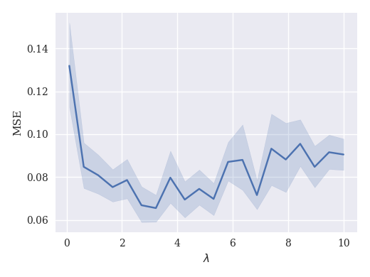
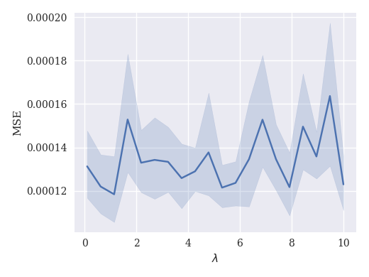


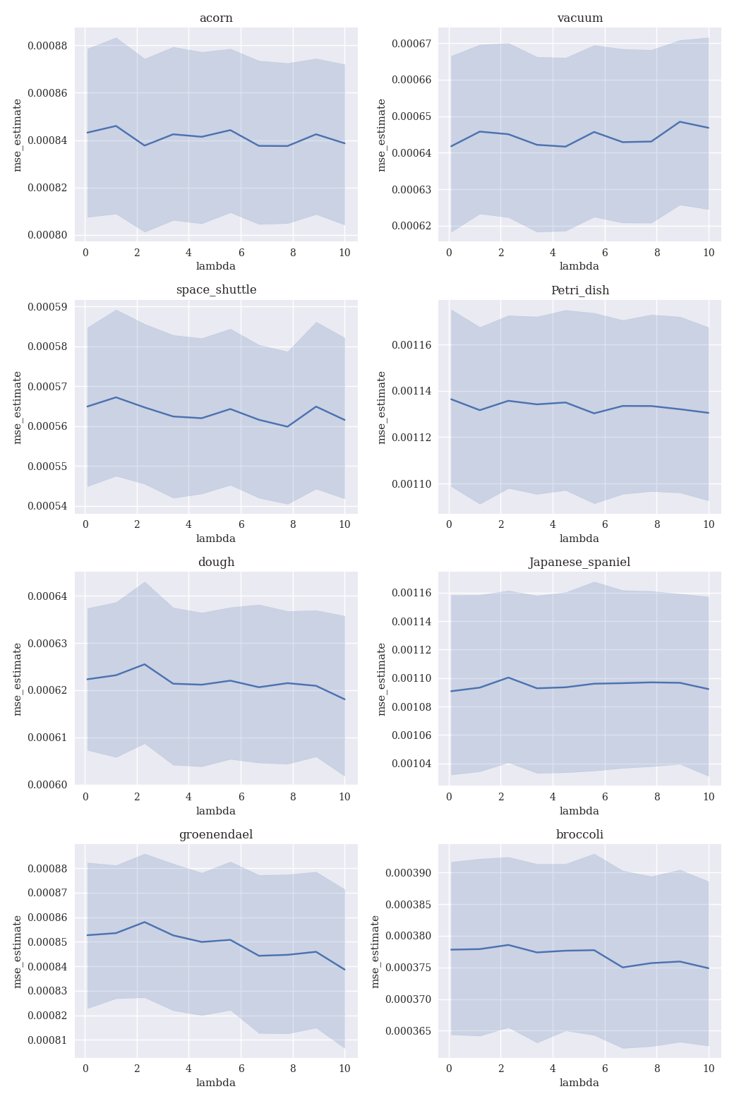
It is also necessary to choose the number of argmax samples for the herding and SBQ algorithms. Recall from Section 3.1 that we approximate the argmax in herding and SBQ, choosing a new permutation sample by selecting a set of uniform random permutations and selecting one to minimise the discrepancy. Figure 16 shows the effect of varying the number of argmax samples on mean squared error for tabular datasets and GBDT models. We find that 5 to 10 samples is too low for optimal performance, but there is little difference between 25 and 50 samples, so choose 25 samples as a compromise for good accuracy and reasonable runtime.


Given the parameters for the Mallows kernel above, we can also compare it to the Spearman and Kendall tau kernels introduced in Section 3 using the herding algorithm. Figure 17 compares the performance of these kernels on tabular data with GBDT models. The Mallows kernel is applied with , and all kernels are using 25 argmax samples. The Spearman kernel is clearly outperformed by both other kernels. The Kendall Tau kernel is effective for 4 out of 6 datasets, but lags behind for make_regression and cal_housing. The Mallows kernel is either the most effective, or within a 95% confidence interval of the most effective kernel for all datasets. For this reason, as well as its universal property, we use the Mallows kernel exclusively in the experiments of Section 5.


