Fluctuations analysis of the spin susceptibility: Néel ordering revisited in dynamical mean field theory

The analytic technique, which we put forward in this paper, can be, in principle, applied to a variety of model systems, which feature fluctuations in different scattering channels. Here, we demonstrate its validity and applicability for the three-dimensional ($3d$) single-band Hubbard model on a simple cubic lattice with nearest-neighbor hopping

where $\hat{c}^{(\dagger)}_{i\sigma}$ annihilates (creates) an electron with spin $\sigma\!=\!\uparrow\!,\!\downarrow$ at the lattice site $\mathbf{R}_{i}$ while $\hat{n}_{i\sigma}\!=\!\hat{c}^{\dagger}_{\sigma}\hat{c}_{i\sigma}$ corresponds to the particle number operator. Moreover, $t_{\text{3d}}$ denotes the amplitude for electrons hopping between nearest-neighbor lattice sites in the $3d$ lattice, $\mu$ is the chemical potential, and $U$ corresponds to the local repulsive Hubbard interaction between the particles. In the following, we use $D\!=\!2\sqrt{6}t_{\text{3d}}\!=\!1$ as unit of energy, which corresponds to twice the second moment of the density of states of the non-interacting system. The average number of particles per lattice site is fixed to $n\!=\!\langle\hat{n}_{\uparrow}\!+\!\hat{n}_{\downarrow}\rangle\!=\!1$.

We apply the DMFT to solve the Hubbard model in Eq. (1). Within this approach, the electronic propagator is dressed with a local self-energy $\Sigma(\nu)$ that depends only on the Matsubara frequencies. The lattice Green’s function is then obtained via Dyson’s equation

where $\epsilon_{\mathbf{k}}\!=\!-t_{\text{3d}}\sum_{<0j>}e^{i\mathbf{k}\mathbf{R}_{j}}$ is the bare dispersion relation and the sum over $j$ runs over the six nearest neighbors of the lattice site at the origin. $\nu\!=\!\frac{\pi}{\beta}(2n\!+\!1)$, $n\in\mathds{Z}$, denotes a fermionic Matsubara frequency with $\beta\!=\!\frac{1}{T}$ being the inverse temperature. Later, we will also consider bosonic Matsubara frequencies $\omega\!=\!\frac{\pi}{\beta}2m$, $m\in\mathds{Z}$.

The local self-energy $\Sigma(\nu)$ is obtained from an auxiliary Anderson impurity model (AIM):

where $\Delta(\nu)$ describes the hybridization between the impurity and the non-interacting bath sites and the local impurity Green’s function $G_{\text{loc}}(\nu)$ is obtained for a given $\Delta(\nu)$ from an impurity solver such as exact diagonalization (ED) or quantum Monte Carlo (QMC). Within DMFT, the hybridization function $\Delta(\nu)$ is determined by the requirement that the local (i.e., momentum-summed) part of the lattice Green’s function is equal to the local Green’s function of the auxiliary AIM:

where $\sum_{\mathbf{k}}$ corresponds to a (normalized) integral over the first Brillouin zone. When a QMC solver is used, $G_{\text{loc}}(\nu)$ can be directly obtained from $\Delta(\nu)$ while for exact diagonalization the hybridization function has to be fitted to a finite number of bath parameters:

where $\varepsilon_{\ell}$ defines the on-site energy of the bath site and $V_{l}$ the hopping amplitude between the bath site and the impurity. Within our ED implementation, these parameters are fitted to a given $\Delta(\nu)$, which is obtained from the self-consistency relation in Eq. (4), for a finite number $N$ of bath sites via a conjugate gradient method.

While the single-particle Green’s function $G(\nu,\mathbf{k})$ provides information about the one-particle spectral properties of the system, two-particle correlation functions are required to describe collective (bosonic) excitations of the electrons. Theoretically, such excitations can be characterized by response functions, the (physical) susceptibilities

where, for the Hubbard model, we consider the charge ($r$=ch) density $\hat{O}_{i}^{r}\!=\!\hat{n}_{i}\!-\!n\!=\!\hat{n}_{i\uparrow}\!+\!\hat{n}_{i\downarrow}\!-\!n$, the spin ($r$=sp) density $\hat{O}_{i}^{r}\!=\!\hat{S}^{z}_{i}\!=\!\hat{n}_{i\uparrow}\!-\!\hat{n}_{i\downarrow}$ and the particle-particle ($r$=pp) pair density $\hat{O}_{i}^{r}\!=\!\hat{c}^{\dagger}_{i\uparrow}\hat{c}^{\dagger}_{i\downarrow}\!+\!\hat{c}_{i\downarrow}\hat{c}_{i\uparrow}$ at the lattice site $\mathbf{R}_{i}$. Completely analogous definitions hold for the AIM where the spatial index $i$ as well as the Fourier transform $\sum_{i}e^{-i\mathbf{q}\cdot\mathbf{R}_{i}}$ have to be omitted.

A (second-order) phase transition to a spatially ordered state in one of the three fluctuation channels is signaled by a divergence of the corresponding susceptibility at $\omega\!=\!0$ and $\mathbf{q}\!=\!\mathbf{q}_{0}$ where $\mathbf{q}_{0}$ defines the spatial structure of the order. In the half filled Hubbard model, the leading instability is found in the spin channel at $\mathbf{q}_{0}\!=\!(\pi,\pi,\pi)\!\equiv\!\boldsymbol{\Pi}$, which corresponds to antiferromagnetic spin fluctuations, i.e.,

At the Néel temperature $T\!=\!T_{N}$, at which the transition to the antiferromagnetically ordered state occurs, this response function diverges, i.e.,

This criterion has been used for the determination of $T_{N}$ in this paper.

The physical susceptibilities defined in Eq. (6) can be obtained from more general objects, the generalized susceptibilities¹¹ 1 Here, we have already considered the case of DMFT where the generalized lattice susceptibility depends only a single momentum $\mathbf{q}$. In the most general case, this object exhibits also a dependence on two additional momenta $\mathbf{k}$ and $\mathbf{k}^{\prime}$. $\chi_{r,\mathbf{q}}^{\nu\nu^{\prime}\omega}$, by summing the latter over the fermionic Matsubara frequencies $\nu$ and $\nu^{\prime}$:

The generalized susceptibilities are calculated via a Bethe-Salpeter equation (BSE) from an irreducible vertex function $\Gamma_{r}^{\nu\nu^{\prime}\omega}$, which is local but frequency dependent within DMFTGeorges et al. 1996. In the channel of interest, i.e., the spin channel, the relevant BSE reads

Here, $\chi_{0,\mathbf{q}}^{\nu\nu^{\prime}\omega}\!=\!-\beta\sum_{\mathbf{k}}G(\nu,\mathbf{k})G(\nu\!+\!\omega,\mathbf{k}\!+\!\mathbf{q})\delta_{\nu\nu^{\prime}}$ is the bare susceptibility (“bubble”) of DMFT. The local irreducible vertex in the spin channel $\Gamma_{\text{sp}}^{\nu\nu^{\prime}\omega}$, on the other hand, can be calculated via a purely local Bethe-Salpeter equation [analogous to Eq. (10)] from the corresponding local generalized susceptibility $\chi_{\text{sp}}^{\nu\nu^{\prime}\omega}$, which, in turn, is obtained directly from the AIM related to the DMFT solution of the Hubbard model in Eq. (1) by means of the impurity solver (see, e.g., Ref. Toschi et al. 2007).

The main goal of our paper is to understand how the frequency-dependent vertex $\Gamma_{\text{sp}}^{\nu\nu^{\prime}\omega}$ affects the generalized and the physical susceptiblities in Eqs. (10) and (9), respectively. More specifically, we want to understand how the frequency dependence of $\Gamma_{\text{sp}}^{\nu\nu^{\prime}\omega}$ changes the related $T_{N}$ with respect to a simple random phase like calculation where the irreducible vertex in Eq. (10) is replaced by the bare interaction $U$. Moreover, we aim at unraveling which (Feynman diagrammatic) contributions to $\Gamma_{\text{sp}}^{\nu\nu^{\prime}\omega}$ lead to specific modifications of the critical temperature, resulting in an increase or a reduction of $T_{N}$. To make such an analysis meaningful, it would be of course highly desirable to identify the parts of the vertex to which a transparent physical meaning can be assigned.

In the last decade, considerable progress has been made in the understanding of the frequency structure of two-particle vertex functionsKuneŝ 2011; Rohringer et al. 2012; Hafermann 2014; Rohringer et al. 2018; Krien et al. 2019; Stepanov et al. 2019; Chalupa et al. 2018; Springer et al. 2020; Wentzell et al. 2020; Chalupa et al. 2021. In particular, it has been demonstrated that some of the main features of these correlation functions (which are also responsible for their high-frequency behavior) correspond to physical observables, which are even experimentally accessible, i.e., the physical susceptibilities, which are defined in Eq. (9). Taking into account only these contributions gives rise to the following approximation for the irreducible vertex, which has been discussed in Ref. Tagliavini et al. 2018 (see also the supplemental material of Ref. Gunnarsson et al. 2015 as well as Refs. Krien et al. 2019 and Stepanov et al. 2019):

where $\chi^{\text{loc}}_{\text{sp}}(\omega)$, $\chi^{\text{loc}}_{\text{ch}}(\omega)$, and $\chi^{\text{loc}}_{\text{pp}}(\omega)$ denote the local spin, charge, and particle-particle (up-down) susceptibility of DMFT, which can be obtained directly from the related AIM. Let us point out that no susceptibility, which depends only on the bosonic Matsubara frequency $\omega$ appears in Eq.(II.3) since such contribution corresponds to reducible vertex diagrams, which are present in the fullGunnarsson et al. 2015; Tagliavini et al. 2018 but not in the irreducible vertex. We also want to remark that the concrete form of Eq. (II.3) holds for frequency and time independent interactions in the SU(2) symmetric case.

The approximate form of $\Gamma_{\text{sp}}^{\nu\nu^{\prime}\omega}$ in Eq. (II.3) provides a starting point to investigate the impact of the different local fluctuations of DMFT in the charge, spin, and particle-particle channels on the antiferromagnetic susceptibility and, consequently, on the transition temperature $T_{N}$ to the antiferromagnetically ordered state. This will be achieved by “switching” on and off the various contributions to the local irreducible vertex. To this end we define

where for convenience we have introduced the effective screened interactions $W_{r}^{\omega}\!=\!U^{2}\chi_{r}^{\text{loc}}(\omega)$ and the binary weights $w_{r}=\{0,1\}$ that switch on or off the contributions of the different local fluctuations. Note that we have restricted Eq. (12) already to the relevant case $\omega\!=\!0$. The above procedure gives rise to $8$ different approximations for $\Gamma_{\text{sp}}^{\nu\nu^{\prime}(\omega=0)}$ where this correlation function includes the local fluctuations of DMFT in $0$, $1$, $2$, or all $3$ fluctuation channels. The corresponding numerical results for the $8$ $T_{N}$ curves for all possible combinations of the three binary weights $w_{r}$ are discussed in the first part of Sec. III.

An approximation, which is similar to Eq. (II.3), has been put forward in Ref. Tahvildar-Zadeh et al. 1997 where only the second-order contribution (bubble terms) to the local susceptibilities has been taken into account. While we will start from the perturbative expressions of $\chi_{r}^{\text{loc}}(\omega)$ we will also consider the fully dressed version of these correlation functions, which contain all local vertex corrections.

Nevertheless, it is far from obvious what can be expected from such approximations for $\Gamma_{\text{sp}}^{\nu\nu^{\prime}(\omega=0)}$ beyond the weak-to-intermediate coupling regime. In fact, in this region of the phase diagram the contributions from the fermion-boson triangular verticesHarkov et al. 2021 or the fully irreducible vertices might become non-negligible. To improve our understanding of the AF phase transition also for stronger values of $U$, we propose, as a second step, an inverse or complementary fluctuation analysis of the AF susceptibility where we start from the exact irreducible vertex $\Gamma_{\text{sp}}^{\nu\nu^{\prime}(\omega=0)}$ of DMFT and subtract the contributions originating from the local susceptibilities in the charge, spin, and particle-particle channels (note that the spin contribution is negative)

In this way, we keep all nonperturbative low-frequency contributions of the irreducible vertex but we are still able to “switch” on and off the high-frequency local fluctuations contained in these correlation functions. The results for this complementary way of the fluctuation analysis will be presented in the second part of Sec. III.

One of the simplest approaches to calculate $\chi_{\text{sp}}(\omega,\mathbf{q})$ and $T_{N}$ for $\frac{U}{t}\ll 1$ is the RPA, a static mean field theory. Within the formal framework discussed in the previous sections, this corresponds to $\Sigma(\nu)\!=\!0$ and $\Gamma_{\text{sp}}^{\nu\nu^{\prime}\omega}\!=\!-U$. In three dimensions, RPA gives rise to a $T_{N}$, which increases exponentially with $U$ as $T_{N}^{\text{RPA}}\!\propto\!e^{-\frac{1}{UD(0)}}$ (see dashed pink curve in Fig. 1) where $D(0)$ is the noninteracting density of states at the Fermi level. A first attempt to understand how local DMFT correlations modify this picture was made in Ref. Tahvildar-Zadeh et al. 1997 (see also Refs. Schauerte and van Dongen 2002 and Keller et al. 2001): There the authors approximated $\Gamma_{\text{sp}}^{\nu\nu^{\prime}\omega}$ by a simple second-order diagram, which gave rise to a reduction of $T_{N}$ by roughly a factor of $3$ (solid brown curve) matching rather well the exact DMFT value (filled violet squares) at small $U$. Hence, the authors concluded that the introduction of local DMFT vertex corrections in $\Gamma_{\text{sp}}^{\nu\nu^{\prime}\omega}$ leads to a suppression of $T_{N}$.

Let us now view this second-order approximation from a more general perspective in the framework of Eqs. (II.3) and (12): At second order in $U$, the local spin and charge susceptibilities are equivalent [$\chi_{\text{sp}}^{(2),\text{loc}}(\omega)\!=\!\chi_{\text{ch}}^{(2),\text{loc}}(\omega)\!=\!-\frac{1}{\beta}\sum_{\nu}G_{\text{loc}}(\nu)G_{\text{loc}}(\nu\!+\!\omega)$] and, hence, cancel in the approximate expression for $\Gamma_{\text{sp}}^{\nu\nu^{\prime}\omega}$. Thus, only the particle-particle contribution remains, which—due to the above mentioned cancellation—corresponds to either $w_{\text{ch}}\!=\!w_{\text{sp}}\!=\!0$ or $w_{\text{ch}}\!=\!w_{\text{sp}}\!=\!1$ and $w_{\text{pp}}\!=\!1$ in Eq. (12).

We now consider other combinations of the binary weights $w_{r}$ to gain more insight into the impact of the different local fluctuations on $T_{N}$, where we again take into account only the second-order contributions for $\chi_{r}^{\text{loc}}(\omega)$. In Fig. 2 we can clearly see, that for all combinations of $w_{r}$ where $w_{\text{sp}}\!=\!0$ and at least one of the two other weights $w_{\text{ch}}$ and/or $w_{\text{pp}}$ equals $1$ (dashed brown and cyan and solid black lines) the corresponding $T_{N}$ is lower than the RPA value (thick pink line). Hence, local charge and particle-particle fluctuations lead to a screening of the bare interaction $U$ in $\Gamma_{\text{sp}}^{\nu\nu^{\prime}\omega}$. Interestingly, the reduction of $T_{N}$ with respect to RPA due to local particle-particle fluctuations (dashed brown line) is stronger than due to charge fluctuations (dashed cyan line) although both types of fluctuations are equivalent at half filling, i.e., $\chi_{\text{ch}}^{\text{loc}}(\omega)\!\equiv\!\chi_{\text{pp}}^{\text{loc}}(\omega)$. This can be easily understood from Eqs. (II.3) and (12) where the local particle-particle susceptibility enters the vertex $\Gamma_{\text{sp}}^{\nu\nu^{\prime}\omega}$ with a factor of $2$ compared to the charge susceptibility.

On the contrary, the combination $w_{\text{sp}}\!=\!1$ and $w_{\text{ch}}\!=\!w_{\text{pp}}\!=\!0$ (solid blue line) leads to a larger $T_{N}$ with respect to RPA. Hence, local spin fluctuations lead to a “negative” screening of $U$ in $\Gamma_{\text{sp}}^{\nu\nu^{\prime}\omega}$, which is consistent with the negative sign of $\chi_{\text{sp}}^{\text{loc}}(\omega)$ in Eqs. (II.3) and (12). Let us stress that no further curves for $T_{N}$ can be obtained from the three missing combinations of $w_{r}$ within second-order perturbation theory due to the equivalence of all three local susceptibilities in this approximation²² 2 Due to the equivalence of all three local susceptibilities the combination $w_{\text{sp}}\!=\!w_{\text{ch}}\!=\!w_{\text{pp}}\!=\!1$ is equivalent to $w_{\text{sp}}\!=\!w_{\text{ch}}\!=\!0$, $w_{\text{pp}}\!=\!1$, the combination $w_{\text{sp}}\!=\!w_{\text{ch}}\!=\!1$, $w_{\text{pp}}\!=\!0$ is equivalent to $w_{\text{sp}}\!=\!w_{\text{ch}}\!=\!=w_{\text{pp}}\!=\!0$ and the combination $w_{\text{sp}}\!=\!w_{\text{pp}}\!=\!0$, $w_{\text{ch}}\!=\!1$ is equivalent to $w_{\text{sp}}\!=\!w_{\text{pp}}\!=\!1$, $w_{\text{ch}}\!=\!0$..

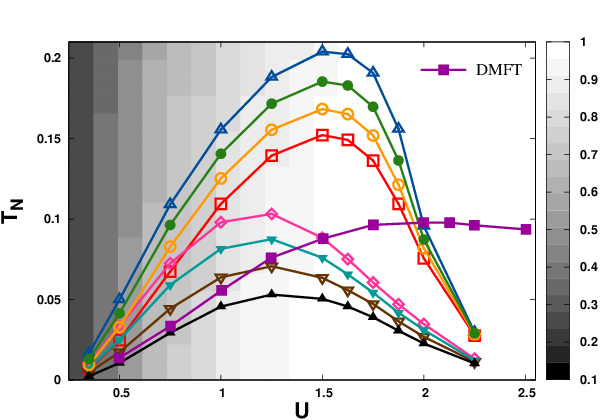
Figure 4 shows the fluctuation analysis of $T_{N}$ in a larger $U$ region where the same colors and symbols for the different combinations of the $w_{r}$’s have been used as in the weak-coupling analysis in Fig. 2. For $U\!\geq\!1$, we observe a clear hierarchy of the curves for $T_{N}$ calculated with the different approximations of $\Gamma_{\text{sp}}^{\nu\nu^{\prime}\omega}$: All results for the transition temperature obtained by setting $w_{\text{sp}}\!=\!0$ (filled cyan lower triangles, empty brown lower triangles, filled black upper triangles) lie below the pink curve (empty diamonds), which represents the result for $T_{N}$ without vertex corrections [$\Gamma_{\text{sp}}^{\nu\nu^{\prime}\omega}\!=\!-U$, $w_{r}\!=\!0$ for all channels $r$ in Eq. (12)]. This is consistent with the weak-coupling result that local charge and particle-particle fluctuations in $\Gamma_{\text{sp}}^{\nu\nu^{\prime}\omega}$ lead to a screening of the bare interaction $-U$ in this vertex function and, hence, reduce the transition temperature with respect to to $\Gamma_{\text{sp}}^{\nu\nu^{\prime}\omega}\!=\!-U$. This reduction is obviously largest when both (i.e., charge and particle-particle) screening channels contribute to $\Gamma_{\text{sp}}^{\nu\nu^{\prime}\omega}$ ($w_{\text{ch}}\!=\!w_{\text{pp}}\!=\!1$, filled black upper triangles in Fig. 4). Although at half filling local charge and particle-particle fluctuations are equivalent, the latter (empty brown lower triangles) suppress $T_{N}$ stronger than the inclusion of charge fluctuations (filled cyan lower triangles). As already pointed out in the weak-coupling analysis, this can be ascribed to the different prefactors with which $\chi_{\text{pp}}^{\text{loc}}$ and $\chi_{\text{ch}}^{\text{loc}}$ enter Eqs. (II.3) and (12).

Conversely, we find the opposite effect when spin fluctuations are included: For $U\!\geq\!1$, all curves for $T_{N}$ in Fig. 4 where $w_{\text{sp}}\!=\!1$ (empty blue upper triangles, filled green circles, empty orange circles, empty red squares) lie above the pink diamonds for which all vertex corrections for $\Gamma_{\text{sp}}^{\nu\nu^{\prime}\omega}$ are neglected. Hence, local spin fluctuations provide a “negative” screening, which enhances the bare interaction and, consequently, the antiferromagnetic susceptibility and $T_{N}$ with respect to the calculation with $\Gamma_{\text{sp}}^{\nu\nu^{\prime}\omega}\!=\!-U$. The situation where only local spin fluctuations are considered (i.e., $w_{\text{sp}}\!=\!1$ and $w_{\text{ch}}\!=\!w_{\text{pp}}\!=\!0$, empty blue upper triangles) obviously gives rise to the largest $T_{N}$ while the inclusion of one or both of the two other channels leads to a smaller value of $T_{N}$. However, for $U\!\geq\!1$, the screening provided by the local charge and particle-particle fluctuations is always smaller than the enhancement of $\Gamma_{\text{sp}}^{\nu\nu^{\prime}\omega}$ due to local spin fluctuations.

The above considerations are obviously an effect of the strong enhancement of local spin fluctuations with respect to local charge and particle-particle fluctuations upon increasing $U$ within DMFT. Hence, it is interesting to analyze the relative difference between $\chi^{\text{loc}}_{\text{sp}}$ and $\chi^{\text{loc}}_{\text{ch}}$ (which is equivalent to $\chi^{\text{loc}}_{\text{pp}}$ at half filling) as a function of $U$. This is shown in Fig. 4 by means of a gray-scale intensity map that encodes the relative deviation between the static ($\omega\!=\!0$) charge and spin fluctuations defined as $\frac{\chi_{s}(\omega=0)-\chi_{c}(\omega=0)}{\chi_{s}(\omega=0)+\chi_{c}(\omega=0)}=-\frac{\chi_{\uparrow\downarrow}(\omega=0)}{\chi_{\uparrow\uparrow}(\omega=0)}$. At $U\!=\!0$, this ratio vanishes exactly while for $U\!\rightarrow\!\infty$ it approaches unity. Hence, when the relative deviation increases (brighter gray shades in Fig. 4), spin fluctuations in $\Gamma_{\text{sp}}^{\nu\nu^{\prime}\omega}$ gradually become dominant. Consistently with the discussion above, such a dominance of spin fluctuations is observed already in the weak-to-intermediate coupling regime at $U\!\geq\!1$ where the relative deviation is about 80% (although this is well below the Mott local moment regime, which sets in at $U\!\sim\!2.3$).

Let us briefly comment on the general structure of $T_{N}$ as a function of $U$ in Fig. 4. We observe a qualitatively similar behavior as for the exact DMFT phase transition (filled violet squares): At small values of $U$, $T_{N}$ increases, then reaches a maximum at intermediate coupling and decreases at large values of $U$. However, on a quantitative level it is quite clear that Eqs. (II.3) and (12) do not provide a good approximation for $\Gamma_{\text{sp}}^{\nu\nu^{\prime}\omega}$ to calculate $T_{N}$. In fact, the maxima of $T_{N}$ for the approximate calculations are shifted with respect to the DMFT result and, moreover, the vertex in Eq.(12) fails completely to recover the strong-coupling limit where $T_{N}\propto t^{2}/U$. In this regime, the bubble goes to zero too rapidly and even in the case with $w_{s}\!=\!1$ (and $w_{\text{ch}}^{\text{loc}}\!=\!w_{\text{pp}}^{\text{loc}}\!=\!0)$, the formation of local moments encoded in $\chi_{s}(\omega)$ it is not sufficient to balance the loss of coherence occurring in the bubble via the insertion of the local self-energy in the Green’s function.

This indicates that beyond weak coupling contributions to the irreducible vertex $\Gamma_{\text{sp}}^{\nu\nu^{\prime}\omega}$ become important, which are not considered in Eqs. (II.3) and (12). Within the dual fermion approach, a good quantitative agreement has been achieved in the framework of the single-boson exchange formalismHarkov et al. 2021, which includes additional contributions in the expansion, in particular the triangular vertices, which account for the coupling between the electrons and the collective modes. In the latter situation the approximations have been performed in a dual space to the full (instead of the irreducible) local vertex of DMFT. The inclusion of triangular vertices also in the approximation for $\Gamma_{\text{sp}}^{\nu\nu^{\prime}\omega}$ in Eq. (II.3) would be definitely interesting and can potentially improve our results. However, in this paper we follow the alternative route outlined in Sec. II.4 leaving the question of the triangular vertices for future research work.

Figure 5 suggests that the three curves, where local charge and/or particle-particle fluctuations are subtracted (blue upper empty triangles, green filled circles, orange empty circles), approach the DMFT transition line in the limit $U\!\rightarrow\!\infty$. This is reasonable since local charge and particle-particle fluctuations are exponentially suppressed in the large coupling limit. To verify this intuitive argument, we consider the following useful approximation for the calculation of $T_{N}$ at large $U$, which recovers the expected power-law behavior of the critical temperature.

Solving Eq. (10) for the (inverse of the) generalized spin susceptibility $\chi_{\mathbf{\text{sp},q}}^{\nu\nu^{\prime}\omega}$ yields

where we chose a matrix notation in the fermionic Matsubara frequencies, i.e., $\bar{\bar{\chi}}(\omega,\mathbf{q})\!=\!\left[\bar{\bar{\chi}}(\omega,\mathbf{q})\right]_{\nu\nu^{\prime}}\!\equiv\!\chi^{\nu\nu^{\prime}\omega}_{\mathbf{q}}$ and “^-1” denotes the inversion of this (infinite) matrix. The local irreducible vertex $\Gamma_{\text{sp}}^{\nu\nu^{\prime}\omega}$, in turn, can be obtained from a purely local version of the BS Eq. (10), which reads

where $\bar{\bar{\chi}}^{-1}_{\text{sp}}(\omega)$ is the local generalized spin susceptibility of the auxiliary AIM and $\bar{\bar{\chi}}_{0}(\omega)=\chi_{0}^{\nu\nu^{\prime}\omega}\!=\!-\beta G(\nu)G(\nu+\omega)\delta_{\nu\nu^{\prime}}$ is the local bubble. Combining Eqs. (14) and (15) then yields

The AF susceptibility corresponds to $\omega\!=\!0$ and $\mathbf{q}\!=\!\boldsymbol{\Pi}$ in this equation. Due to the DMFT self-consistency condition, the nonlocal bubble term reduces to $\bar{\bar{\chi}}_{0}(\omega\!=\!0,\mathbf{q}\!=\!\boldsymbol{\Pi})=-\beta\mathbbm{1}\,D(\zeta_{\nu})/\zeta_{\nu}$, where we have introduced the Hilbert transform $D(\zeta)=\int_{-\infty}^{+\infty}d\epsilon g(\epsilon)[\zeta-\epsilon]^{-1}$ of the noninteracting density of states $g(\epsilon)$, with $\zeta_{\nu}=i\nu+\mu-\Sigma(\nu)$ ($\mathbbm{1}\!=\!\delta_{\nu\nu^{\prime}}$ is the unit matrix in the $\nu$-$\nu^{\prime}$ space). The local bubble, on the other hand, can be expressed in terms of the Hilbert transform as $\bar{\bar{\chi}}_{0}(\omega=0)=-\beta\mathbbm{1}\,D^{2}(\zeta_{\nu})$. In the specific case of a semi-circular density of states $g(\epsilon)=\frac{1}{2\pi t^{2}}\sqrt{\epsilon^{2}-4t^{2}}$ (Bethe lattice), the contribution arising from the bubble terms simplifies considerably and Eq.(16) reduces to

We recall that a very similar formula is found for the homogeneous case q = 0 Georges et al. 1996; Del Re and Capone 2018; Reitner et al. 2020 where where $-t^{2}$ is replaced with $+t^{2}$ . To make contact to the $3d$ lattice model considered before, we choose $t$ in such a way that twice the second moment of the density of states $g(\epsilon)$ of the Bethe lattice is normalized to $D\!=\!1$ (as for the $3d$ cubic lattice). Here, this corresponds to $D\!=\!2t\!=\!1$, i.e., $t\!=\!\sqrt{6}t_{\text{3d}}$. With this choice both lattice types will lead to quantitatively same results for the local correlation functions of DMFT since the DMFT self-consistency is mainly controlled by the second moment of the non-interacting density of statesBulla and Potthoff 2000. For the nonlocal spin susceptibility and the related $T_{N}$ this also holds at strong coupling where these quantities are mainly governed by the local DMFT self-energy and irreducible vertex functions. This can be seen in Fig. 6 where the dashed blue line, which corresponds to $T_{N}$ as obtained from the expression in Eq. (17) for the Bethe lattice (but with the local correlation functions obtained from a DMFT calculation for the simple cubic lattice), agrees very well with the exact DMFT calculation for the simple cubic lattice (filled violet squares). On the other hand, at weaker coupling $T_{N}$ is mainly determined by the noninteracting density of states ($T_{N}^{\text{RPA}}\!\propto\!e^{-\frac{1}{UD(0)}}$) at zero energy, which is in general different for the Bethe and the simple cubic lattice when their second moments are fixed to the same value. This can explain the different results for $T_{N}$ from DMFT and the Bethe lattice treatment in this parameter regime.

Starting from Eq.(17), an obvious approximation for the strong coupling limit consists in replacing $\bar{\bar{\chi}}_{\text{sp}}(0)$ by the corresponding generalized susceptibility calculated in the atomic limit $\bar{\bar{\chi}}^{\text{AL}}_{\text{sp}}(0)$. The inverse of $\bar{\bar{\chi}}_{\text{sp}}^{\text{AL}}(0)$, which is required in Eq. (17), has been calculated analytically (at half filling) in Ref. Thunström et al. 2018. The same methods, which have been used for the inversion of the $\bar{\bar{\chi}}_{\text{sp}}^{\text{AL}}(\omega)$ in this paper, can be applied to invert $\bar{\bar{\chi}}_{\text{sp}}^{-1}(0,\boldsymbol{\Pi})$ in Eq. (17). The transition temperature $T_{N}$ is then determined by the condition that the matrix $\bar{\bar{\chi}}_{\text{sp}}^{-1}(0,\boldsymbol{\Pi})$ is singular, corresponding to a divergence of $\bar{\bar{\chi}}_{\text{sp}}(0,\boldsymbol{\Pi})$. From this condition we obtain the following expression of $T_{N}$ in terms of $T$, $U$, and $t$ (for details see Appendix B):

Considering only the leading order in $t/U$, this equation obviously reproduces the large $U$ behavior of $T_{N}$ given by $T_{N}\sim t^{2}/U$.

This is also illustrated in Fig. 6, where we show that the Néel temperature, calculated within the AL approximation (filled orange circles), coincides with the exact DMFT result (filled violet squares) for $U\gtrsim 2.5$ and reproduces the correct large coupling limit $T_{N}\sim t^{2}/U$ (green line).

To perform the fluctuation analysis of $T_{N}$ for $U\rightarrow\infty$, we consider the susceptibilities in the atomic limit

We can see that $\chi_{\text{ch}}^{\text{loc}}$ and $\chi_{\text{pp}}^{\text{loc}}$ vanish exponentially with $U$. Since we have neglected such terms in Eq. (18), there is no contribution from these fluctuations to $T_{N}$ in the large coupling limit and, hence, all lines of the complementary fluctuation analysis in Fig. 5, where $\chi_{\text{sp}}^{\text{loc}}$ has not been subtracted, should collapse on the DMFT curve for $U\rightarrow\infty$. It is, however, interesting that even for the largest $U$ value, where the exponential suppression of local charge and particle-particle susceptibilities is already rather strong, the difference between the curves is still sizable. Indeed, if we would have used the corresponding local charge and particle-particle susceptibilities of the AL (instead of the exact DMFT ones) the curves would have already collapsed onto the DMFT line at $U~\sim 3.0$. This indicates that local DMFT charge and particle-particle fluctuations cannot completely be neglected in this parameter regime. To quantify this statement we have calculated the ratio $\chi_{\text{ch}}^{\text{loc}}(\omega\!=\!0)/\chi_{\text{sp}}^{\text{loc}}(\omega\!=\!0)$ in both the DMFT and the AL. At the largest value of the interaction ($U\!=\!4$) and at a temperature close to the phase transition ($\beta\!=\!16$), this ratio is given by $5.5\times 10^{-4}$ within DMFT. This is indeed one order of magnitude smaller than the absolute difference between $T_{N}$ of DMFT (red filled squares in Fig. 5) and the transition temperature obtained by removing charge fluctuations (orange empty circles in Fig. 5). The corresponding ratio calculated using the same set of parameters but in the AL from Eqs. (19) yields a value of $1.3\times 10^{-14}$, which is about 10 orders of magnitudes smaller than the DMFT result.

It is worth to notice that it is highly important how the AL approximation is performed in our calculations. In fact, we did not replace the irreducible vertex $\Gamma_{\text{sp}}^{\nu\nu^{\prime}\omega}$ with the one of the atomic limit, which would not reproduce the correct behavior of $T_{N}$ at strong coupling. This is similar to the two options how $T_{N}$ of DMFT for large $U$ can be calculated within the dual fermion formalism as it has been discussed in Ref. Krien 2019. There, two types of approximations have been performed for the full (instead of the irreducible) vertex. Again only one of these approximations produces the correct large $U$ behavior of $T_{N}$. How this is linked to the approximations presented in this paper is an interesting open question for future research work.

References

- Mott (1968) N. F. Mott, Rev. Mod. Phys. 40, 677 (1968).
- Bednorz and Müller (1986) J. G. Bednorz and K. A. Müller, Zeitschrift fur Physik B Condensed Matter 64, 189 (1986).
- Néel, Louis (1936) Néel, Louis, Ann. Phys. 11, 232 (1936).
- Kohn and Sham (1965) W. Kohn and L. J. Sham, Phys. Rev. 140, A1133 (1965).
- Georges et al. (1996) A. Georges, G. Kotliar, W. Krauth, and M. J. Rozenberg, Rev. Mod. Phys. 68, 13 (1996).
- Hubbard (1963) J. Hubbard, Proceedings of the Royal Society of London. Series A, Mathematical and Physical Sciences 276, 238 (1963).
- Astretsov et al. (2020) G. V. Astretsov, G. Rohringer, and A. N. Rubtsov, Phys. Rev. B 101, 075109 (2020).
- Zheng and Chan (2016) B.-X. Zheng and G. K.-L. Chan, Phys. Rev. B 93, 035126 (2016).
- Qin et al. (2020) M. Qin, C.-M. Chung, H. Shi, E. Vitali, C. Hubig, U. Schollwöck, S. R. White, and S. Zhang (Simons Collaboration on the Many-Electron Problem), Phys. Rev. X 10, 031016 (2020).
- Schrieffer and Wolff (1966) J. R. Schrieffer and P. A. Wolff, Phys. Rev. 149, 491 (1966).
- Tahvildar-Zadeh et al. (1997) A. N. Tahvildar-Zadeh, J. K. Freericks, and M. Jarrell, Phys. Rev. B 55, 942 (1997).
- Rohringer et al. (2012) G. Rohringer, A. Valli, and A. Toschi, Phys. Rev. B 86, 125114 (2012).
- Rohringer (2013) G. Rohringer, New routes towards a theoretical treatment of nonlocal electronic correlations, Ph.D. thesis, Vienna University of Technology (2013).
- Gunnarsson et al. (2015) O. Gunnarsson, T. Schäfer, J. P. F. LeBlanc, E. Gull, J. Merino, G. Sangiovanni, G. Rohringer, and A. Toschi, Phys. Rev. Lett. 114, 236402 (2015).
- Tagliavini et al. (2018) A. Tagliavini, S. Hummel, N. Wentzell, S. Andergassen, A. Toschi, and G. Rohringer, Phys. Rev. B 97, 235140 (2018).
- Wentzell et al. (2020) N. Wentzell, G. Li, A. Tagliavini, C. Taranto, G. Rohringer, K. Held, A. Toschi, and S. Andergassen, Phys. Rev. B 102, 085106 (2020).
- Krien et al. (2019) F. Krien, A. Valli, and M. Capone, Phys. Rev. B 100, 155149 (2019).
- Stepanov et al. (2019) E. A. Stepanov, V. Harkov, and A. I. Lichtenstein, Phys. Rev. B 100, 205115 (2019).
- Krien et al. (2020) F. Krien, A. I. Lichtenstein, and G. Rohringer, Phys. Rev. B 102, 235133 (2020).
- Wu et al. (2017) W. Wu, M. Ferrero, A. Georges, and E. Kozik, Phys. Rev. B 96, 041105 (2017).
- Schäfer and Toschi (2021) T. Schäfer and A. Toschi, Journal of Physics: Condensed Matter 33, 214001 (2021).
- Gunnarsson et al. (2017) O. Gunnarsson, G. Rohringer, T. Schäfer, G. Sangiovanni, and A. Toschi, Phys. Rev. Lett. 119, 056402 (2017).
- Gunnarsson et al. (2018) O. Gunnarsson, J. Merino, T. Schäfer, G. Sangiovanni, G. Rohringer, and A. Toschi, Phys. Rev. B 97, 125134 (2018).
- Rohringer (2020) G. Rohringer, Journal of Electron Spectroscopy and Related Phenomena 241, 146804 (2020), Sources, Interaction with Matter, Detection and Analysis of Low Energy Electrons (SIMDALEE2).
- (25) Here, we have already considered the case of DMFT where the generalized lattice susceptibility depends only a single momentum . In the most general case, this object exhibits also a dependence on two additional momenta and .
- Toschi et al. (2007) A. Toschi, A. A. Katanin, and K. Held, Phys. Rev. B 75, 045118 (2007).
- Kuneŝ (2011) J. Kuneŝ, Phys. Rev. B 83, 085102 (2011).
- Hafermann (2014) H. Hafermann, Phys. Rev. B 89, 235128 (2014).
- Rohringer et al. (2018) G. Rohringer, H. Hafermann, A. Toschi, A. A. Katanin, A. E. Antipov, M. I. Katsnelson, A. I. Lichtenstein, A. N. Rubtsov, and K. Held, Rev. Mod. Phys. 90, 025003 (2018).
- Chalupa et al. (2018) P. Chalupa, P. Gunacker, T. Schäfer, K. Held, and A. Toschi, Phys. Rev. B 97, 245136 (2018).
- Springer et al. (2020) D. Springer, P. Chalupa, S. Ciuchi, G. Sangiovanni, and A. Toschi, Phys. Rev. B 101, 155148 (2020).
- Chalupa et al. (2021) P. Chalupa, T. Schäfer, M. Reitner, D. Springer, S. Andergassen, and A. Toschi, Phys. Rev. Lett. 126, 056403 (2021).
- Harkov et al. (2021) V. Harkov, A. I. Lichtenstein, and F. Krien, Phys. Rev. B 104, 125141 (2021).
- Schauerte and van Dongen (2002) T. Schauerte and P. G. J. van Dongen, Phys. Rev. B 65, 081105 (2002).
- Keller et al. (2001) M. Keller, W. Metzner, and U. Schollwöck, Phys. Rev. Lett. 86, 4612 (2001).
- (36) Due to the equivalence of all three local susceptibilities the combination is equivalent to , , the combination , is equivalent to and the combination , is equivalent to , .
- Del Re and Capone (2018) L. Del Re and M. Capone, Phys. Rev. A 98, 063628 (2018).
- Reitner et al. (2020) M. Reitner, P. Chalupa, L. Del Re, D. Springer, S. Ciuchi, G. Sangiovanni, and A. Toschi, Phys. Rev. Lett. 125, 196403 (2020).
- Bulla and Potthoff (2000) R. Bulla and M. Potthoff, The European Physical Journal B - Condensed Matter and Complex Systems 13, 257 (2000).
- Thunström et al. (2018) P. Thunström, O. Gunnarsson, S. Ciuchi, and G. Rohringer, Phys. Rev. B 98, 235107 (2018).
- Krien (2019) F. Krien, Phys. Rev. B 99, 235106 (2019).
- Del Re et al. (2019) L. Del Re, M. Capone, and A. Toschi, Phys. Rev. B 99, 045137 (2019).
- Rubtsov et al. (2009) A. N. Rubtsov, M. I. Katsnelson, A. I. Lichtenstein, and A. Georges, Phys. Rev. B 79, 045133 (2009).
- Rohringer et al. (2011) G. Rohringer, A. Toschi, A. Katanin, and K. Held, Phys. Rev. Lett. 107, 256402 (2011).
- Rubtsov et al. (2012) A. Rubtsov, M. Katsnelson, and A. Lichtenstein, Annals of Physics 327, 1320 (2012).
- Rohringer et al. (2013) G. Rohringer, A. Toschi, H. Hafermann, K. Held, V. I. Anisimov, and A. A. Katanin, Phys. Rev. B 88, 115112 (2013).
- Rohringer and Toschi (2016) G. Rohringer and A. Toschi, Phys. Rev. B 94, 125144 (2016).
- Ayral and Parcollet (2016a) T. Ayral and O. Parcollet, Phys. Rev. B 94, 075159 (2016a).
- Ayral and Parcollet (2016b) T. Ayral and O. Parcollet, Phys. Rev. B 93, 235124 (2016b).
- Del Re and Toschi (2021) L. Del Re and A. Toschi, Phys. Rev. B 104, 085120 (2021).
- Kitatani et al. (2019) M. Kitatani, T. Schäfer, H. Aoki, and K. Held, Phys. Rev. B 99, 041115 (2019).
- Capone et al. (2007) M. Capone, L. de’ Medici, and A. Georges, Phys. Rev. B 76, 245116 (2007).
- Gull et al. (2011) E. Gull, A. J. Millis, A. I. Lichtenstein, A. N. Rubtsov, M. Troyer, and P. Werner, Rev. Mod. Phys. 83, 349 (2011).
- Wallerberger et al. (2019) M. Wallerberger, A. Hausoel, P. Gunacker, A. Kowalski, N. Parragh, F. Goth, K. Held, and G. Sangiovanni, Computer Physics Communications 235, 388 (2019).
- Hager (1989) W. W. Hager, SIAM Review 31, 221 (1989), https://doi.org/10.1137/1031049 .