Composite Flavon-Higgs Models

The $SU(6)/Sp(6)$ non-linear sigma model can be parametrized by a sigma field $\Sigma^{ij}$, which transforms as an anti-symmetric tensor representation $\mathbf{15}$ of $SU(6)$, where $i,j=1,\ldots 6$ are $SU(6)$ indices. The transformation under $SU(6)$ can be expressed as $\Sigma\to g\,\Sigma\,g^{T}$ with $g\in SU(6)$ or as $\Sigma^{ij}\to{g^{i}}_{k}{g^{j}}_{\ell}\Sigma^{k\ell}$ with indices explicitly written out. The scalar field $\Sigma$ has an anti-symmetric VEV $\langle\Sigma\rangle=\Sigma_{0}^{\alpha\beta}$ (with $\alpha$, $\beta$ representing $Sp(6)$ indices), where

The $\Sigma$ VEV breaks $SU(6)$ down to $Sp(6)$, producing 14 Nambu-Goldstone bosons.

The 35 $SU(6)$ generators can be divided into unbroken ones and broken ones with each type satisfying

The Nambu-Goldstone fields can be written as a matrix with the broken generators:

Under $SU(6)$, the $\xi$ field transforms as $\xi\to g\,\xi\,h^{\dagger}$ where $g\in SU(6)$ and $h\in Sp(6)$, so $\xi$ carries one $SU(6)$ index and one $Sp(6)$ index. The relation between $\xi$ and $\Sigma$ field is given by

The complex conjugation raises or lowers the indices. The fundamental representation of $Sp(6)$ is (pseudo-)real and the $Sp(6)$ index can be raised or lowered by $\Sigma_{0}^{\alpha\beta}$ or $\Sigma_{0,\alpha\beta}$.

The broken generators and the corresponding fields in the matrix can be organized as follows ($\epsilon=i\sigma^{2}$):

In this matrix, there are 14 independent fields. They are (under $SU(2)_{W}$): a real triplet $\phi_{a}$, a real singlet $\eta$, a complex singlet $s$ (as the flavon field), and two Higgs (complex) doublets $H_{1}$ and $H_{2}$. We effectively end up with a two-Higgs-doublet model (2HDM). The observed Higgs boson will correspond to a mixture of $h_{1}$ and $h_{2}$ inside two Higgs doublets $H_{1}=H_{1/2}\supset\frac{1}{\sqrt{2}}\bigl(\begin{smallmatrix}0\\ h_{1}\end{smallmatrix}\bigr)$ and $H_{2}=H_{-1/2}\supset\frac{1}{\sqrt{2}}\bigl(\begin{smallmatrix}h_{2}\\ 0\end{smallmatrix}\bigr)$. Using the $\xi$ and $\Sigma$ matrices, we can construct the low energy effective Lagrangian for the flavon field, the Higgs fields, and all the other pNGBs.

To realize the FN mechanism, we need a global symmetry with scalars and fermions charged under it. Within the $Sp(6)$ symmetry, there are several unbroken $U(1)$ symmetries. The symmetries with generators

are identified as the SM gauge group $SU(2)_{W}$ and $U(1)_{Y}$, which are discussed in appendix A.

Besides the SM gauge group, there is one more $U(1)_{F}$ global symmetry with the generator

Under $U(1)_{F}$, the complex scalar field $s$ has charge 1, both Higgs doublets $H$ have charge 1/2, and other pNGB fields have charge 0. The complex singlet $s$ can then be identified as the composite flavon field. We then get the charge assignment for all pNGBs as

which is a little different from the normal FN mechanism since Higgs also carries flavor charges ¹¹ 1 In fact, this global symmetry is more similar to the $U(1)$ Peccei-Quinn (PQ) symmetry Peccei and Quinn 1977. Models that identify $U(1)_{PQ}$ as flavor symmetry had been studied in axiflavon models Calibbi et al. 2017; Ema et al. 2017. However, in this paper, we will not deal with the strong CP problem and axions, so we would like to call it $U(1)_{F}$ flavor symmetry.. So far, we get the desired scalar sector with the flavon and Higgs doublets. We can then move on to the fermion sector.

Before we move on to the correct FN mechanism setup, let us first look at the flavor charges of quarks. In the previous section, all the quarks are embedded in $\mathbf{{6}}_{1/6}$ and $\mathbf{\bar{6}}_{1/6}$ of $SU(6)$ without additional flavor charges, which are decomposed under $SU(2)_{W}\times U(1)_{F}$ as

It means that the flavor charges of fermions are set as

where both right-handed quarks have no flavor charge.

Within this assignment, we can already write down a suppressed bottom quark mass through the FN mechanism by the term like

where $v_{s}$ is the VEV of the flavon field. The term satisfies the flavor symmetry. The reason it is possible is that the top quark gets mass from ${H}$ with flavor charge 1/2, but the bottom quark can get mass from $\tilde{H}$ with flavor charge $-1/2$. However, it turns out that this term can not successfully realize the FN mechanism in this model.

To see that, we can go back to the term we derived for the bottom quark mass in Eq. (16). In the non-linear Sigma model, if we expand the $\Sigma$ field to the next order, it becomes

which already contains the term in Eq. (20). That means, due to the shift symmetry of pNGBs, the term $s\tilde{H}_{2}$ can only show up following $H_{1}$. That also means we can always transfer the nontrivial vacuum of $\langle s\tilde{H}_{2}\rangle$ to the leading order $\langle H_{1}\rangle$ by shift symmetry. Therefore, the bottom quark mass still comes from $\langle H_{1}\rangle$, and it is equivalent to the Type-II 2HDM we have already gotten.

If we define $\Delta_{f}\equiv[f_{L}]-[f_{R}]$ as the difference between flavor charges of left-handed and right-handed fermions. Fixing the top quark charge as in Eq. (19) with $\Delta_{t}=1/2$, we find that $\Delta_{b}=1/2$ gives us the bottom quark mass through $H_{1}$, which leads to a Type-II 2HDM. $\Delta_{b}=-1/2$, instead, generates the bottom quark mass through $\tilde{H}_{2}$ and makes it a Type-I 2HDM. Either case is just normal 2HDM. To realize the FN mechanism, we need to have a larger $|\Delta_{b}|$, which would allow us to generate the bottom Yukawa coupling term with the insertion of two pNGBs, $s$ and $H$, at the same time. That also requires us to embed the bottom quark into a larger representation, which will generate a term with the insertion of two $\Sigma$ fields.

The minimal choice is to have a bit larger $|\Delta_{b}|=3/2$. There are two cases, case (1) with $\Delta_{b}=3/2$ and case (2) with $\Delta_{b}=-3/2$. By analyzing the quantum numbers, we expect to generate bottom Yukawa coupling terms as

To realize such $|\Delta_{b}|$, the minimal choice is to use antisymmetric tensor representation $\mathbf{15}$ and $\mathbf{\bar{15}}$. To mix the SM quarks with composite operators, we first analyze their SM quantum numbers. To have operators sharing the same quantum numbers with the SM quarks, additional gauge $U(1)_{X}$ and global $U(1)_{R}$ are required. With additional $x$ and $r$ charges, the representation $\mathbf{15}_{x,r}$ can be decomposed under $SU(2)_{W}\times U(1)_{Y}\times U(1)_{F}$ as

where the first subscript denotes its hypercharge and the second subscript denotes its flavor charge. Or we can write them in matrix form as

and also for it complex conjugate $\mathbf{\bar{15}}_{x,r}$ as

Since they are antisymmetric, we only put the numbers on the up-right triangle for simplicity.

Next, we want to mix the left-handed bottom quark with $\mathbf{15}$ and the right-handed bottom quark with $\mathbf{\bar{15}}$. The goal is to find a pair with $|\Delta_{b}|=3/2$. From the previous decomposition, we found two pairs that satisfy our requirement:

which correspond to case (1) with $\Delta_{b}=3/2$ and case (2) with $\Delta_{b}=-3/2$ respectively.

Let us start with case (1) by taking the first pair with $x=-1/3$ and $r=0$. Just as we have done before, we first write down the composite operators and the corresponding composite resonances as

where $Q_{L,R}$ are the corresponding composite resonances. $Q_{L,R}$ are $\mathbf{14}$ and $\mathbf{1}$ of $Sp(6)$ and play the roles of the SM fermion composite partners.

The mixing term for the left-handed quark can be expressed as

where

is the spurion that can help us keep track of symmetry breaking.

We still need to mix the right-handed bottom quark with the composite operators and the corresponding composite resonances as $O^{\prime}_{L,Rij}\sim{{\xi^{*}}_{i}}^{\alpha}{{\xi^{*}}_{j}}^{\beta}\Sigma_{0\alpha\rho}\Sigma_{0\beta\sigma}Q_{L,R}^{\rho\sigma}\sim\mathbf{\bar{15}}_{-\frac{1}{3},0}.$ The right-handed bottom quark need to mix with the $\mathbf{1}_{-\frac{1}{3},-1}$ of the $\mathbf{\bar{15}}_{-\frac{1}{3},0}$, which can be written as

where

is the corresponding spurion.

Combining $\lambda_{b_{L}}$ and $\lambda_{b_{R}}$ couplings, we can generate the bottom quark Yukawa coupling as

which is exactly what we expect in Eq. (22). The bottom quark gets mass from $H_{1}$ but with additional suppression from the FN mechanism as

where $g_{B}$ is a coupling of the composite bottom partners. This is like a Type-II 2HDM but with smaller tan$\beta$ due to the suppression by small $v_{s}/f$.

Therefore, for case (1), we can get the top-bottom mass hierarchy. Assuming all the $\lambda$ and $g$ are $\mathcal{O}(1)$ couplings, the mass ratio bocomes ²² 2 We consider the running of quark masses up to 1 TeV Xing et al. 2008, which gives $m_{b}/m_{t}\sim 2.43\text{ GeV}/150\text{ GeV}\sim 1/60$. The ratio might be larger because the VEV of the flavon field is below the TeV scale.

where $\epsilon\equiv{v_{s}}/{\sqrt{2}f}$. The hierarchy comes from both $\epsilon$ and tan$\beta$. Taking the symmetry breaking scale $f\sim 1$ TeV, we get

If $\epsilon$ (namely $v_{s}$) is small, we can get a Type-II 2HDM with a smaller tan$\beta$.

Similarly, consider case (2) by taking the second pair with $x=-1/3$ and $r=1$, i.e. $\left(\bar{2}_{\frac{1}{6},\frac{1}{2}},1_{-\frac{1}{3},2}\right)$. The spurion for the left-handed quark becomes

and for the right-handed bottom quark is

Combining $\lambda_{b_{L}}$ and $\lambda_{b_{R}}$ couplings in case (2), we get the bottom Yukawa coupling as

Again it is what we expect in Eq. (22). This case will lead to a Type-I 2HDM with the small bottom Yukawa coupling merely due to the FN mechanism as

Assuming all the $\lambda$ are $\mathcal{O}(1)$ couplings. The mass ratio

if the symmetry breaking scale $f\sim 1$ TeV.

In the last section, we see how the FN mechanism can be realized and create the hierarchy between the top and bottom mass. The composite resonances, which carry the same quantum number but different flavor charges, play the role of the Froggatt-Nielsen fields in the FN mechanism. We can write down all the composite resonances in matrix form as

where $T$ and $B$ are composite resonances with the same quantum numbers as the SM top and bottom quarks but with different flavor charges as labeled in the subscript, $\tilde{T}$ and $\tilde{B}$ are resonances with the same hypercharges as the SM top and bottom quarks but under different $SU(2)_{W}$ representations, and $Y$ are exotic resonances with hypercharge $-4/3$.

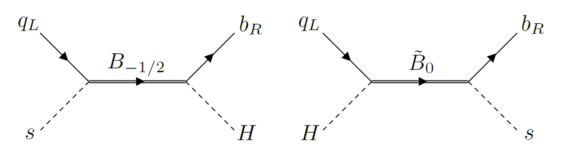
The FN mechanism can also be expressed through the “spaghetti diagrams”, which looks like a 2 to 2 scattering in this case with only one flavon inserted. Spaghetti diagrams that generate the suppressed bottom quark mass are shown in Fig. 1. These diagrams give us the bottom mass we expect after integrating out the heavy Froggatt-Nielsen fields, which are composite fermionic resonances in this model, and replacing the scalar fields with their VEVs.

So far, we see two different flavor charge assignments for the right-handed bottom quark, which lead to two different bottom Yukawa coupling terms. Both of them successfully generate a suppressed bottom Yukawa coupling through the FN mechanism. The difference between these two cases is listed in Table  1.

Here we assume the flavor charge of $q_{L}$ is 1/2 and $t_{R}$ is 0, such that the top quark mass comes from $H_{2}$. We can see the two cases represent different signs of $\Delta_{b}$. It will affect the way we extend our model to include lighter quarks, which will be discussed next. The difference between the types of 2HDM results in different Higgs phenomenology. The second Higgs doublet is expected to be the main target among the exotic states in the model. The results of the direct searches will be shown in the next section. The factor of suppression is also related to the experimental constraint. The smaller $\epsilon$ required for the correct mass ratio implies a smaller VEV $v_{s}$ of the flavon field, which will end up with a larger deviation in flavor observables and thus is strongly constrained.

As yet, we only get the hierarchy between the top and bottom quarks, which belong to the third generation. To include the lighter quarks, more suppression is needed, which means more insertion of the flavon field $s$ and a larger difference in flavor charges. This will require the lighter quarks to be embedded in even larger representations.

Take case (1) for example. We have already gotten the flavor charges of the third generation quarks. To extend to the first and the second generations, one possible flavor charges assignment ³³ 3 The assignment is borrowed from Eq. (2.15) of Bauer et al. 2015. The resulting mass ratios and CKM matrix can partially reproduce observed values with $\mathcal{O}(1)$ correction. is listed in Table 2. It implies that we need even larger representations to have flavor charges different by $7/2$. That would require representations with more than 4 indices for the quark sector.

For case (2), it is more difficult to get a consistent flavor charges assignment for the desired CKM matrix. For the flavor charge of the third generation quarks, we find that they follow the order $[b_{R}]>[q_{L}]>[t_{R}]$, which is also applied to the extension. From the relation, the left-handed quarks should always sit in the middle. This requirement restricts the flavor charge difference we can have. For example, $q_{1,L}$ and $q_{2,L}$ can only be either $1/2$ or $3/2$, which will lead to unsuppressed entries in the CKM matrix. Therefore, considering the flavor charge assignment for the light quarks, case (1) is preferred over case (2). However, we will still discuss the constraints on parameter space of case (2) assuming that it can generate a similar Yukawa matrix as case (1).

The exact embedding will be explored in future work. To discuss the experimental constraints of flavons in the following section, we will assume this mechanism can be extended to all the generations and is responsible for all the light quark masses in both cases. Also, for flavon phenomenology, the results are mainly determined by two parameters, the flavon mass $M_{s}$ and the flavon VEV $v_{s}$.

The phenomenology of 2HDM has been well-studied, and we can directly borrow the results from Kling et al. 2020. For case (2) as a Type-I 2HDM, there is no further constraint since the second Higgs doublet is decoupled from the fermion sector. But for case (1), a Type-II 2HDM, the constraints are important because the suppression of the bottom mass comes partially from the FN mechanism and partially from tan$\beta$. Therefore, the value of tan$\beta$ will decide the $\epsilon$ we need from the FN mechanism. The strongest constraint for a Type-II 2HDM comes from the $\tau\tau$ search, which restricts tan$\beta<6-10$ for a wide mass scale. If we make it a Flipped 2HDM instead, where the charged leptons get masses from $H_{2}$ instead of $H_{1}$, the coupling between heavy Higgs and $\tau\tau$ will become much smaller. Then the main constraint comes from $\bar{b}b$ search, and tan$\beta\sim 20$ is still allowed. However, we would like to stick to a normal Type-II 2HDM for case (1) and set the benchmark with

for the following discussion.

The physical flavon fields include a scalar component $s$ and a pseudoscalar component $a$. The masses of two types of flavons depend on the complete flavon potential, which is discussed in the appendix B. If flavor symmetry is exact and spontaneously broken by flavor symmetry conserving potential, then the pseudoscalar flavon should be massless, which is not acceptable. Therefore, the explicit breaking of flavor symmetry in the flavon potential is needed. For simplicity, we will assume the mass of scalar, $M_{s}$, and the mass of pseudoscalar, $M_{a}$, are the same. This spectrum can be achieved if flavor symmetry is broken by a tadpole term in the flavon potential as shown in appendix B. Therefore, from now on, we will use flavon $s$ for both the scalar and pseudoscalar components and $M_{s}$ for the flavon mass, which is expected to be at the sub-TeV scale.

The production and decay of flavons have already been comprehensively discussed in Tsumura and Velasco-Sevilla 2010; Bauer et al. 2016b. Although the flavon coupling terms in these papers might look different from ours, the exact values are determined by the observed quark masses and the CKM matrix. Therefore, the flavon couplings with the form $m/v_{s}$ should have similar values in all kinds of flavon models up to an $\mathcal{O}(1)$ factor. The numerical values in these two sections are derived based on their analysis with additional adjustments from our setup.

The main production for sub-TeV flavons come from the single production process $b\bar{b}\to s$. The cross section for flavons with $M_{s}=500$ GeV is

in 14 TeV LHC. Taking $v_{s}=150$ GeV, around $2.2\times 10^{4}$ flavons will be produced in the HL-LHC era with an integrated luminosity of 3 ab^-1. In case (2) with smaller $v_{s}$, the number is multiplied by a factor of 36.

The decay branching ratios for flavons are independent of $v_{s}$ but only depend on the flavor structure. If flavons only couple to the third generation, the dominate decay channel will be $b\bar{b}$ channel and $\tau\tau$ channel with roughly $\sim 85\%$ and $\sim 15\%$ branching ratio. If the FN mechanism is extended to all SM particles and responsible for the full Yukawa matrix, then there will be exotic final states like $tc$ and $tu$. It turns out that the $tc$ channel will be the dominant one due to the large mixing required to reproduce the desired CKM matrix. The ratios depend on tan$\beta$, too. Under the benchmark values, we get the branching ratios for each channels as $tc~(96.8\%)$, $b\bar{b}~(2.7\%)$, and $\tau\tau~(0.5\%)$. However, the hadronic channels suffer from large backgrounds. The leptonic channel can reach $\sigma\times BR\sim 10^{-3}$ pb for sub-TeV flavon in HL-LHC, but it is still above the benchmark value. The discovery can be made in a future 100 TeV collider, where the cross section is expected to be $\sim 100$ times larger, and the integrated luminosity is also higher. In that case, the distinct $tc$ channel search will provide strong evidence for the origin of the Yukawa matrix.

The top partners in the $SU(6)/Sp(6)$ CHM are vector-like fermionic resonances that form a sextet of the $Sp(6)$ global symmetry. Their quantum numbers under the SM gauge symmetry are $(3,2,1/6)[\times 2]$, $(3,1,2/3)$, and $(3,1,-1/3)$, which are identical to those of the SM quarks. There are no exotic states with higher or lower hypercharges. These states are degenerate in the limit of unbroken $Sp(6)$ global symmetry. Only small splittings arise from the explicit symmetry breaking effects. Their mass $M_{T}\sim g_{T}f$ plays the important role of cutting off the quadratic contribution from the top quark loop to the Higgs potential. The generic expectation of the composite fermionic resonances is $M_{F}=5-10$ TeV with $g_{F}=5-10$. However, naturalness prefers a smaller $M_{T}$ to minimize the required fine-tuning, which usually requires $g_{T}\gtrsim 1$. The current bound on the top partner mass has reached $\sim 1.2$ TeV Sirunyan et al. 2018; Aaboud et al. 2018. The HL-LHC can further constrain the mass up to $\sim 1.5$ TeV Cid Vidal et al. 2019. A future 100 TeV collider will cover the entire interesting mass range of the top partners if no severe tuning conspires.

For the bottom partners, they form a $\mathbf{14}_{-1/3}\oplus\mathbf{1}_{-1/3}$ under $Sp(6)$ global symmetry. The quantum numbers for the total of 15 fields under the SM gauge group are $(3,2,1/6)[\times 2]$, $(3,2,-5/6)[\times 2]$, $(3,1,-1/3)[\times 4]$, and $(3,3,-1/3)$, which include exotic resonances with EM charge $-4/3$. The states are not degenerate, and the singlet is expected to be lighter. The masses of the bottom partners $M_{B}\sim g_{B}f$, unlike the top partners, don’t have a large effect on the fine-tuning due to the small bottom Yukawa coupling. Therefore, they could be around the compositeness scale with $M_{B}=5-10$ TeV, which is beyond the LHC searches. The heavier $M_{B}\sim g_{B}f$ also leads to additional suppression $g_{T}/g_{B}$ on the mass ratio between the top and bottom quarks, which can relieve the required $\epsilon$ we need.

References

- Chatrchyan et al. (2012) S. Chatrchyan et al. (CMS), Observation of a new boson at a mass of 125 GeV with the CMS experiment at the LHC, Phys. Lett. B716, 30 (2012), arXiv:1207.7235 [hep-ex] .
- Aad et al. (2012) G. Aad et al. (ATLAS), Observation of a new particle in the search for the Standard Model Higgs boson with the ATLAS detector at the LHC, Phys. Lett. B716, 1 (2012), arXiv:1207.7214 [hep-ex] .
- Babu (2010) K. Babu, TASI Lectures on Flavor Physics, in Theoretical Advanced Study Institute in Elementary Particle Physics: The Dawn of the LHC Era (2010) pp. 49–123, arXiv:0910.2948 [hep-ph] .
- Kaplan and Georgi (1984) D. B. Kaplan and H. Georgi, SU(2) x U(1) Breaking by Vacuum Misalignment, Phys. Lett. 136B, 183 (1984).
- Kaplan et al. (1984) D. B. Kaplan, H. Georgi, and S. Dimopoulos, Composite Higgs Scalars, Phys. Lett. 136B, 187 (1984).
- Froggatt and Nielsen (1979) C. Froggatt and H. B. Nielsen, Hierarchy of Quark Masses, Cabibbo Angles and CP Violation, Nucl. Phys. B 147, 277 (1979).
- Bazzocchi et al. (2003) F. Bazzocchi, S. Bertolini, M. Fabbrichesi, and M. Piai, The Little flavons, Phys. Rev. D 68, 096007 (2003), arXiv:hep-ph/0306184 .
- Bazzocchi et al. (2004) F. Bazzocchi, S. Bertolini, M. Fabbrichesi, and M. Piai, Fermion masses and mixings in the little flavon model, Phys. Rev. D 69, 036002 (2004), arXiv:hep-ph/0309182 .
- Bazzocchi and Fabbrichesi (2004) F. Bazzocchi and M. Fabbrichesi, A Heavy Higgs boson from flavor and electroweak symmetry breaking unification, Phys. Rev. D 70, 115008 (2004), arXiv:hep-ph/0407358 .
- Bazzocchi and Fabbrichesi (2005) F. Bazzocchi and M. Fabbrichesi, Flavor and electroweak symmetry breaking at the TeV scale, Nucl. Phys. B 715, 372 (2005), arXiv:hep-ph/0410107 .
- Alanne et al. (2019) T. Alanne, S. Blasi, and F. Goertz, Common source for scalars: Flavored axion-Higgs unification, Phys. Rev. D 99, 015028 (2019), arXiv:1807.10156 [hep-ph] .
- Calibbi et al. (2017) L. Calibbi, F. Goertz, D. Redigolo, R. Ziegler, and J. Zupan, Minimal axion model from flavor, Phys. Rev. D 95, 095009 (2017), arXiv:1612.08040 [hep-ph] .
- Ema et al. (2017) Y. Ema, K. Hamaguchi, T. Moroi, and K. Nakayama, Flaxion: a minimal extension to solve puzzles in the standard model, JHEP 01, 096, arXiv:1612.05492 [hep-ph] .
- Bauer et al. (2015) M. Bauer, M. Carena, and K. Gemmler, Flavor from the Electroweak Scale, JHEP 11, 016, arXiv:1506.01719 [hep-ph] .
- Bauer et al. (2016a) M. Bauer, M. Carena, and K. Gemmler, Creating the fermion mass hierarchies with multiple Higgs bosons, Phys. Rev. D 94, 115030 (2016a), arXiv:1512.03458 [hep-ph] .
- Low et al. (2002) I. Low, W. Skiba, and D. Tucker-Smith, Little Higgses from an antisymmetric condensate, Phys. Rev. D66, 072001 (2002), arXiv:hep-ph/0207243 [hep-ph] .
- Cai et al. (2019) C. Cai, G. Cacciapaglia, and H.-H. Zhang, Vacuum alignment in a composite 2HDM, JHEP 01, 130, arXiv:1805.07619 [hep-ph] .
- Cheng and Chung (2020) H.-C. Cheng and Y. Chung, A More Natural Composite Higgs Model, JHEP 10, 175, arXiv:2007.11780 [hep-ph] .
- Peccei and Quinn (1977) R. Peccei and H. R. Quinn, Constraints Imposed by CP Conservation in the Presence of Instantons, Phys. Rev. D 16, 1791 (1977).
- (20) In fact, this global symmetry is more similar to the Peccei-Quinn (PQ) symmetry Peccei and Quinn 1977. Models that identify as flavor symmetry had been studied in axiflavon models Calibbi et al. 2017; Ema et al. 2017. However, in this paper, we will not deal with the strong CP problem and axions, so we would like to call it flavor symmetry.
- Kaplan (1991) D. B. Kaplan, Flavor at SSC energies: A New mechanism for dynamically generated fermion masses, Nucl. Phys. B365, 259 (1991).
- Glashow and Weinberg (1977) S. L. Glashow and S. Weinberg, Natural Conservation Laws for Neutral Currents, Phys. Rev. D 15, 1958 (1977).
- Paschos (1977) E. Paschos, Diagonal Neutral Currents, Phys. Rev. D 15, 1966 (1977).
- (24) We consider the running of quark masses up to 1 TeV Xing et al. 2008, which gives . The ratio might be larger because the VEV of the flavon field is below the TeV scale.
- Xing et al. (2008) Z.-z. Xing, H. Zhang, and S. Zhou, Updated Values of Running Quark and Lepton Masses, Phys. Rev. D 77, 113016 (2008), arXiv:0712.1419 [hep-ph] .
- (26) The assignment is borrowed from Eq. (2.15) of Bauer et al. 2015. The resulting mass ratios and CKM matrix can partially reproduce observed values with correction.
- Kling et al. (2020) F. Kling, S. Su, and W. Su, 2HDM Neutral Scalars under the LHC, JHEP 06, 163, arXiv:2004.04172 [hep-ph] .
- Tsumura and Velasco-Sevilla (2010) K. Tsumura and L. Velasco-Sevilla, Phenomenology of flavon fields at the LHC, Phys. Rev. D 81, 036012 (2010), arXiv:0911.2149 [hep-ph] .
- Bauer et al. (2016b) M. Bauer, T. Schell, and T. Plehn, Hunting the Flavon, Phys. Rev. D 94, 056003 (2016b), arXiv:1603.06950 [hep-ph] .
- Sirunyan et al. (2018) A. M. Sirunyan et al. (CMS), Search for vector-like T and B quark pairs in final states with leptons at 13 TeV, JHEP 08, 177, arXiv:1805.04758 [hep-ex] .
- Aaboud et al. (2018) M. Aaboud et al. (ATLAS), Combination of the searches for pair-produced vector-like partners of the third-generation quarks at 13 TeV with the ATLAS detector, Phys. Rev. Lett. 121, 211801 (2018), arXiv:1808.02343 [hep-ex] .
- Cid Vidal et al. (2019) X. Cid Vidal et al., Report from Working Group 3, CERN Yellow Rep. Monogr. 7, 585 (2019), arXiv:1812.07831 [hep-ph] .
- (33) LHCb-Collaboration, New results on theoretically clean observables in rare B-meson decays from LHCb, https://indico.cern.ch/event/976688/ .
- Grinstein and Wise (1988) B. Grinstein and M. B. Wise, Weak Radiative B Meson Decay as a Probe of the Higgs Sector, Phys. Lett. B 201, 274 (1988).
- Hou and Willey (1988) W.-S. Hou and R. S. Willey, Effects of Charged Higgs Bosons on the Processes , and , Phys. Lett. B 202, 591 (1988).
- Rizzo (1988) T. G. Rizzo, in the Two Higgs Doublet Model, Phys. Rev. D 38, 820 (1988).
- Geng and Ng (1988) C. Geng and J. N. Ng, Charged Higgs Effect in Mixing, Neutrino Anti-neutrino Decay and Rare Decays of Mesons, Phys. Rev. D 38, 2857 (1988), [Erratum: Phys.Rev.D 41, 1715 (1990)].
- Barger et al. (1990) V. D. Barger, J. Hewett, and R. Phillips, New Constraints on the Charged Higgs Sector in Two Higgs Doublet Models, Phys. Rev. D 41, 3421 (1990).
- Grinstein et al. (1990) B. Grinstein, R. P. Springer, and M. B. Wise, Strong Interaction Effects in Weak Radiative Meson Decay, Nucl. Phys. B 339, 269 (1990).
- Arbey et al. (2018) A. Arbey, F. Mahmoudi, O. Stal, and T. Stefaniak, Status of the Charged Higgs Boson in Two Higgs Doublet Models, Eur. Phys. J. C78, 182 (2018), arXiv:1706.07414 [hep-ph] .
- Misiak and Steinhauser (2017) M. Misiak and M. Steinhauser, Weak radiative decays of the B meson and bounds on in the Two-Higgs-Doublet Model, Eur. Phys. J. C77, 201 (2017), arXiv:1702.04571 [hep-ph] .