The YAPFI phase-field implementation

In a spinodally decomposed structure the value of $\kappa$ together with the thermodynamic description determines the width of the transition zone between $\alpha^{\prime}$ and $\alpha^{\prime\prime}$. According to Cahn and Hilliard [5] the width $l$ of the interface is approximately

where $x_{B}^{\alpha^{\prime\prime}}$ and $x_{B}^{\alpha^{\prime}}$, the equilibrium compositions, and $\Delta G_{m}^{max}$ are indicated in Fig. 3.

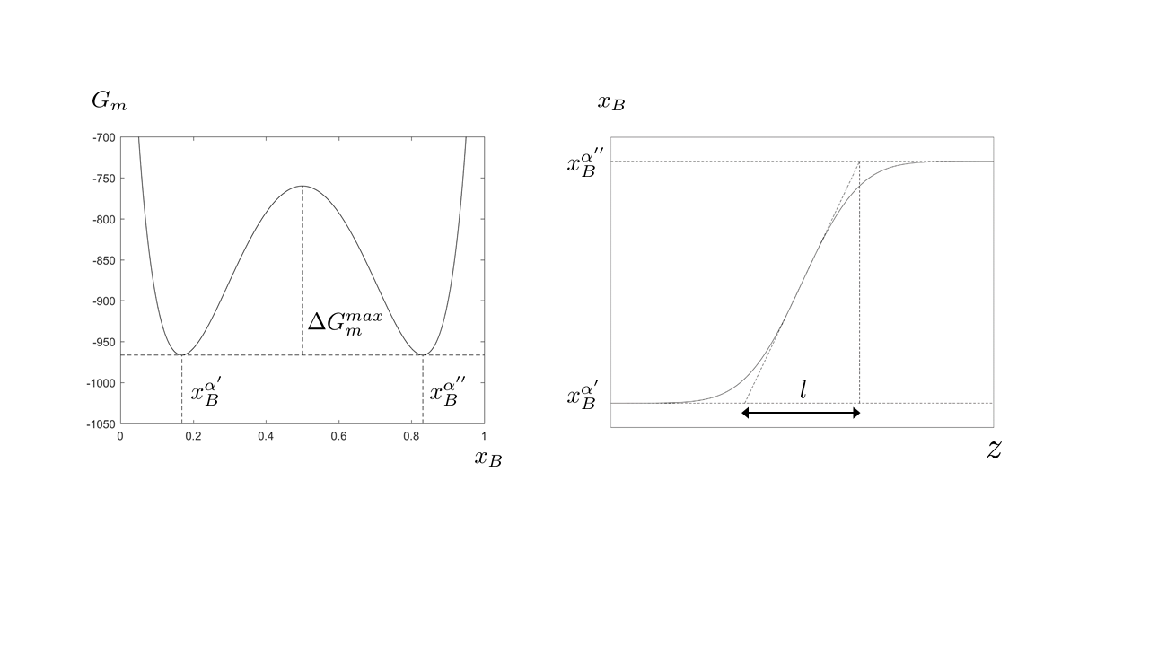
However, the transition between $\alpha^{\prime}$ and $\alpha^{\prime\prime}$ is gradual and the interface is therefore said to be diffuse, see Fig. 3. This is a central concept of the phase-field method, but note that the interface in a spinodally decomposed structure separates regions that differ only in composition (if a single crystal grain is considered), not in structure or orientation.

The treatment by Allen and Cahn is essentially directly applicable to the migration of phase interfaces and grain boundaries. Collins and Levine [11] applied it to solidification of a pure substance including thermal diffusion.

Anisotropic surface energy is an important factor with regards to the evolution of microstructural morphology. Kobayashi [12] considered this when simulating dendritic crystal growth. To incorporate this in a phase field formulation, a gradient energy coefficient $\varepsilon$ was taken to be a function of the gradient of a phase field variable $\phi$, i.e. $\varepsilon\left(\nabla\phi\right)$.

$\phi$ take the value one in the solid and zero in the liquid, $0\leq\phi\leq 1$. See also section 5.2.

The Gibbs energy functional is written as

where $g$ is Gibbs energy per unit volume, $[J/m^{3}]$, $c_{j}$ is concentration of component $j$, $[mol/m^{3}]$. The $\phi_{i}$ are phase field variables, $0\leq\phi_{i}\leq 1$. In general, a specific phase-field variable is associated with a specific phase. Different phase-field variables associated with the same phase generally represent different crystal grains.

In general, $\varepsilon_{ij}<0$.

For convenience we let

where $g_{1}$ is a function of the bulk Gibbs energies of the participating phases and the phase-field variables and $g_{2}$ is a function of composition and the phase-field variables. The derivative $\partial g_{1}/\partial c_{k}$ will then be a function of the bulk chemical potentials of component $k$. The function $g_{2}$ is associated with the interfacial energy and can also be used to introduce Gibbs energy contributions due to specific coupling effects between composition and phase-field variables. Thus,

where $r$ is a phase index and $p^{r}\left(\boldsymbol{\phi}\right)$ is an interpolating polynomial. Though $g_{1}$ is written as a sum over the participating phases, since that is the common form, arbitrary expressions are allowed.

The temporal evolution of composition variable $c_{j}$ is given by a slightly modified Cahn–Hilliard equation [8] in order to take into account the effect of a temperature gradient (see also section 3)

The parameter $Q_{j}^{\star}$ is the so-called heat of transport [9].

The temporal evolution of phase-field variable $\phi_{k}$ is given by the Allen–Cahn equation [10]

With $g_{0}(\mathbf{c},\boldsymbol{\phi},T)$, $\kappa_{ij}(\mathbf{c},\boldsymbol{\phi},T)$ and $\varepsilon_{ij}(\mathbf{c},\boldsymbol{\phi},\nabla\boldsymbol{\phi},T)$ — arbitrary analytical expressions are allowed for $g_{0}$, $\boldsymbol{\kappa}$ and $\boldsymbol{\varepsilon}$ — the variational derivatives are evaluated as

where the vector quantity $\boldsymbol{\xi}_{k}=[\xi_{kx}\,\xi_{ky}\,\xi_{kz}]$ was introduced for convenience

It should be noted that when taking the derivatives $\partial/\partial(\nabla c_{k})$ and $\partial/\partial(\nabla\phi_{k})$ the result is a vector, e.g.

$\nabla\cdot(\sum_{i}\nabla\phi_{i}\sum_{j}\cdot\nabla\phi_{j}[\partial\varepsilon_{ij}/\partial(\nabla\phi_{k})])$ is scalar.

All derivatives are evaluated analytically.

Fourier’s law yields the heat flux $J_{q}$

where $\lambda$ is the thermal conductivity.

The heat flux is combined with a conservation law

where $\dot{q}$ is a source term. If only isobaric conditions are considered $Q$ equals volumetric enthalpy.

The relation between $\partial Q/\partial t$ and $\partial T/\partial t$ is

The source term $\dot{q}$ is given by

The final expression is

In the formal description above concentration $c_{k}$ $[mol/m^{3}]$ is used, but internally the software is mainly using mole fractions $x_{k}$, which is reflected in the required format of input data.

When entering data, the function $g_{1}$ is allowed to be an arbitrary function of the molar Gibbs energies of the participating phases $G_{m}^{\alpha}$ and the phase-field variables $\phi_{k}$. The $G_{m}^{\alpha}$ $[J/mol]$ should, in principle, be valid for a microscopically homogeneous single phase system.

The function $g_{2}$ is allowed to be an arbitrary function of R, T the mole fractions of elements $x_{j}$ and the phase-field variables $\phi_{k}$. As $g_{1}$, the input unit of $g_{2}$ is $[J/mol]$.

The gradient energy coefficients $\varepsilon_{ij}$ and $\kappa_{ij}$ are allowed to be arbitrary functions of R, T the mole fractions of element $x_{j}$ and the phase-field variables $\phi_{k}$. In addition, $\varepsilon_{ij}$ may be a function of the gradients of the phase-field variables $\nabla\phi_{k}$, though in general the function should then be formulated such that it is a function of the normal of phase-field variables $\hat{n}_{k}=\nabla\phi_{k}/|\nabla\phi_{k}|$.

The unit of input functions $\varepsilon_{ij}$ and $\kappa_{ij}$ is $[J\cdot m^{2}\cdot mol^{-1}]$.

$M_{\phi}$ should be input with unit $[mol\cdot J^{-1}\cdot s^{-1}]$ whereas $M_{k}$ has unit $[m^{2}\cdot mol\cdot J^{-1}\cdot s^{-1}]$. In the formal description the unit of $M_{\phi}$ is $[m^{3}\cdot J^{-1}\cdot s^{-1}]$, i.e. it differs by a factor $1/V_{m}$ from the required unit of input data.

With the exception of analytical expressions entered for $G_{m}$, the interdependece of $x_{i}$, $\phi_{i}$ and $\nabla\phi_{i}$, respectively, is taken into account when evaluating partial derivatives with respect to these variables. The exception made for $G_{m}$ is due to the fact that this is not necessary when evaluating chemical potentials from $G_{m}$ and $\partial G_{m}/\partial x_{i}$.

The total interfacial energy of a system $E^{int}$ $[J]$ is typically given by

The “primes” have been added to indicate that the units here are those required in the input, i.e. $[J/mol]$ and $[J\cdot m^{2}\cdot mol^{-1}]$ for $g_{2}^{\prime}$ and $\varepsilon_{ij}^{\prime}$, respectively.

Growth of a phase $\alpha$ from a supersaturated parent $\beta$ phase was considered for a hypothetical binary system. Both phases are regular solutions. A corresponding sharp interface simulation using Dictra [21] was performed.

For this simulation the $g_{2}$ phase interface Gibbs energy contribution was given by the method suggested by Finel et al. [22]. That method has the advantage that it allows for very thin phase interfaces, i.e. extending over very few grid points.

Concentration profiles at different times are shown in Fig. 4. The profiles obtained from Dictra are shown with dotted lines. The agreement is very satisfactory and could of course be even better with a denser grid.

For simplicity only 2D simulations will be considered. Following Kobayashi [12], let

where $\bar{\varepsilon}$ is a mean surface energy and

The normal vector at the interface is given by

Let the reference direction point in the positive x direction, then,

Results from simulations using different values of $\delta$ are shown in Fig. 5. The same hypothetical A-B system as in section 5.1 was considered, and, again, growth of $\alpha$ from supersaturated $\beta$ was simulated.

As stated above, $\varepsilon$ can be an arbitrary analytical function of $\mathbf{c}$, $\boldsymbol{\phi}$ and $\nabla\boldsymbol{\phi}$. When setting up the simulation and entering the expression for $\varepsilon$, the derivatives $\partial\phi/\partial x$ and $\partial\phi/\partial y$ are thus two of the allowed variables.

In Fig. 6 are shown results from a 3D simulation of spinodal decomposition. The simulation was performed for a hypothetical A-B-C system consisting of a single regular solution phase in which all regular solution parameters $L_{ij}>0$, but with different values. The domain size was $\left(25\cdot 10^{-9}\right)^{3}\,\left[\text{m}^{3}\right]$ with $100^{3}$ grid points. Periodic boundary conditions were applied. The gradient energy coefficients were set to $\kappa_{ij}=-d^{2}L_{ij}/2$ where d is the grid spacing, i.e. $0.25\,\text{nm}$. Initial mole-fractions were $x_{A}=x_{B}=0.33,\,x_{C}=0.34$ with a random noise in the range $\pm 0.01$.

For an example of a 2D simulation using the homogenization model the reader is referred to the work by Salmasi et al. [23]. In that work geometry effects during gradient sintering of cemented carbides was investigated.

References

- [1] L-Q Chen, Annual Review of Materials Research 32(2002)113-140.
- [2] I Singer-Loginova, HM Singer, Reports on Progress in Physics 71(2008)106501
- [3] N Moelans, B Blanpain, P Wollants, CALPHAD 32(2008)268.
- [4] R Becker, Annalen der Physik 32(1938)128-140.
- [5] JW Cahn, JE Hilliard, Journal of Chemical Physics 28(1958)258-267.
- [6] M Hillert, thesis, Massachusetts Institute of Technology, 1956.
- [7] M Hillert, Acta Metallurgica 9(1961)525-535.
- [8] JW Cahn, Acta Metallurgica 9(1961)795.
- [9] FA Nichols, Journal of Nuclear Materials 84(1979)1.
- [10] SM Allen, JW Cahn, Acta Metatllurgica 27(1979)1085.
- [11] JB Collins, H Levine, Physcial Review B 31(1985)6119-6122.
- [12] R Kobayashi, Physica D 63(1993)410-423.
- [13] AA Wheeler, WJ Boettinger, GB McFadden, Physical Review E 45(1992)7424-7440.
- [14] AA Wheeler, WJ Boettinger, GB McFadden, Physical Review E 47(1993)1893-1909.
- [15] H Larsson, A Engström, Acta Materialia 54(2006)2431.
- [16] H Larsson, L Höglund, CALPHAD 33(2009)495.
- [17] A Engström, L Höglund, J Ågren, Metallurgical and Materials Transactions A 29A(1994)1127.
- [18] J Morral, BM Dupen, CC Law, Metallurgical Transactions A 23A(1992)2069.
- [19] J-O Andersson, T Helander, L Höglund, P Shi, B Sundman, Calphad 26(2002)273-312.
- [20] H Larsson, L Höglund, CALPHAD 50(2015)1-5.
- [21] A Borgenstam, A Engström, L Höglund, J Ågren, Journal of Phase Equilibria 21(2000)269
- [22] A Finel, Y Le Bouar, B Dabas, B Appolaire, Y Yamada, T Mohri, Physical Review Letters 121(2018)025501.
- [23] A Salmasi, A Blomqvist, H Larsson, Results in Materials 1(2019)100008