Backup Control Barrier Functions: Formulation and Comparative Study

We begin by a brief review of control barrier functions. Consider the following control affine system:

where $x$ is the system state and $u$ is the input. Suppose there exists a function $h:\mathbb{R}^{n}\to\mathbb{R}$ that satisfies

where $\mathcal{X}_{0}$ is the set of initial states and $\mathcal{X}_{d}$ is the danger set that we want to keep the state away from. $\alpha(\cdot)$ is a class-$\mathcal{K}$ function, i.e., $\alpha(\cdot)$ is strictly increasing and satisfies $\alpha(0)=0$. Then $h$ is called control barrier function, and for any legacy controller, the CBF controller is a supervisory controller that enforces the state to stay inside $\left\{{x\mid h(x)\geq 0}\right\}$ with the following quadratic programming:

where $u^{0}$ is the input of the legacy controller.

The third condition in (2) ensures that (3) is always feasible, yet it is difficult to find an $h$ that satisfies it. For clarity, we refer to a function that satisfies the first two conditions in (2) a CBF candidate, a function that satisfies all three conditions a valid CBF.

The CBF condition is closely tied to the concept of a control invariant set, which is defined as follows.

It is straightforward to see that for a valid CBF, $\{x|h(x)\geq 0\}$ is a control invariant set. On the other direction, suppose for a CBF candidate $h$, its 0-level set is a control invariant set. Immediately from Definition 1,

otherwise the state will exit $\mathcal{S}$, which contradicts Definition 1. Then $h$ can be shown to be a valid control barrier function by picking an $\alpha$ large enough given some continuity condition (Lipschitz continuity of $h$ and $\dot{h}$). As a result, the third condition in (2) is also referred to as the set invariance condition.

As a motivating example, consider a simple double integrator with

The safety constraint is $X\leq C$ with a constant $C$. Suppose one directly takes the safety constraint as a CBF candidate: $h_{0}(x)=C-s$. There are two issues. First, $h_{0}$ has relative degree 2, i.e., $\dot{h}_{0}$ is not a function of $u$. Second, the set $\{x|h_{0}(x)\geq 0\}$ is not control invariant. Consider the case where $s=C,v>0$, the limited input cannot stop the state from crossing into the danger set due to inertia.

For this simple system, it is widely known that a simple valid CBF exists:

which is the safety constraint combined with the minimum stopping distance. When $h(x)\geq 0$, one can always apply the maximum deceleration $u=-u_{\max}$ until $v=0$ and the safety constraint remains satisfied. Fig. 1 shows the difference between $h$ and $h_{0}$ where $h_{0}$ includes a part of the state space from which the safety constraint will eventually be violated.

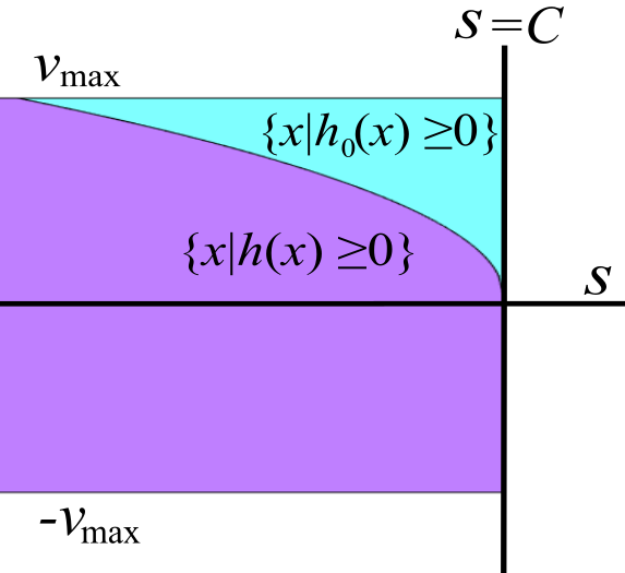
In fact, the above CBF is exactly the backup CBF with the backup policy being

We shall show later that the backup policy $\pi$ takes the system to a small control invariant set $\mathcal{S}_{0}=\{x|v=0\}$, and $\{x|h(x)\geq 0\}$ with $h$ in (4) is the set of initial conditions that can be brought to $\mathcal{S}_{0}$ while satisfying the safety constraint. In this view, $h$ is induced from the backup policy $\pi$.

As mentioned in the Introduction, computing a control invariant set is very difficult, especially for high-dimensional nonlinear systems. We shall show that for complicated dynamic systems, a valid CBF can be fairly easily obtained from a backup policy. Though the CBF induced from a backup policy might not have the nice closed form as in the double integrator case, the CBF QP can be solved online and is guaranteed to be feasible.

Before going into the detail, some important notations are reviewed. Given the dynamic system in (1), a control policy $\pi:\mathbb{R}^{n}\to\mathcal{U}$, the closed-loop dynamics under $\pi$ is $\dot{x}=f_{\pi}(x)=f(x)+g(x)\pi(x)$. We let $\Pfx:\mathbb{R}^{n}\times(-\infty,\infty)\to\mathbb{R}^{n}$ denote the flow map, i.e., $\Pfx(x_{0},t)$ denotes the solution $x(t_{0}+t)$ to the Initial Value Problem (IVP) at time $t_{0}+t$ with $x(t_{0})=x_{0}$ under the dynamics $f_{\pi}$. Note that since (1) is time invariant, the initial time $t_{0}$ is irrelevant. Moreover, the flow map is additive in $t$:

Since the flow map can be written as

it is differentiable w.r.t. both $t$ and $x$. By inspection, $\frac{\partial\Pfx(x_{0},t)}{\partial t}=f_{\pi}(\Pfx(x_{0},t))$. To obtain the partial derivative over $x_{0}$, take derivative on both sides:

from [16], we can define $Q(t)=\frac{\partial\Pfx(x_{0},t)}{\partial x_{0}}$ as the sensitivity Jacobian, and taking derivative over $t$ on both sides yields

where $x(t)=\Pfx(x_{0},t)$. This fact will play a key role on the derivation of the CBF condition.

The physical interpretation of Proposition 1 is that the flow under the backup strategy $\pi$ would not change with time if the current state follows $\pi$.

Consider a safe region $\mathcal{C}\doteq\{x|h^{\mathcal{C}}\geq 0\}\subseteq\mathbb{R}^{n}$, a control invariant set $\mathcal{S}_{0}\doteq\{x|h^{\mathcal{S}}\geq 0\}\subseteq\mathcal{C}$ with $h^{\mathcal{C}},h^{\mathcal{S}}:\mathbb{R}^{n}\to\mathbb{R}$ differentiable. Given a backup controller $\pi$, define the $T$-time constrained reachable set as

which contains the states from which the flow under $f_{\pi}$ will stay in $\mathcal{C}$ and reach $\mathcal{S}_{0}$ by $T$. The theoretical root of the backup CBF approach is the following simple observation.

The proof can be found in [17], we provide a brief proof for completeness.

Fig. 2 shows theorem 1 pictorially. The yellow square is the state constraint $\mathcal{C}$, given a small known control invariant set $\mathcal{S}_{0}$ (the blue ellipse), all states that can be driven to $\mathcal{S}_{0}$ under $f_{\pi}$ (the closed-loop dynamics under the backup policy $\pi$) while staying inside $\mathcal{C}$ in the meantime forms a larger control invariant set $\mathcal{S}$ shown in brown. Note that the point on the top right is not inside $\mathcal{S}$ because the trajectory under $f_{\pi}$ is not completely contained $\mathcal{C}$.

Regarding the horizon $T$, the following lemma is true.

Lemma 1 states that $\mathcal{R}(\mathcal{S}_{0},\mathcal{C},f_{\pi},T)$ monotonically increases with $T$ in the set inclusion sense.

With a control invariant set $\mathcal{S}$ defined, a control barrier function $h$ can be defined.

To implement the CBF $h$, $\dot{h}$ is needed. First $h$ needs to be written as a function of time:

Since $h$ is defined as the minimum of multiple functions, it may not be differentiable. Even in the differentiable case, the CBF condition may turn out to be nonconvex in the control input $u$. Instead, the CBF condition is enforced on every $\tau$, which is a sufficient condition for original CBF condition.

First consider $h^{\mathcal{S}}(\Pfx(x(t),T))$. By the chain rule,

where the sensitivity Jacobian $\frac{\partial\Pfx(x(t),T)}{\partial x}$ can be calculated with (7). The computation of $h^{\mathcal{C}}(\Phi_{f_{\pi}}(x(t)),\tau-t)$ is slightly different:

where $\dot{x}=(f(x(t))+g(x(t))u(t))$. By Proposition 1, $\frac{d\Pfx(x(t),\tau-t)}{dt}|_{u=\pi(x)}=0$, indicating that $\frac{dh^{\mathcal{C}}(\Pfx(x(t),\tau-t))}{dt}=0$ if $u(t)=\pi(x(t))$.

The CBF condition is $\dot{h}+\alpha(h)\geq 0$. We shall impose this condition on $h^{\mathcal{S}}(\Pfx_{f_{\pi}}(x,T))$ and $h^{\mathcal{C}}(\Pfx_{f_{\pi}}(x,\tau-t))$ for every $\tau\in[t,t+T]$ instead of only on the $\tau$ minimizing $h^{\mathcal{C}}(\Pfx_{f_{\pi}}(x,\tau-t))$, and the CBF QP is then

In practice, $\mathop{\min}\limits_{\tau\in[t,t+T]}h^{\mathcal{C}}(\Phi_{f_{\pi}}(x(t)),\tau-t)$ may be difficult to evaluate, so a finite set of $t=\tau_{0}<\tau_{1}...<\tau_{N}=t+T$ is used instead of $[t,t+T]$, and the approximation error can be bounded given the Lipschitz constants of the flow map.

Another benefit of the backup CBF is that it is always relative degree one given the system is weakly locally controllable. To show this, we first review some definitions.

We cannot show that the CBF defined in (10) has relative degree 1 due to the $\min$ function over $t\in[0,T]$, however, note that the constraints in the CBF QP in (12) are on all $h^{\mathcal{C}}\circ\Pfx(x,\tau-t)$ with $\tau\in[t,t+T]$ and $h^{\mathcal{S}}\circ\Pfx(x,T)$. Therefore, as long as $h^{\mathcal{S}}$ and $h^{\mathcal{C}}$ are not constant for any subset with a non-empty interior, the CBF QP can be solved as if $h$ has relative degree 1.

Theorem 3 shows that the backup CBF is sufficient without any high order extension or backstepping, it naturally bridges the potentially high relative degree functions $h^{\mathcal{C}}$ and $h^{\mathcal{S}}$ with the input dynamics via the flow map.

To demonstrate the result, a simple lane keeping problem under Dubin’s car model is considered:

where the state $x$ consists of lateral position $Y$, velocity $v$, and heading angle $\psi$, and the input consists of acceleration $a$ and yaw rate $r$, The state constraint considered is $\mathcal{C}=\{|Y|\leq Y_{\max}\wedge|\psi|\leq\psi_{\max}\}$ with $Y_{\max}=1.8m,\psi_{\max}=\pi/3$, and $\mathcal{U}=\{a,r||a|\leq a_{\max}\wedge|r|\leq r_{\max}\}$.

The backup policy is chosen as

where $\Sat$ is the saturation function, $k_{v}>0$ is a constant and $k_{y}$ is calculated via LQR. Under the same controller $\pi$, a CBF is synthesized with the following SOS program:

with $Q(x)\doteq\hat{x}^{\intercal}Q\hat{x}$, and $\hat{x}=[Y,v-v_{des},\psi]^{\intercal}$, where $Q$ is a PSD matrix. $\Sigma[x]$ is the set of sum-of-squares polynomial of $x$, $s_{1},s_{2},s_{3}$ are SOS multipliers for the Positivstellensatz procedure that enforces positive definiteness of a polynomial on a semialgebraic set. Due to the cross product term in line 2, (15) cannot be directly solved via SOS, a line search is used to find the largest $R$ that renders the SOS program feasible. $R^{0}$ is a radius that contains the region of state space we are interested in, (15) essentially tries to fit the largest ball of $Q(x)$ inside $\{h(x)\geq 0\}$ where $h$ is the CBF that satisfies (2). For simplicity, $\sin\psi\approx\psi-\psi^{3}/3$, and the saturation is lifted, which should lead to a larger control invariant set.

Fig. 3 shows the comparison of the CBF computed with HJ, backup CBF, and SOS where the upper plot shows the 3D surface and the lower plot shows the slicing of the set at $v=5m/s$. As expected, Hamilton Jacobi PDE generates the largest control invariant set, the one from backup CBF is smaller, and the SOS one is the smallest since $h$ is restricted to be a polynomial (4-th order in this case).

Obviously, one can choose a better backup policy and greatly improve the result. For example, if we change $v_{des}=0$, and switch to a more aggressive LQR design, the control invariant set computed from backup CBF is almost identical to the one from Hamilton Jacobi, as shown in Fig. 4.

One classic example in safety-critical control is the aeroplane avoidance with the following dynamics:

where $\Delta X$, $\Delta Y$, and $\Delta\psi$ are the difference of $X,Y$ coordinates and heading angles plane $a$ and $b$, $u$ is the turning rate of plane $a$, $v_{a}$ and $v_{b}$ are their velocities, assumed to be constant.

The backup CBF approach is not good at handling malicious disturbance, therefore we assume that plane $b$ maintains a fixed orientation. The safety constraint is defined as $\Delta X^{2}+\Delta Y^{2}\geq R^{2}$, where $R$ is the minimum distance to maintain between the two planes. Fig. 5 shows the danger set ($\{x|h(x)\leq 0\}$) computed with the HJI PDE and the one computed with a simple backup policy:

The two danger sets are almost identical.

Technically, it is not fair to compare the computation time of the backup CBF approach with the benchmarks as the former does not require any offline computation while the online computation is more complicated than normal CBF QP, while CBF based on explicit control invariant set requires computing the control invariant set offline.

Table I shows the computation time of the CBF QP with CBF constructed by the HJ PDE, SOS, and the backup CBF approach. The computation time for backup CBF consists of two parts, the integration of the backup policy, and the CBF QP. As shown by the result, the majority of solver time is spent on the CBF QP, which is 1 magnitude larger than the time used to solve the CBF QP with explicit form. This is mainly because (12) enforces the CBF condition on every $\tau\in[t,t+T]$ (replaced with a sequence of $\tau_{i}$ in practice), which significantly increases the number of constraints. The integration time is relatively small compared to the QP time and can be further reduced. For instance, [21] uses a Koopman operator approach to further simplify the online integration. We also apply the backup CBF on a 16-dimensional quadrotor model, which is way beyond the limit of HJ (maximum dimension 4-5) and SOS (maximum dimension around 8-10), and the backup CBF can still be implemented with a reasonable loop rate.

References

- [1] A. D. Ames, J. W. Grizzle, and P. Tabuada, “Control barrier function based quadratic programs with application to adaptive cruise control,” in 53rd IEEE Conference on Decision and Control. IEEE, 2014, pp. 6271–6278.
- [2] P. Wieland and F. Allgöwer, “Constructive safety using control barrier functions,” IFAC Proceedings Volumes, vol. 40, no. 12, pp. 462–467, 2007.
- [3] J.-P. Aubin, A. M. Bayen, and P. Saint-Pierre, Viability theory: new directions. Springer Science & Business Media, 2011.
- [4] D. Bertsekas, “Infinite time reachability of state-space regions by using feedback control,” IEEE Transactions on Automatic Control, vol. 17, no. 5, pp. 604–613, 1972.
- [5] F. Blanchini, “Set invariance in control,” Automatica, vol. 35, no. 11, pp. 1747–1767, 1999.
- [6] S. Rakovic, P. Grieder, M. Kvasnica, D. Mayne, and M. Morari, “Computation of invariant sets for piecewise affine discrete time systems subject to bounded disturbances,” in 2004 43rd IEEE Conference on Decision and Control (CDC)(IEEE Cat. No. 04CH37601), vol. 2. IEEE, 2004, pp. 1418–1423.
- [7] Y. Chen, H. Peng, J. Grizzle, and N. Ozay, “Data-driven computation of minimal robust control invariant set,” in 2018 IEEE Conference on Decision and Control (CDC). IEEE, 2018, pp. 4052–4058.
- [8] M. Korda, D. Henrion, and C. N. Jones, “Convex computation of the maximum controlled invariant set for polynomial control systems,” SIAM Journal on Control and Optimization, vol. 52, no. 5, pp. 2944–2969, 2014.
- [9] I. M. Mitchell, A. M. Bayen, and C. J. Tomlin, “A time-dependent hamilton-jacobi formulation of reachable sets for continuous dynamic games,” IEEE Transactions on automatic control, vol. 50, no. 7, pp. 947–957, 2005.
- [10] A. Taylor, A. Singletary, Y. Yue, and A. Ames, “Learning for safety-critical control with control barrier functions,” in Learning for Dynamics and Control. PMLR, 2020, pp. 708–717.
- [11] L. Lindemann and D. V. Dimarogonas, “Control barrier functions for signal temporal logic tasks,” IEEE control systems letters, vol. 3, no. 1, pp. 96–101, 2018.
- [12] Q. Nguyen and K. Sreenath, “Exponential control barrier functions for enforcing high relative-degree safety-critical constraints,” in 2016 American Control Conference (ACC). IEEE, 2016, pp. 322–328.
- [13] X. Xu, “Constrained control of input–output linearizable systems using control sharing barrier functions,” Automatica, vol. 87, pp. 195–201, 2018.
- [14] W. Xiao and C. Belta, “Control barrier functions for systems with high relative degree,” in 2019 IEEE 58th Conference on Decision and Control (CDC). IEEE, 2019, pp. 474–479.
- [15] T. Gurriet, M. Mote, A. Singletary, P. Nilsson, E. Feron, and A. D. Ames, “A scalable safety critical control framework for nonlinear systems,” IEEE Access, vol. 8, pp. 187 249–187 275, 2020.
- [16] H. Seywald and R. Kumar, “Desensitized optimal trajectories,” Analytical Mechanics Associates Rept, pp. 03–16, 2003.
- [17] T. Gurriet, M. Mote, A. D. Ames, and E. Feron, “An online approach to active set invariance,” in 2018 IEEE Conference on Decision and Control (CDC). IEEE, 2018, pp. 3592–3599.
- [18] R. Hermann and A. Krener, “Nonlinear controllability and observability,” IEEE Transactions on automatic control, vol. 22, no. 5, pp. 728–740, 1977.
- [19] X. Xu, J. W. Grizzle, P. Tabuada, and A. D. Ames, “Correctness guarantees for the composition of lane keeping and adaptive cruise control,” IEEE Transactions on Automation Science and Engineering, vol. 15, no. 3, pp. 1216–1229, 2017.
- [20] Y. Chen, A. Hereid, H. Peng, and J. Grizzle, “Enhancing the performance of a safe controller via supervised learning for truck lateral control,” Journal of Dynamic Systems, Measurement, and Control, vol. 141, no. 10, 2019.
- [21] C. Folkestad, Y. Chen, A. D. Ames, and J. W. Burdick, “Data-driven safety-critical control: Synthesizing control barrier functions with koopman operators,” IEEE Control Systems Letters, 2020.