Statistical properties of the localization measure of chaotic eigenstates and the spectral statistics in a mixed-type billiard
Abstract
We study the quantum localization in the chaotic eigenstates of a billiard with mixed-type phase space (J. Phys. A: Math. Gen. 16, 3971 (1983); 17, 1049 (1984)), after separating the regular and chaotic eigenstates, in the regime of slightly distorted circle billiard where the classical transport time in the momentum space is still large enough, although the diffusion is not normal. This is a continuation of our recent papers (Phys. Rev. E 88, 052913 (2013); 98, 022220 (2018)). In quantum systems with discrete energy spectrum the Heisenberg time , where is the mean level spacing (inverse energy level density), is an important time scale. The classical transport time scale (transport time) in relation to the Heisenberg time scale (their ratio is the parameter ) determines the degree of localization of the chaotic eigenstates, whose measure is based on the information entropy. We show that is linearly related to normalized inverse participation ratio. The localization of chaotic eigenstates is reflected also in the fractional power-law repulsion between the nearest energy levels in the sense that the probability density (level spacing distribution) to find successive levels on a distance goes like for small , where , and corresponds to completely extended states. We show that the level repulsion exponent is empirically a rational function of , and the mean (averaged over more than 1000 eigenstates) as a function of is also well approximated by a rational function. In both cases there is some scattering of the empirical data around the mean curve, which is due to the fact that actually has a distribution, typically with quite complex structure, but in the limit well described by the beta distribution. The scattering is significantly stronger than (but similar as) in the stadium billiard (Nonl.Phen.Compl.Sys. 21, No3, 225 (2018)) and the kicked rotator (Phys. Rev. E 91, 042904 (2015)). Like in other systems, goes from to when goes from to . is a function of , similar to the quantum kicked rotator and the stadium billiard.
pacs
01.55.+b, 02.50.Cw, 02.60.Cb, 05.45.Pq, 05.45.MtI Introduction
Quantum chaos (or more generally, wave chaos) deals with phenomena in the quantum domain, which are signatures of the classical chaos in the corresponding classical systems. Stöckmann 1999; Haake 2001; Robnik 2016. The classical dynamics as the ray dynamics of the quantum wave functions is, for example, an analogy of the relationship between the Gaussian ray optics and the wave phenomena of the Maxwell equations describing the electromagnetic field. The classical and the quantum descriptions are connected theoretically through the semiclassical mechanics, which is the short wavelength approximation of the underlying wave field.
In the classically integrable Hamiltonian systems with degrees of freedom the semiclassical theory predicts that the quantum eigenstates (in the -dim phase space, represented by Wigner functions Wigner 1932 or Husimi functions Husimi 1940) are associated with the classical -dim invariant tori. In the case of classical ergodic systems, the eigenstates are microcanonical (uniformly spread over the -dim energy surface). In the case of the mixed-type classical phase space, where regular regions covered by the invariant tori coexist with the chaotic sea (one or more chaotic invariant regions), we have the generic structure (almost all systems are of this type), where we have to distinguish between the quantum regular and irregular (chaotic) eigenstates, an idea proposed qualitatively already in 1973 by Percival Percival 1973. This line of thought lead to the Principle of Uniform Semiclassical Condensation of Wigner functions Robnik 1998, based on work of Berry Berry 1977, Shnirelman Shnirelman 1974, Voros Voros 1979, and further developed by Veble, Robnik and Liu Veble et al. 1999. The Wigner functions of the eigenstates condense uniformly on the classical invariant component in the classical phase space, and this principle (PUSC) has a great predictive power as demonstrated e.g. in Ref. Veble et al. 1999.
The classical dynamics of bounded Hamiltonian systems determines also the statistical properties of the discrete energy spectra of the corresponding eigenstates. For the classically regular motion it predicts Poissonian energy level statistics, while in the classically fully chaotic (ergodic) systems the statistics of Random Matrix Theory (RMT) applies, as conjectured by Bohigas, Giannoni and Schmit Bohigas et al. 1984 in 1984, also by Casati, Valz-Gris and Guarneri Casati et al. 1980, proven by Berry Berry 1985, Sieber and Richter Sieber and Richter 2001, and by Haake and coworkers Müller et al. 2004; Heusler et al. 2004; Müller et al. 2005; Müller et al. 2009, using the semiclassical techniques based on the Gutzwiller’s periodic orbit theory (See Refs. Gutzwiller 1967; Gutzwiller 1969; Gutzwiller 1970; Gutzwiller 1971; Gutzwiller 1980 and also the books by Stöckmann Stöckmann 1999 and Haake Haake 2001).
The intermediate case of the mixed-type Hamilton systems was treated first theoretically by Berry and Robnik Berry and Robnik 1984, and has been analyzed later on in many studies, most accurately by Prosen and Robnik Prosen and Robnik 1999. In this picture the parameter plays the crucial role, being the relative fraction of the phase space volume occupied by the regular regions in the classical phase space, and it also is the relative density of the regular energy levels in the total quantum spectrum of the underlying system. The spectral statistics for the regular levels is Poissonian.
If there are chaotic regions with the relative volume fractions (and corresponding energy level densities) , then for each of them the RMT statistics applies. Usually, the dominant chaotic region is by far the largest one, , so that the smaller chaotic regions can be neglected, and we have .
The best mathematical description of such a mixed-type case is in terms of the gap probability . This is the probability that an energy interval (after unfolding, i.e. reducing the mean energy level density to unity) is empty of levels. Clearly, if regular and chaotic eigenstates are not correlated, being statistically independent of each other, the gap probabiliy simply factorizes, that is
| (1) |
where and refer to the Poissonian and RMT statistics, respectively. The Poissonian is . For the GOE level spacing distribution, which applies if the time reversal symmetry (or any other antiunitary symmetry) exists, the well known Wigner distribution (Wigner surmise) is an excellent analytical approximation
| (2) |
while the corresponding gap probability is
| (3) |
The level spacing distribution is the second derivative of the gap probability , and therefore in this case given by
| (4) | |||||
as derived by Berry and Robnik Berry and Robnik 1984. Of course, . The gap probability is just a special case of probability of finding levels on an interval of length , namely . For more details about the probabilities with see Ref. Prosen and Robnik 1999.
The above statements are correct only if the chaotic states are uniformly extended over the classical invariant chaotic component. This condition, however, is not always satisfied. The phenomenon of dynamical (or quantum) localization can occur, first discovered and further explored by Chirikov, Izrailev and Shepelyansky Chirikov et al. 1981 in the quantum kicked rotator (QKR) introduced by Casati, Chirikov, Izrailev and Ford Casati et al. 1979 as a model system, and later extensively studied in particular by Izrailev Izrailev 1986; Izrailev 1987; Izrailev 1988; Izrailev 1989; Izrailev 1990. The QKR is a time periodic (Floquet) system. The time independent chaotic systems are exemplified by the 2-dim billiard systems. Borgonovi, Casati and Li Borgonovi et al. 1996 have studied from this point of view the stadium billiard of Bunimovich Bunimovich 1979. See also the review by Prosen Prosen 2000. The case of mixed-type billiard has been studied recently by Batistić and Robnik Batistić and Robnik 2010; Batistić and Robnik 2013a; Batistić and Robnik 2013b.
The criterion for localization is in terms of the ratio
| (5) |
of the Heisenberg time and the classical transport time . Here , with being the mean energy level spacing (inverse energy level density), which is an important time scale in any quantum system with discrete energy spectrum, while is the purely classical (-independent) diffusion time, or typical time needed for an ensemble of initial sharply distributed momenta to spread uniformly over the classical chaotic component. If the chaotic eigenstates are maximally localized, while if the eigenstates are maximally extended, but in between we have the partially localized eigenstates. The degree of localization can be measured most easily in terms of the Husimi function Husimi 1940, which is positive definite and can be treated as quasi-probability density. There are three main localization measures: , the information entropy measure, the correlation localization measure, and the normalized inverse participation ratio. As recently shown Batistić and Robnik 2013a; Batistić et al. 2019, they are all proportional to each other (linearly related) and thus equivalent. The energy spectra of the localized chaotic eigenstates can be well described by the fractional power law level repulsion, , for small , and : corresponds to the maximal localization and Poissonian statistics, while corresponds to the maximal extendedness (delocalization) and the RMT statistics. It has been found that is a function of , they are linearly related in QKR and in the stadium billiard, as well as in the present work. It is also an almost rational function of .
The local behaviour of at small can be globalized by approximating it by the well known Brody distribution Brody 1973; Brody et al. 1981, described by the following formula
| (6) |
where by normalization of the total probability and the first moment we have
| (7) |
with being the Gamma function. It interpolates the exponential and Wigner distribution as goes from to . The corresponding gap probability is
| (8) |
where and is the incomplete Gamma function
| (9) |
Here the only parameter is , the level repulsion exponent in (6), which measures the degree of localization of the chaotic eigenstates: if the localization is maximally strong, the eigenstates practically do not overlap in the phase space (of the Wigner functions) and we find and Poissonian distribution, while in the case of maximal extendedness (no localization) we have , and the RMT statistics of levels applies. Thus, by replacing with we get the so-called Berry-Robnik-Brody (BRB) distribution, which generalizes the Berry-Robnik (BR) distribution such that the localization effects are included Batistić and Robnik 2010. In this way the problem of describing the energy level statistics is empirically solved. However, the theoretical derivation of the Brody distribution for the localized chaotic states remains an important open problem.
One important theoretical plausibility argument by Izrailev in support of Brody (or Brody-like) intermediate level spacing distribution is that the joint level distribution of Dyson circular ensembles can be extended to noninteger values of the exponent Izrailev 1990. The Izrailev distribution is a bit more complicated but has the feature of being a better approximation for the GOE distribution at . However, recent numerical results show that Brody distribution is slightly better in describing real data Batistić and Robnik 2010; Batistić and Robnik 2013a; Manos and Robnik 2013; Batistić et al. 2013, and is simpler, which is the reason why we prefer and use it.
This paper is a continuation of our recent works on the mixed-type billiard Robnik 1983; Robnik 1984; Č. Lozej and Robnik 2018a, classical and quantal. The role of the divided phase space and of the localization effects of chaotic eigenstates has been extensively studied in Refs. Batistić and Robnik 2010; Batistić and Robnik 2013a; Batistić and Robnik 2013b.
In the very recent papers on the classical dynamics in the stadium billiard Č. Lozej and Robnik 2018b we have carefully investigated the classical diffusion and transport properties, while in Refs. Batistić et al. 2018; Batistić et al. 2019 we have performed a complete analysis of the following quantal aspects: we have shown that and are equivalent, has a distribution on a compact interval , very well described by the beta distribution. We have shown some representative Poincaré-Husimi functions of various degrees of localization . The mean value is approximately a rational function of , the standard deviation of is analyzed, and we have shown that the level repulsion exponent is a linear function of , and an almost rational function of , consistently with the other properties. Finally, seems to be a unique function of .
The purpose of the present paper is to carry out the same complete analysis of the chaotic eigenstates in the mixed-type billiard introduced in Robnik 1983; Robnik 1984, showing that all statistical properties of localized chaotic eigenstates are universal, if the system’s chaotic component is without pronounced stickiness regions: The distribution is beta distribution. On the other hand, if the stickiness regions exist and are pronounced, is nonuniversal, it can have several maxima (usually two) and each secondary maximum can be attributed to a stickiness region.
The paper is organized as follows. In section II we define the billiard system, the Poincaré-Husimi functions, introduce a method to separate regular and chaotic eigenstates, and define the localization measures and , and show that they are equivalent. In section III we show the dependence of the moments of on and present some typical Poincaré-Husimi functions. In section IV we calculate the localization measures and their distribution functions in various classical dynamical regimes. In section V we analyze the energy spectra and their statistical properties (the level spacing distributions) as functions of in various classical dynamical regimes. In section VI we draw the conclusions and discuss them in the context of further open problems.
II The billiard system, definition of the Poincaré-Husimi functions, separation of regular and chaotic eigenstates, and the localization measures A and nIPR
II.1 The billiard system
The mixed-type billiard system in this paper has been introduced in Refs. Robnik 1983; Robnik 1984, and has been further studied by many others as a model system, most extensively recently by Lozej and Robnik Č. Lozej and Robnik 2018a. Its shape is defined by the complex quadratic conformal map from the unit circle in the -plane onto the physical -plane,
| (10) |
where the family parameter goes from to : at we have the integrable circular billiard, for it is a convex shape having mixed-type phase space, in particular we have the Lazutkin’s caustics in the -plane, and corresponding invariant curves in the phase space. For it is still convex but has a zero curvature point at and therefore (Mather’s theorem) all Lazutkin’s tori are distroyed, allowing for ergodicity, which, however does not yet occur, as we numerically still find islands of stability. For it is nonconvex but still has a smooth boundary and very tiny islands of stability (regular islands), while for it has a cusp singularity at and has been proven by Markarian Markarian 1993 to be ergodic. Thus the system is an interesting and quite well explored one-parameter family of billiards going from the integrable circle billiard to a rigorously ergodic and fully chaotic billiard, having mixed-type dynamics for the intermediate values of . A recent very extensive survey of the chaotic phase space has been performed by Lozej Č. Lozej 2019.
For a 2D billiard the most natural coordinates in the phase space are the arclength round the billiard boundary in the mathematically positive sense (counterclockwise). , where is the circumference, in our case starting at at the point . The sine of the reflection angle , which is the component of the unit velocity vector tangent to the boundary at the collision point, equal to , is the canonically conjugate momentum to . These are the Poincaré-Birkhoff coordinates. The bounce map is area preserving Berry 1981, and the phase portrait does not depend on the speed (or energy) of the particle.
Quantum mechanically we have to solve the stationary Schrödinger equation, which in a billiard is just the Helmholtz equation
| (11) |
with the Dirichlet boundary conditions . The energy is . The important quantity is the boundary function
| (12) |
which is the normal derivative of the wavefunction at the point ( is the unit outward normal vector). It satisfies the integral equation
| (13) |
where is the Green function in terms of the Hankel function . It is important to realize that the boundary function contains complete information about the wavefunction at any point inside the billiard by the equation
| (14) |
Here is just the index (sequential quantum number) of the -th eigenstate.
II.2 The Poincaré-Husimi functions
Now we go over to the quantum phase space. We can calculate the Wigner functions Wigner 1932 based on . However, in billiards it is advantageous to calculate the Poincaré-Husimi functions. The Husimi functions Husimi 1940 are generally just Gaussian smoothed Wigner functions. Such smoothing makes them positive definite, so that we can treat them somehow as quasi-probability densities in the quantum phase space, and at the same time we eliminate the small oscillations of the Wigner functions around the zero level, which do not carry any significant physical contents, but just obscure the picture. Thus, following Tualle and Voros Tualle and Voros 1995 and Bäcker et al Bäcker et al. 2004, we introduce Batistić and Robnik 2013a; Batistić and Robnik 2013b the properly -periodized coherent states centered at , as follows
| (15) | |||||
The Poincaré-Husimi function is then defined as the absolute square of the projection of the boundary function onto the coherent state, namely
| (16) |
II.3 The localization measures A and nIPR
The entropy localization measure of a single eigenstate , denoted by is defined as
| (17) |
where
| (18) |
is the information entropy. Here is the number of degrees of freedom (for 2D billiards , and for surface of section it is ) and is a number of cells on the classical chaotic domain, , where is the classical phase space volume of the classical chaotic component. In the case of the uniform distribution (extended eigenstates) the localization measure is , while in the case of the strongest localization , and . The Poincaré-Husimi function (16) (normalized) was calculated on the grid points in the phase space , and we express the localization measure in terms of the discretized function. In our numerical calculations we have put , and thus we have , where is the number of grid points, in case of complete extendedness, while for maximal localization we have at just one point, and zero elsewhere. In all calculations have used the grid of points, thus .
As mentioned in the introduction, the definition of localization measures can be diverse, and the question arises to what extent are the results objective and possibly independent of the definition. Indeed, in reference Batistić and Robnik 2013a, it has been shown that and (based on the corelations) are linearly related and thus equivalent. Moreover, we have introduced also the normalized inverse participation ratio , defined as follows
| (19) |
for each individual eigenstate . However, because we expect fluctutaions of the localization measures even in the quantum ergodic regime (due to the scars etc), we must perform some averaging over an ensemble of eigenstates, and for this we have chosen consecutive eigenstates. Then, by doing this for all possible data for the the billiard at various and , we ended up with the result that the and are linearly related and thus also equivalent, as shown in Fig. 1. This is in perfect agreement with the most recent results for the stadium billiard Batistić et al. 2019, and thus we believe that it is generally true, independent of a specific model system.
In the following we shall use exclusively as the measure of localization.
II.4 Introducing the distribution of the localization measure A
The central object of interest in this paper is the distribution of the localization measures of the chaotic eigenstates within a certain interval of 2000 consecutive even-parity eigenstates indexed by , around some central value . We have done this for 18 different values of and for each for 9 to 12 different values of . Each distribution function , generated by the segment of chaotic eigenstets within the stretch of 2000 consecutive values , is defined on a compact interval . Ideally, according to the above Eqs. (17,18), the maximum value of should be , if the Husimi function were entirely and uniformly extended. However, this is never the case, as the Husimi functions have zeros and oscillations, and thus we must expect a smaller maximal value, smaller than , which in addition might vary from case to case, depending on and the grid size. As long as we do not have a theoretical prediction for , we must proceed empirically. Therefore we have checked several values of around , and found that the latter value is the best according to several criteria. See also the discussion at the end of section IV.
We shall look at the moments of , namely
| (20) |
and the standard deviation
| (21) |
For the numerical calculations of the eigenfunctions and the corresponding energy levels we have used the Vergini-Saraceno method Vergini and Saraceno 1995. Also, we have calculated only the even symmetry class of solutions.
II.5 The separation of regular and chaotic eigenstates
Now the classification of eigenstates can be performed by their projection onto the classical surface of section. As we are very deep in the semiclassical regime we do expect with probability one that either an eigenstate is regular or chaotic, with exceptions having measure zero, ideally. To automate this task we have ascribed to each point on the grid a number whose value is either if the grid point lies within the classical chaotic region or if it belongs to a classical regular region. Technically, this has been done as follows. We have taken an initial condition in the chaotic region, and iterated it up to about collisions, enough for the convergence (within certain very small distance). Each visited cell on the grid has then been assigned value , the remaining ones were assigned the value -1.
The Poincaré-Husimi function (16) (normalized) was calculated on the grid points and the overlap index was calculated according to the definition
| (22) |
In practice, is not exactly or , but can have a value in between. The reasons are two, first the finite discretization of the phase space (the finite size grid), and second, the finite wavelength (not sufficiently small effective Planck constant, for which we can take just ). If so, the question is, where to cut the distribution of the -values, at the threshold value , such that all states with are declared regular and those with chaotic.
There are two natural criteria: (I) The classical criterion: the threshold value is chosen such that we have exactly fraction of regular levels and of chaotic levels. (II) The quantum criterion: we choose such that we get the best possible agreement of the chaotic level spacing distribution with the Brody distribution (6), which is expected to capture the dynamical localization effects of the chaotic eigenstates. However, when we wanted to make sure that only chaotic eigenstates are being used, we have chosen .
III Moments of A and examples of Poincaré-Husimi functions
The system parameter governing the localization phenomenon , as introduced in Eq. (5), in a quantum billiard described by the Schrödinger equation (Helmholtz equation) Eq. (11), becomes
| (23) |
where is the discrete classical transport time, that is the characteristic number of collisions of the billiard particle necessary for the global spreading of the ensemble of uniform in initial points at zero momentum in the momentum space. This quantity can be defined in various ways as discussed in references Č. Lozej and Robnik 2018a; Batistić et al. 2018; Batistić and Robnik 2013a; Batistić and Robnik 2013b, where the derivation of , and is given. Unlike the stadium billiard, where the diffusion can be very slow and well described by the exponential approach to the equilibrium value (uniformly spread ensemble in the entire phase space), in the present billiard the classical spreading (transport) is not described by a diffusion law, but still can be well described by the criterion of the second moment reaching a certain fraction (percentage) of the asymptotic, maximal, value. Indeed, in spite of some arbitrariness of this definition, we found it sound, as the final results do not qualitatively depend on the choice of the criterion, only some parameters change their values, as we shall see below. In Table I we give the values of according to the four different criteria (50%, 70%, 80% and 90%), for a variety of values of , which we consider in this paper in the sections to follow.
| The classical transport time | ||||
| 0.135 | 48218 | 13893 | 6444 | 2325 |
| 0.140 | 26830 | 7992 | 3750 | 1227 |
| 0.145 | 21284 | 5089 | 2501 | 936 |
| 0.150 | 11431 | 3289 | 1579 | 534 |
| 0.155 | 6134 | 2164 | 1103 | 405 |
| 0.160 | 3981 | 1332 | 706 | 264 |
| 0.165 | 2506 | 908 | 509 | 205 |
| 0.170 | 1763 | 678 | 440 | 182 |
| 0.175 | 1569 | 592 | 327 | 127 |
| 0.180 | 1257 | 480 | 248 | 86 |
| 0.185 | 737 | 319 | 177 | 62 |
| 0.190 | 542 | 258 | 152 | 55 |
| 0.200 | 314 | 170 | 106 | 47 |
| 0.210 | 287 | 138 | 85 | 37 |
| 0.220 | 192 | 92 | 55 | 23 |
| 0.230 | 147 | 73 | 44 | 17 |
| 0.240 | 106 | 52 | 29 | 9 |
| 0.250 | 77 | 40 | 21 | 7 |
The condition for the occurrence of dynamical localization is now expressed in the inequality
| (24) |
although the empirically observed transitions are not at all sharp with .
In Fig. 2 we show the dependence of on , where is calculated using from Table I. Moreover, in order to compare and well define the for various values of , we have to divide these values by the relative size (area) of the largest chaotic component. Otherwise, we would see different values of even for entirely extended states, due to the different size of the classical chaotic components. Therefore, in the case of full extendeness they obtain all the same value , for which it turns out empirically that is the best choice. The table of the values was published in the paper Č. Lozej and Robnik 2018a. Like in the stadium Batistić et al. 2018; Batistić et al. 2019 the transition from strong localization of small and to the complete delocalization is quite smooth, over almost two decadic orders of magnitude. As we see, is approximately fitted by a rational function of , namely
| (25) |
where the values of the parameters are and , for (a-d), respectively.
We see that while is a monotonically increasing function of (Fig. 2), the standard deviation starts at zero, is small for small , but rises sharply, and reaches some maximum at about , and then decreases very slowly at large values of . Thus both, the very strongly localized eigenstates, mimicking invariant tori, and the entirely delocalized (ergodic) eigenstates have small spreading around the mean value . According to the quantum ergodic theorem of Shnirelman Shnirelman 1974 should tend to zero when , and rescaled , but the transition to that regime might be very slow as suggested by Fig. 3. In this limit must become the Dirac delta function peaked at . However, it is very difficult to quantify this approach quantitatively, as at large we have very few physically reliable data points, so it is too early to draw any definite conclusion about the asymptotic behavior at . More numerical efforts are needed, currently not feasible.
The Poincaré-Husimi functions describe the structure of the localized chaotic eigenstates. In Fig. 4 we show some selection of typical Poincaré-Husimi functions for various values of and , and the corresponding . We show only the upper right quadrant , of the classical phase space, as due to the symmetries (reflection symmetry and the time reversal symmetry) all four quadrants are equivalent.
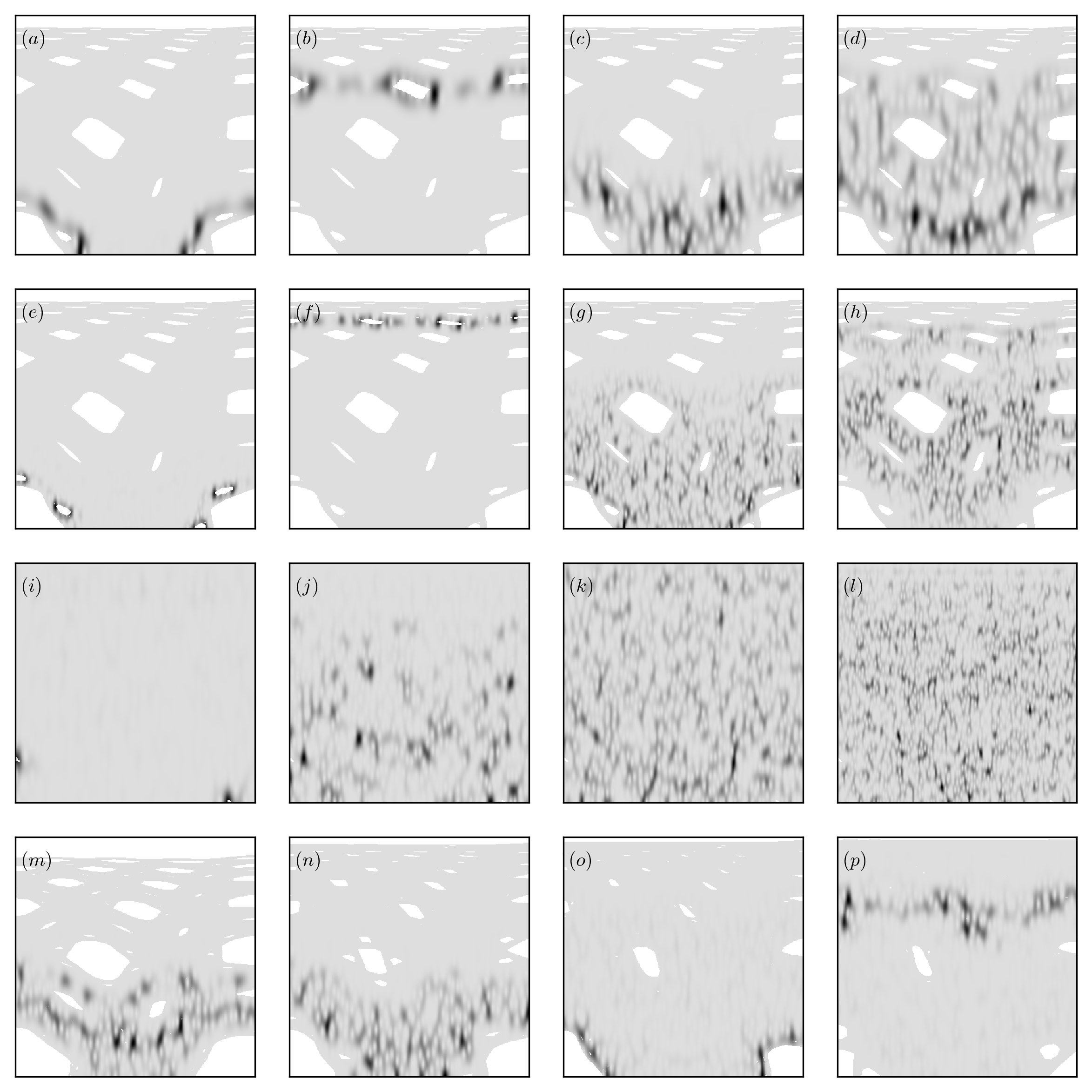
At large (almost ergodic case) and fixed , we have small and according to Eq.(23) , we observe mainly ergodic eigenstates, in agreement with the quantum ergodic theorem Shnirelman 1974, that is fully extended states, exemplified in (k,l). Nevertheless, there are some exceptions, asymptotically of measure zero, where we observe partial localization, as shown in (j). Also, some Poincaré-Husimi functions can be associated with small stability islands around a stable classical orbit exempliifed by (i). Moreover, there can be strongly localized states corresponding to the scaring around and along an unstable periodic orbit in the chaotic sea. More precisely, the area of scars of eigenfunctions goes to zero, and the relative number of scarred states goes to zero as or Heller 1984.
As we decrease and , thereby increasing , the degree of localization increases, thus is decreasing as shown in (a-h). At other values of of strongly pronounced mixed-type phase space we see localized states exemplified in (m-p).
IV The distributions of the localization measures A
In this section we present the central results of this paper, namely the distribution functions of the localization measures . It is found, according to our expectation, that in the almost ergodic case with large such as e.g. , we find that each distribution can be very well characterized and described by the so-called beta distribution
| (26) |
where is the upper limit of the interval on which is defined, and the two exponents and are positive real numbers, while is the normalization constant such that , i.e.
| (27) |
where is the beta function. We shall also use the cumulative distribution defined as
| (28) |
Thus we have
| (29) |
and for the second moment
| (30) |
and therefore for the standard deviation (21),
| (31) |
such that asymptotically when . Whenever we compare from different , we have divided by the relative fraction of the chaotic component in the classical phase space, denoted by , as computed and listed in the table of Ref. Č. Lozej and Robnik 2018a. In the figures 5, 6, 7, 8 we show a selection of typical distributions . In all cases for we have chosen the empirically best value . By we denote the mean value of intervals on which we calculate the 2000 successive eigenstates, from which we extract the chaotic ones, by choosing an appropriate value of , always , in order to make sure that we collect chaotic states. In addition, it should be noted that losing a few chaotic states, which can happen, does not affect the result for in any significant way. It should be noted that the statistical significance is very high, which has been carefully checked by using a (factor 2) smaller number of objects in almost all histograms, as well as by changing the size of the boxes.
The limiting case in Eqs.(29,31) comprising the fully extended states in the limit shows that the distribution tends to the Dirac delta function peaked at , thus and , in agreement with Shnirelman’s theorem Shnirelman 1974.
The Fig. 5 clearly shows that the fit by the beta distribution (26) is excellent in case of , typical for the ergodic regimes with , as observed also in the stadium in Ref. Batistić et al. 2019. The qualitative trend from strong localization to weaker localization or even complete extendedness (ergodicity) with increasing is clearly visible.
In the Fig. 6 we show the distribution for and several values of the shape parameter . Here is normalized by dividing it with . The behaviour that we see is physically very interesting and statistically significant, as we checked carefully, but is not universal, as it depends on the structure of the chaotic component in the classical phase space and on the size and intensity of the stickiness regions. Each stickiness region is expected to support a local maximum in , although this phenomenon is more strongly exhibited in the lemon billiards Č. Lozej et al. 2019. Only at large , when , we see the approach to the beta distribution characteristic of the ergodic regime without stickiness on the underlying chaotic region, exemplified by (j-l), where decreases towards the limit .
We should stress that there is of course some arbitrarines in defining , so long as we do not have a theoretical prediction for its value. So far we have taken , but nevertheless tried also the choice of being the largest member in each histogram, and found no significant qualitative changes, but only minor quantitative differences. In both cases and are not unique functions of , while and might be unique functions of as demonstrated in Figs. 2 and 3, and approximated by a fit in Eq. (25).
V Implications of localization for the spectral statistics of chaotic eigenstates
To get a good estimate of we need many more levels (eigenstates) than in calculating . The parameter was computed for 18 different values of the parameter as given in the Table I, and for 12 intervals in space: where and . This is values of altogether. More than energy levels were computed for each . The size of the intervals in was chosen to be maximal and such that the BRB (Berry-Robnik-Brody) distribution gives a good fit to the level spacing distributions of the levels in the intervals, meaning that is well defined.
For each an associated localization measure was computed on a sample of consecutive chaotic levels around , which is a mean value of on the interval . First, the separation of eigenstates, regular and chaotic, has been done, using , and then the chaotic eigenstates have been studied. Moreover, the obtained distribution functions were calculated for 18 values of and 9 to 12 values of , and some selection of them is presented and discussed in the previous section IV.
The dependence of on , now revised and slightly different than obtained in Batistić and Robnik 2013b, where only one value of was used, is shown in Fig. 9. We show two versions of this plot, one with the classical criterion for (for the BRB distribution), and the other one using the quantum criterion for , when determining by fitting the level spacing distribution with the BRB distribution. The two plots are quite similar, which is satisfactory.
This relation is similar to the case of the quantum kicked rotator Izrailev 1990; Manos and Robnik 2013; Batistić et al. 2013 and the stadium. In both cases the scattering of points around the mean linear behaviour is significant, and it is related to the fact that the localization measure of eigenstates has some distribution , as observed and discussed in Ref. Manos and Robnik 2015 for the quantum kicked rotator, and discussed for the stadium billiard in the Refs. Batistić et al. 2018; Batistić et al. 2019.
There is still a great lack in theoretical understanding of the physical origin of this phenomenon, even in the case of (the long standing research on) the quantum kicked rotator, except for the intuitive idea, that energy spectral properties should be only a function of the degree of localization, because the localization gradually decouples the energy eigenstates and levels, switching the linear level repulsion (extendedness) to a power law level repulsion with exponent (localization). The full physical explanation is open for the future.
As shown in Fig. 10, using the classical criterion for for the fitting BRB distribution, the functional dependence of is always the rational function
| (32) |
only the coefficient depends on the definition of and . For the parameter values we get and .
Similarly, we find for the quantum criterion almost the same results, with no visible differences (not shown).
VI Conclusions and discussion
In this paper we have studied the structural and statistical properties of the eigenstates and their Poincaré-Husimi functions, and of the energy spectra, of a mixed-type billiard Robnik 1983; Robnik 1984, in correspondence with its classical dynamics. The governing control parameter is , where is the Heisenberg time and the classical transport time, as in Eq. (5), in the semiclassical regime of sufficiently small effective Planck constant, which is (the wavelength).
Our main conclusions are as follows: (a) We have confirmed that the normalized inverse participation ratio and the information entropy measure are linearly related and thus equivalent, in agreement with the recent result in the stadium billiard Batistić et al. 2019, which we believe is a general result, not specific of the used model systems. (b) We have calculated the Poincaré-Husimi functions of all eigenstates for 18 different values of the shape parameter and 9 to 12 values of the starting , in each case 2000 eigenstates of even parity. We have shown a selection of typical Poincaré-Husimi functions. (c) Then we have separated the regular and chaotic eigenstates, and verified that the chaotic states are localized to the various degree, and calculated the corresponding localization measure for all of them. (d) We have looked at the distribution functions and (histograms and cumulative distributions), and found that in the regime of uniform chaos (no significant stickiness regions in the classical phase space) they are perfectly well described by the beta distribution, which in the limit of approaches the Dirac delta distribution . This behaviour is the same as in the stadium billiard. (e) In the regime of existing pronounced stickiness regions in the classical phase space, is not universal and can have several maxima (usually it is bimodal), where each minor maximum might be qualitatively attributed to a stickiness region. This phenomenon is under investigation in the lemon billiards Č. Lozej et al. 2019. (f) We have explored the mean value as a function of , which is approximately a rational function, while the standard deviation of , denoted by , as a function of , exhibits strong fluctuations but nevertheless displays a similar structure as in the stadium billiard. (g) The level spacing distribution of localized chaotic eigenstates displays the Brody distribution, where the level repulsion exponent goes from for the strongest localization (Poissonian distribution) to for complete delocalization (ergodicity and GOE). It is a function of , but slightly different from the result in Ref. Batistić and Robnik 2013b, where only one value of has been used. It is closer to the linear relationship, which has been observed in the quantum kicked rotator and in the stadium billiard, but it also depends slightly on the criterion for choosing in determining . It must be emphasized that the transition from strong localization to ergodicity as a function of is a rather smooth one, not a discrete jump, as it takes place over an interval of more than factor in , which is the same behaviour as in the stadium billiard.
We believe that most of our results are quite general, typical for the mixed-type Hamiltonian systems, and where a comparison is applicable, they agree with the previous results on the stadium billiard Batistić et al. 2018; Batistić et al. 2019. Similar extensive analysis is being performed for the lemon billiard Č. Lozej 2019; Č. Lozej et al. 2019, introduced in Ref. Heller and Tomsovic 1993 and studied in Refs. Lopac et al. 1999; Lopac et al. 2001; Makino et al. 2001; Bunimovich et al. 2019, whose classical phase space has been very recently extensively explored by Lozej Č. Lozej 2019. The major open theoretical question is to derive the existence of dynamical localization in chaotic eigenstates, and to calculate the corresponding , and also the level repulsion exponent which governs the level spacing distribution, the underlying distribution being close to the Brody distribution. This problem is not yet solved even for the quantum kicked rotator Izrailev 1990. Further theoretical work is in progress. We expect similar results in the smooth Hamiltonian systems of the mixed-type, such as e.g. the hydrogen atom in strong magnetic field Robnik 1981; Robnik 1982; Hasegawa et al. 1989; Wintgen and Friedrich 1989; Ruder et al. 1994 and the Dicke model Dicke 1954; Furuya et al. 1998; Bastarrachea-Magnani et al. 2015, as well as in experiments such as the microwave resonators introduced and performed by Stöckmann since 1990 Stöckmann 1999.
VII Acknowledgement
This work was supported by the Slovenian Research Agency (ARRS) under the grant J1-9112.
References
- Stöckmann (1999) H.-J. Stöckmann, Quantum Chaos - An Introduction (Cambridge: Cambridge University Press, 1999).
- Haake (2001) F. Haake, Quantum Signatures of Chaos (Berlin: Springer, 2001).
- Robnik (2016) M. Robnik, Eur. Phys. J. Special Topics 225, 959 (2016).
- Wigner (1932) E. Wigner, Phys. Rev. 40, 749 (1932).
- Husimi (1940) K. Husimi, Proc. Phys. Math. Soc. Jpn. 22, 264 (1940).
- Percival (1973) I. C. Percival, J. Phys B: At. Mol. Phys. 6, L229 (1973).
- Robnik (1998) M. Robnik, Nonl. Phen. in Compl. Syst. (Minsk) 1, 1 (1998).
- Berry (1977) M. V. Berry, J. Phys. A: Math. Gen. 12, 2083 (1977).
- Shnirelman (1974) B. Shnirelman, Uspekhi Matem. Nauk 29, 181 (1974).
- Voros (1979) A. Voros, Lect. Notes Phys. 93, 326 (1979).
- Veble et al. (1999) G. Veble, M. Robnik, and J. Liu, J. Phys. A: Math. Theor. 32, 6423 (1999).
- Bohigas et al. (1984) O. Bohigas, M. J. Giannoni, and C. Schmit, Phys. Rev. Lett. 52, 1 (1984).
- Casati et al. (1980) G. Casati, F. Valz-Gris, and I. Guarneri, Lett. Nuovo Cimento 28, 279 (1980).
- Berry (1985) M. V. Berry, Proc. Roy. Soc. Lond. A 400, 229 (1985).
- Sieber and Richter (2001) M. Sieber and K. Richter, Phys. Scr. T90, 128 (2001).
- Müller et al. (2004) S. Müller, S. Heusler, P. Braun, F. Haake, and A. Altland, Phys. Rev. Lett. 93, 014103 (2004).
- Heusler et al. (2004) S. Heusler, S. Müller, P. Braun, and F. Haake, J. Phys.A: Math. Gen. 37, L31 (2004).
- Müller et al. (2005) S. Müller, S. Heusler, P. Braun, F. Haake, and A. Altland, Phys. Rev. E 72, 046207 (2005).
- Müller et al. (2009) S. Müller, S. Heusler, A. Altland, P. Braun, and F. Haake, New J. of Phys. 11, 103025 (2009).
- Gutzwiller (1967) M. C. Gutzwiller, J. Math. Phys. 8, 1979 (1967).
- Gutzwiller (1969) M. C. Gutzwiller, J. Math. Phys. 10, 1004 (1969).
- Gutzwiller (1970) M. C. Gutzwiller, J. Math. Phys. 11, 1791 (1970).
- Gutzwiller (1971) M. C. Gutzwiller, J. Math. Phys. 12, 1791 (1971).
- Gutzwiller (1980) M. C. Gutzwiller, Phys. Rev. Lett. 45, 150 (1980).
- Berry and Robnik (1984) M. V. Berry and M. Robnik, J. Phys. A: Math. Gen. 17, 2413 (1984).
- Prosen and Robnik (1999) T. Prosen and M. Robnik, J. Phys. A: Math. Gen. 32, 1863 (1999).
- Chirikov et al. (1981) B. V. Chirikov, F. M. Izrailev, and D. L. Shepelyansky, Sov. Sci. Rev. C 2, 209 (1981).
- Casati et al. (1979) G. Casati, B. V. Chirikov, F. M. Izrailev, and J. Ford, Lecture Notes in Physics 93, 334 (1979).
- Izrailev (1986) F. M. Izrailev, Phys. Rev. Lett. 56, 541 (1986).
- Izrailev (1987) F. M. Izrailev, Phys. Lett. A 125, 250 (1987).
- Izrailev (1988) F. M. Izrailev, Phys. Lett. A 134, 13 (1988).
- Izrailev (1989) F. M. Izrailev, J. Phys. A: Math. Gen. 22, 865 (1989).
- Izrailev (1990) F. M. Izrailev, Phys. Rep. 196, 299 (1990).
- Borgonovi et al. (1996) F. Borgonovi, G. Casati, and B. Li, Phys. Rev. Lett. 77, 4744 (1996).
- Bunimovich (1979) L. Bunimovich, Commun. Math. Phys. 65, 295 (1979).
- Prosen (2000) T. Prosen, in Proc. of the Int. School in Phys. ”Enrico Fermi”, Course CXLIII, Eds. G. Casati and U. Smilansky (Amsterdam: IOS Press, 2000).
- Batistić and Robnik (2010) B. Batistić and M. Robnik, J. Phys. A: Math. Theor. 43, 215101 (2010).
- Batistić and Robnik (2013a) B. Batistić and M. Robnik, Phys. Rev. E 88, 052913 (2013a).
- Batistić and Robnik (2013b) B. Batistić and M. Robnik, J. Phys. A: Math. Theor. 46, 315102 (2013b).
- Batistić et al. (2019) B. Batistić, Č. Lozej, and M. Robnik, Phys. Rev. E (submitted) (2019).
- Brody (1973) T. A. Brody, Lett. Nuovo Cimento 7, 482 (1973).
- Brody et al. (1981) T. A. Brody, J. Flores, J. B. French, P. A. Mello, A. Pandey, and S. S. M. Wong, Rev. Mod. Phys. 53, 385 (1981).
- Manos and Robnik (2013) T. Manos and M. Robnik, Phys. Rev. E 87, 062905 (2013).
- Batistić et al. (2013) B. Batistić, T. Manos, and M. Robnik, EPL 102, 50008 (2013).
- Robnik (1983) M. Robnik, J. Phys. A: Math. Gen. 16, 3971 (1983).
- Robnik (1984) M. Robnik, J. Phys. A: Math. Gen. 17, 1049 (1984).
- Č. Lozej and Robnik (2018a) Č. Lozej and M. Robnik, Phys. Rev. E 98, 022220 (2018a).
- Č. Lozej and Robnik (2018b) Č. Lozej and M. Robnik, Phys. Rev. E 97, 012206 (2018b).
- Batistić et al. (2018) B. Batistić, Č. Lozej, and M. Robnik, Nonlinear Phenomena in Complex Systems (Minsk) 21, 225 (2018).
- Markarian (1993) R. Markarian, Nonlinearity 6, 819 (1993).
- Č. Lozej (2019) Č. Lozej, Phys. Rev. E (to be submitted) (2019).
- Berry (1981) M. V. Berry, Eur. J. Phys. 2, 91 (1981).
- Tualle and Voros (1995) J. Tualle and A. Voros, Chaos Solitons Fractals 5, 1085 (1995).
- Bäcker et al. (2004) A. Bäcker, S. Fürstberger, and R. Schubert, Phys. Rev. E 70, 036204 (2004).
- Vergini and Saraceno (1995) E. Vergini and M. Saraceno, Phys. Rev. E 52, 2204 (1995).
- Heller (1984) E. J. Heller, Phys. Rev. Lett. 53, 1515 (1984).
- Č. Lozej et al. (2019) Č. Lozej, D. Lukman, and M. Robnik, Phys. Rev. E (to be submitted) (2019).
- Manos and Robnik (2015) T. Manos and M. Robnik, Phys. Rev. E 91, 042904 (2015).
- Heller and Tomsovic (1993) E. J. Heller and S. Tomsovic, Phys. Today 46, 38 (1993).
- Lopac et al. (1999) V. Lopac, I. Mrkonjic, and D. Radic, Phys. Rev. E 59, 303 (1999).
- Lopac et al. (2001) V. Lopac, I. Mrkonjic, and D. Radic, Phys. Rev. E 64, 016214 (2001).
- Makino et al. (2001) H. Makino, T. Harazama, and Y. Aizawa, Phys. Rev. E 63, 056203 (2001).
- Bunimovich et al. (2019) L. A. Bunimovich, G. Casati, T. Prosen, and G. Vidmar, Experimental Mathematics 1, 10 (2019).
- Robnik (1981) M. Robnik, J. Phys. A: Math. Gen. 14, 3195 (1981).
- Robnik (1982) M. Robnik, J. Phys. Colloque C2 43, 29 (1982).
- Hasegawa et al. (1989) H. Hasegawa, M. Robnik, and G. Wunner, Prog. Theor. Phys. Suppl. (Kyoto) 98, 198 (1989).
- Wintgen and Friedrich (1989) D. Wintgen and H. Friedrich, Phys. Rep. 183, 38 (1989).
- Ruder et al. (1994) H. Ruder, G. Wunner, H. Herold, and F. Geyer, Atoms in Strong Magnetic Fields (Heidelberg: Springer, 1994).
- Dicke (1954) R. H. Dicke, Phys. Rev. 93, 99 (1954).
- Furuya et al. (1998) K. Furuya, M. C. Nemes, and G. Q. Pellegrino, Phys. Rev. Lett. 80, 5524 (1998).
- Bastarrachea-Magnani et al. (2015) M. A. Bastarrachea-Magnani, B. L. del Carpio, S. Lerma-Hernandez, and J. G. Hirsch, Phys. Scr. 90, 068015 (2015).