Swampland Conditions for Higher Derivative Couplings
from CFT
Sandipan Kundu
Department of Physics and Astronomy,
Johns Hopkins University,
Baltimore, Maryland, USA
kundu@jhu.edu
There are effective field theories that cannot be embedded in any UV complete theory. We consider scalar effective field theories, with and without dynamical gravity, in -dimensional anti-de Sitter (AdS) spacetime with large radius and derive precise bounds (analytically) on the coupling constants of higher derivative interactions by only requiring that the dual CFT obeys the standard conformal bootstrap axioms. In particular, we show that all such coupling constants, for even , must satisfy positivity, monotonicity, and log-convexity conditions in the absence of dynamical gravity. Inclusion of gravity only affects constraints involving the interaction which now can have a negative coupling constant. Our CFT setup is a Lorentzian four-point correlator in the Regge limit. We also utilize this setup to derive constraints on effective field theories of multiple scalars. We argue that similar analysis should impose nontrivial constraints on the graviton four-point scattering amplitude in AdS.
1 Introduction
By now it is well-known that not all effective field theories (EFTs) can be UV completed. One famous example is the EFT of a massless scalar with higher derivative interaction
| (1.1) |
which does not admit a UV completion for [1]. Conceptually, this represents a substantial departure from our traditional understanding of Wilsonian EFTs. In fact, this remarkable result led to the proof of the 4D -theorem establishing irreversibility of unitary renormalization group flows between conformal fixed points [2]. More generally this constraint is related to the idea of “swampland” of EFTs that cannot be obtained as a low energy approximation of a consistent theory of quantum gravity (oftentimes string theory) [3, 4, 5, 6, 7, 8].
The constraint on the EFT (1.1) is not actually an accident, but part of a general feature of low energy EFTs with higher derivative interactions. There is a growing body of literature with similar precise bounds on IR couplings of an EFT from UV consistency [9, 10, 11, 12, 13, 14, 15, 16, 17, 18, 19, 20, 21, 22, 23, 24, 25]. All these bounds have one thing in common that they do not depend on the details of the UV completion. However, these types of bounds are generally derived under the assumption that the scattering amplitude obeys (i) analyticity (in the usual regime), (ii) partial wave unitarity, (iii) crossing symmetry, and (iv) Regge boundedness conditions even in the UV. Such S-matrix based arguments can be unsatisfying since some of these assumptions (even though well-motivated) have not yet been rigorously established.11 1 In recent years, significant progress has been made both in analytical and numerical approaches to the S-matrix bootstrap [26, 27, 28, 29, 30, 31, 32, 33, 34, 35, 36, 37, 38, 39, 40, 41, 42, 43, 44, 45, 46].
Another technical challenge of these EFT arguments is to incorporate dynamical gravity mainly because of the graviton pole in the scattering amplitude. Recently, an elegant framework has been introduced in [47] that bypasses this problem by studying scattering amplitudes at finite impact parameter (see [48] for related discussions). Under the same assumptions about the scattering amplitude, this framework leads to non-trivial and rigorous two sided bounds on coupling constants of higher derivative interactions in dimensions. The analysis necessarily requires that the scattering amplitude for large (at fixed ). However, it is unclear whether this Regge boundedness condition is valid in the presence of dynamical gravity.22 2 Note that the Froissart bound [49, 50, 51] does not hold without a mass gap in the theory. Hence, the Regge boundedness condition is subtle whenever there are massless states in the theory, even in the absence of gravity. For example, the same issue persists even for the 4-point scattering amplitude of the dilaton that led to the proof of the 4D -theorem in [2]. However, in that case, the Regge boundedness follows from conformal invariance of the UV fixed point [52, 53]. On the other hand, the same argument for the 4-point dilaton amplitude in 6D imposes a weaker condition [54, 55]. Nevertheless, these bounds provide compelling evidence in favor of the expectation that all higher derivative interactions must have order one coupling constants in the units of the UV cut-off scale. The main motivation of this paper is to derive similar bounds on EFTs in anti-de Sitter (AdS) spacetime where such loopholes can be avoided.
In this paper, we will address a closely related question: what scalar EFTs in AdSD cannot be embedded into a UV theory that is dual to a CFTD-1 obeying the usual CFT axioms? We will provide a partial answer to this question by leveraging the huge advancement in constraining the space of consistent CFTs from well-established conformal bootstrap axioms (for a review see [56]). The main logic of our argument parallels recent developments in constraining EFTs in AdS (with or without dynamical gravity) from rigorous analysis in the dual CFT [57, 58, 59, 60, 26, 61, 62, 63, 29, 64, 65, 66, 67, 32, 68, 69, 70, 71, 72, 73, 74]. For example, the sign constraint on the coupling in the EFT (1.1) can be derived in AdS from the conformal bootstrap [58].
The main advantage of our AdS argument is that the bounds follow directly from the conformal bootstrap axioms which are, both conceptually and technically, well-understood, at least at the level of four-point correlators. We will derive the constraint (with and without dynamical gravity) as a special case of an infinite set of similar constraints on higher derivative interactions of the form from a simple CFT setup.
We consider a scalar EFT in AdSD with an effective action33 3 We are ignoring , , , and all other higher derivative interactions that cannot be written as since these interactions, as well as presence of other low spin fields, will not affect the final bounds. However, these interactions can sometimes create obstruction to a flat space limit, especially at low spacetime dimensions. We will discuss this in section 4.3.
| (1.2) | ||||
where, is the Einstein-Hilbert action with a negative cosmological constant and is the mass-scale of new physics. We allow for the possibility that the scalar field has a mass . First, let us explain our convention. We have defined a positive coupling constant which has the dimension . The coupling constants are dimensionless and normalized by introducing (dimensionless and known) positive numerical factors .44 4 The numerical factor is defined in (4.17) as ratios of -functions. Note that . Moreover, in the large AdS radius limit with finite and non-zero , this factor for all finite . For large AdS radius, the numerical factor is non-trivial (i.e., ) only in the massless limit (or for ). The choice of this particular normalization makes the final bounds rather simple. Moreover, without loss of generality, we will assume that is order one, however, to begin with we do not assume that the other coupling constants are order one as well. Our goal is to derive necessary conditions (analytically) for the tree level EFT (1.2) to have a UV completion.55 5 We assume that the EFT (1.2) is weakly coupled such that (if non-zero) and are small and of the same order in the units of the cut-off scale . In particular, we will impose precise constraints on coupling constants, irrespective of the details of the UV physics, from the requirement that the dual CFT satisfies the bootstrap axioms.
There are non-trivial constraints on the EFT (1.2) even when gravity is non-dynamical . So, first we focus on this simpler case. The EFT (1.2) in AdS with large radius enjoys a dual CFT description in spacetime dimensions. Specifically, it was shown by [75] and subsequent authors [76, 77, 78, 79, 80, 81, 82, 83, 84, 85, 86, 87], that the scalar EFTs in AdSD of the form (1.2) are in one-to-one correspondence with perturbative solutions of crossing symmetry in CFTD-1. This interacting dual CFT has a scalar primary operator which is dual to the AdS field with dimension given by . Since there is no dynamical gravity, the stress tensor of the dual CFT must decouple from the low energy spectrum. This implies that we are in the limit of large central charge with fixed (but large).66 6 The central charge is the overall coefficient of the CFT stress tensor two-point function. Of course, the dual CFT should be thought of as an “effective” CFT which is embedded in some bigger CFT satisfying the usual CFT axioms. We utilize this dual description to study CFT Regge correlators associated with the EFT (1.2). At the leading order in , these CFT Regge correlators grow in a very specific way within the regime of validity of the EFT (1.2). In fact, this type of Regge growth is known to be highly constrained by the argument of [88] (see section 6). In this paper, we revisit these bounds on the Regge growth of CFT correlators and show that they impose precise constraints on the EFT (1.2). In particular, in the limit of large we conclude that the coupling constants , irrespective of the rest of the theory, must obey the following conditions for the EFT (1.2) (with ) to be embedded into a UV theory that is dual to a CFT obeying the CFT axioms:77 7 All bounds obtained in this paper are valid in spacetime dimensions . We also expect that our analysis is valid even for as long as and the field has shift symmetry or symmetry.
- •
Positivity– For all even
(1.3) - •
Monotonicity– as a function of even decreases monotonically88 8 It should be noted that this condition, unlike other two conditions, depends on our exact definition of the cut-off scale . For an arbitrary definition of , there must always exist a rescaling with order one which makes the EFT consistent with the condition (1.4).
(1.4) for all even .
- •
Log-Convexity– , for even , satisfies a global log-convexity condition and hence for any even , , and
(1.5)
We emphasize that these constraints follow directly from analyticity, positivity, and crossing symmetry of CFT four-point correlators – properties that are contained in the conformal bootstrap axioms. The above conditions, among other things, imply that all higher derivative interactions with even must have order one coupling constants in the units of the UV cut-off scale . However, we believe that (1.3)-(1.5) are necessary conditions but they are far from being sufficient. For example, it is expected that similar bounds exist even for odd . Whereas, our setup does not impose any restriction on the odd couplings other than all couplings in AdS, even or odd, with must vanish when .99 9 This can be alternatively stated as with . This condition is more subtle in the exact flat space limit, as we explain later. In flat space does not necessarily requires for odd . For an example see [55].
Of course, the next key step is to include dynamical gravity (). In our setup, the inclusion of gravity is a rather trivial generalization. Now the central charge of the dual CFT is large but finite. The bulk graviton contributes only to the leading growing term of the Regge correlator of the dual CFT. This immediately implies that the constraints (1.3)-(1.5) remain unchanged for all even . On the other hand, all conditions involving now receive corrections from gravity. For example, gravity allows for the interaction to have a negative coupling constant
| (1.6) |
where is a positive order one numerical factor given in appendix F. It is however unclear how to extract a precise bound from (1.6) in the flat space limit. The AdS bound (1.6), as we will explain, suggests that in the flat space limit , where is some small positive number. This is certainly consistent with the results of [47], however, we do not have a precise definition of . Nevertheless, this raises an interesting conceptual question of whether, and in what sense, the 4D -theorem is valid in the presence of dynamical gravity.
Finally, we will generalize our analysis for EFTs of multiple scalar fields in AdS. The main motivation for this generalization is to demonstrate that there are other tools available when we go beyond a single scalar field. For example, the same CFT consistency conditions of [88] now also impose two-sided bounds on odd higher derivative interactions involving multiple fields (see [25] for similar bounds on flat space multi-field EFTs). Furthermore, for multiple fields there are interference effects that are also constrained by the CFT axioms leading to an infinite set of non-linear bounds among various higher derivative coupling constants.1010 10 Note that the same interference effects were utilized in [72] to derive non-linear bounds on the dilaton-axion effective action associated with 4D RG flows with global symmetry breaking. These additional tools will certainly be useful for bounding the four-graviton scattering amplitude in AdS by using the dual CFT description.
Our CFT setup, from the dual gravity perspective, is probing local high energy scattering deep in the bulk. Since the local high energy scattering is insensitive to the spacetime curvature, on physical grounds we expect that AdS bounds obtained in this paper persist even in the flat space limit (other than the caveat mentioned after equation (1.6)). Indeed, we checked that weakly coupled string amplitudes satisfy all the conditions derived in this paper. However, there is one obvious but important issue that we must address. Any strict AdS inequality must be regarded as in the flat space limit since the case can no longer be ruled out due to finite curvature effects.
An important feature of our AdS bounds is that they differ significantly for massive and massless scalars, especially when we take the flat space limit. In particular, when we take the large limit (with fixed ), our bounds agree completely with the ones obtained from the flat space dispersive sum-rules under the same set of assumptions about the four-point amplitude as mentioned in the beginning.1111 11 This is true even when we take after taking the large radius limit. See section 5. On the other hand, when we take first and then , two sets of bounds differ significantly. This perhaps indicates that the Regge boundedness condition of the flat space amplitude can break down in the presence of massless states (see section 5).
At this stage, one may wish to compare our bounds with the flat space bounds of [47]. Indeed, there is some overlap between these two sets of bounds. Of course, from our CFT setup, it is not immediately clear how to obtain any constraints on odd coupling constants for a single scalar field. Such bounds will perhaps require a more sophisticated CFT analysis. Nevertheless, we observe that our constraints, in the flat space limit, are consistent with the bounds of [47].
We have analyzed the EFT (1.2) at tree level. We note that the CFT consistency conditions of [88] that we have utilized in this paper apply even when we include corrections from EFT loops. In fact, the CFT consistency conditions of [88] (see section 6) hold even for arbitrary external CFT operators with or without spins (and not necessarily local or primary). So, it is a straightforward exercise to extend our analysis to derive bounds on the graviton four-point scattering amplitude in AdS by studying Regge correlators of the stress tensor operator in the dual CFT. It would be interesting to compare such bounds with similar classical bounds of [89] from “Classical Regge Growth” (CRG) conjecture and EFT bounds of [90, 91] from unitarity and crossing. We will have to leave this question for the future.
The rest of the paper is organized as follows. In section 2 we begin by explaining our general setup. In section 3 we review the bounds of [88] on certain CFT Regge correlators and explain how they follow from the conformal bootstrap axioms. We use this CFT constraints in section 4 to derive bounds (1.3)-(1.5) on the scalar EFT in AdS without dynamical gravity. Then in section 5 we discuss some implications of these constraints for massless external scalars in the flat space limit. Section 6 studies the consequences of the inclusion of gravity. In section 7 we extend our analysis to impose bounds on the EFT of two scalar fields. Section 8 contains our conclusions and final comments. Some additional aspects of our analysis are included in several appendices. In particular, in appendix A we demonstrate how Rindler positivity in CFT follows from unitarity and crossing symmetry.
2 Scalar EFT in AdS
We consider an EFT of a single massless or massive scalar field in AdS with higher derivative interactions. We start with the following low energy effective action with four-point interactions
| (2.1) |
where, and are coupling constants.1212 12 Note that at the tree level the term can be removed by using the equation of motion. So, we will ignore the interaction completely. The AdS radius is large but finite. Our goal is to derive constraints on the coefficients . In the process, the form of the effective action (1.2) will emerge automatically. Note that different higher derivative interactions, in general, can be suppressed by different scales. However, we will assume that all interactions are suppressed by some small coupling :
| (2.2) |
We intend to impose constraint on the weakly coupled effective theory and hence we work in the leading order in .1313 13 One can think of as the analog of the string coupling in string theory. Similarly, the cut-off scale in the effective action (1.2) can be regarded as the string scale. This will be implemented by keeping only tree level processes.
It should be noted that there are higher derivative 4- interactions (with 12 or more derivatives) that cannot be written as even when we apply the equation of motion. However, these other higher-derivative interactions are not bounded by the argument of this paper, provided is non-zero. Hence, we ignore these other higher derivative 4- interactions since they will not affect any of the bounds obtained in this paper. We will discuss this again in section 4.4 in detail.
2.1 Dual CFT
We will impose constraints on this action from the consistency of the dual CFTd, where . The AdS theory (2) is dual to an interacting CFT in -dimensions. The bulk field is dual to a scalar primary operator with dimension . The two-point function is completely fixed by conformal invariance1414 14 For a review see appendix C.
| (2.3) |
Of course, the graviton is dual to the CFT stress tensor . The EFT (2) is a well behaved theory at energies below the cut-off scale . Our goal is to impose constraints on the coupling constants by requiring that the EFT is the low energy description of a UV complete theory. Equivalently, in the CFT side we will assume that the dual CFT is well behaved. Next, we discuss exactly what we mean by a well behaved CFT.
2.2 CFT Axioms
We make the assumption that the dual CFT obeys the Euclidean bootstrap axioms. In particular, we only make use of the following three properties:
- (i)
OPE Unitarity– All OPE coefficients of real operators are real.
- (ii)
Crossing Symmetry– CFT four-point correlators are crossing symmetric.
- (iii)
Analyticity– Lorentzian CFT four-point correlators are analytic in the usual domain (see figure 3).
These CFT properties are well-established and they imply rigorous non-perturbative constraints on certain Regge correlators as derived in [88]. We will use these constraints to derive precise bounds on the higher-derivative couplings of the EFT (2).
3 A Review of the Bounds on CFT Regge Correlators
In this section we review the bounds of [88] on CFT Regge correlators for scalar external operators. Points in CFTd are denoted as follows:
| (3.1) |
where, are lightcone coordinates. We study the Lorentzian CFT correlator1515 15 The Hermitian conjugatation in (3.2) acts only on operators, not on coordinates.
| (3.2) |
of two arbitrary CFT scalar operators, where operators inside the correlator are ordered as written. All the points are restricted to be on a 2d subspace:
| (3.3) |
with and , as shown in figure 2. The operator ordering in (3.2) is important since some of the operators, as shown in the figure 2, are timelike separated. This Lorentzian correlator can be obtained from the Euclidean correlator by analytically continuing along the path shown in figure 3.
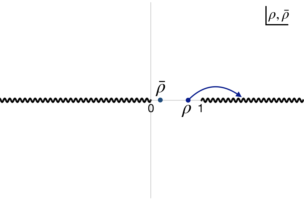
For later convenience, we parametrize
| (3.4) |
with and hence . The CFT Regge limit can be reached by taking
| (3.5) |
of the correlator . The Regge correlator , as a function of complex , is analytic near (for ) on the lower-half -plane [92, 93, 88].
3.1 Boundedness of the Regge Correlator
We can define another Lorentzian correlator
| (3.6) |
which is determined by Euclidean OPE and hence in the limit (3.5)
| (3.7) |
where dots represent terms that are suppressed by positive powers of . The Regge correlator is bounded by the “Euclidean” correlator . In particular, for real with OPE unitarity and crossing symmetry imply
| (3.8) |
where, . In the strict Regge limit (3.5), this simplifies to
| (3.9) |
with .
3.2 CFT Constraints
Next, we focus on Regge correlators with a very specific Regge behavior for some range of :
| (3.10) |
up to terms that decay in the Regge limit. The cut-off dictates the regime of validity of the Regge expansion (3.10). Later we will relate to .
The Regge correlator , as a function of complex , is analytic near on the lower-half -plane [92, 88]. Using this analyticity property we can write a CFT dispersion relation for [88]:
| (3.11) |
where . The above relation leads to bounds on for all . Note that the left hand side does not depend on . This implies deviates significantly from 1 only when . This is closely related to the fact that the tree level 4-pt scattering amplitude for the EFT (2) has no imaginary part.
Positivity
The boundedness condition (3.9) immediately implies [88]
| (3.12) |
for . One can worry whether the correction terms in (3.9) can affect the above positivity condition for higher . For the CFT dual to (2), we can always take a limit where is small enough such that these corrections are suppressed.1616 16 At the end of this section we will discuss more about these corrections.
Parametric Separation
Log-Convexity for Even
The Cauchy-Schwarz inequality of integrable functions leads to the log-convexity condition for with even [88]:
| (3.15) |
and .
Boundedness of Odd
There is no sign constraint on with odd . However, the absolute value of for odd is bounded [88]
| (3.16) |
and . This also follows from the positivity condition (3.9) and the Cauchy-Schwarz inequality.
Note that the chaos sign and the growth bounds of [94] are contained in the above consistency conditions. The condition (3.12) is a generalization of the chaos sign bound. Whereas, the condition (3.13) implies that the Regge correlator (3.10) must not grow faster than within the regime of validity .
Finally, let us note that the above constraints hold for arbitrary external operators with or without spins (and not necessarily primary)1717 17 See [88] for details. as long as the Regge correlator has the form (3.10). For such a general case, the positivity of the integrand in (3.11) follows from Rindler positivity.
3.3 Correction Terms and Validity of the CFT Dispersion Relation
All of the above constraints depend on the dispersion relation (3.11). So, it is only natural to ask whether there are corrections to this dispersion relation. In this section, we argue that any such correction terms do not affect the dispersion relation (3.11) since they are always suppressed for CFTs that are dual to some EFT in AdS. Casual readers may skip this subsection.
The first correction comes from the terms of (3.9). Moreover, similar correction terms can be present in the Regge expansion (3.10). So, the leading correction to the dispersion relation (3.11) comes from a term
| (3.17) |
since all terms with negative have integer with imaginary coefficients.1818 18 It is important to note that any correction term with integer (positive or negative) power of and an imaginary coefficient cannot affect the sum-rule (3.11) [88].
First, let us justify the dispersion relation (3.11) for the scenario where operators and are different. In this case, especially for CFTs that are dual to some EFT in AdS, it is easy to see that since CFT operators that are exchanged are either double trace operators or single trace operators with from a bulk three-point interaction.1919 19 Let us recall that we are restricting to the case where all fields have . In particular, the contribution of a correction term (3.17) to the dispersion relation of is given by
| (3.18) |
where the line integrals are evaluated just below the real -axis. Now, note that the leading contribution to , whereas, the leading contribution to comes from scalar three-point couplings: . Therefore, for any non-zero , the correction term is suppressed for
| (3.19) |
On the other hand, the cut-off scales as .2020 20 This can be seen easily from the scaling of individual terms of the expansion (3.10) for the bulk theory (2). In particular, the expansion (3.10) for the Regge correlator of the dual CFT is an expansion in the quantity , as can be seen from (4). The cut-off is controlled by the relative strength of consecutive terms in the expansion (3.10) and hence . Therefore, for large we can always choose such that the correction term is parametrically suppressed for .2121 21 We are also making the mild assumption that is not parametrically small when measured in the units of the mass cut-off scale (for example , as defined in the introduction) associated with the bulk theory (2). If three-point bulk interactions such as are absent, all other corrections (even from the bulk graviton exchange) to the sum-rule are more suppressed. Hence, the dispersive sum-rule for can always be trusted, at least for , for small .
Let us now analyze the relation (3.11) for higher . Note that we can estimate:
| (3.20) |
which implies
| (3.21) |
where we see from (3.20) that and hence the second term can be ignored just like before even for .2222 22 For odd , it is possible that because of cancellations implying that the dispersion relation (3.11) is not reliable. However, in this case all of the CFT bounds for odd are satisfied automatically.
When , there is a loophole in the above argument which we now fix. The disconnected Witten diagrams associated with the 4-pt correlator of the scalar operator of dimension have the leading correction term with order 1 coefficient. However, one can subtract these contributions without affecting any of the bounds on . For example, when of the external scalar operator is an integer, we can replace in the sum-rule (3.11) by , where is the correlator (3.6) for the AdS theory (2) without any interactions. This new sum-rule holds because is analytic on the lower-half plane for integer . Moreover, is positive on the real line up to correction terms that are exactly the same as the above discussion of nonidentical operators. So, we repeat the same argument again to conclude that the modified dispersive sum-rule for is reliable for and integer . This is sufficient for us, since for any fixed , we can always tune such that is an integer. In any case, for non-integer one can still write a more general sum-rule for by subtracting contributions from the identity operator in all channels. The procedure is outlined in appendix B.
4 Constraining Scalar EFT in AdS without Gravity
The main goal of this section is to impose bounds on the EFT (2) from CFT consistency conditions. To that end, we compute contributions of each EFT interactions to the Lorentzian correlator
| (4.1) |
in the Regge limit (3.5), where operator is dual to the scalar field . First, we consider the purely non-gravitational case by setting . The leading contribution to the correlator comes from the disconnected Witten diagrams. The dominant subleading contribution comes from the tree level Witten diagrams that are shown in figure 4.
Before we proceed with the computation, let us review what is already known about the Regge limit. For example, from [75, 95] we know the scaling of the leading Regge contribution of each interaction in (2):
| (4.2) |
for integer . From the scaling behavior (4) it is clear that the Regge correlator (4.1) has the desired expansion (3.10) up to terms that are suppressed by positive powers of . Notice that contributions of for odd are always suppressed in the large limit. Hence, the above scaling behavior implies that we can only impose constraints on interactions for from the CFT consistency conditions of the preceding section.
We observe that the leading contribution to with even comes entirely from the interaction . Contributions from interactions to are all suppressed in the large limit. It is also clear from (4) that with odd are all zero. This simply follows from the fact that is a real scalar operator.
So, it is sufficient for us to consider each interaction separately
| (4.3) |
with being an even integer, where . Note that
| (4.4) |
where dots represent terms with lower number of derivatives after we impose the free equation of motion.
It is more convenient to first compute the Euclidean correlator and then analytically continue to obtain the Regge correlator. So, the on-shell Euclidean action associated with (4.3) is obtained from (C.2)
| (4.5) |
where again dots represent terms with lower number of derivatives that cannot contribute to . This on-shell action can be further simplified by using the bulk-to-boundary propagator (C.5)
| (4.6) |
where the derivatives are taken with respect to the bulk point .2323 23 The coefficient is defined in (2.3). In the above expression, we have utilized the notations of [96]
| (4.7) |
Note that represents points on the AdS boundary. Moreover, the reduced bulk-to-boundary propagator is defined in (D.3) to reduce clutter. The boundary value of the field is given by which acts as the source for the CFTd primary operator in the usual way.
We can now use the identity (D.1) to write in terms of the -function which is defined in (D.1) in the standard way. We notice from equation (D.16) that all -functions decay in the Regge limit . On the other hand, factors for the kinematics (D.2) can grow as . Therefore, terms in that have the largest factors of dominate in the Regge limit (3.5). This greatly simplifies the analysis since we only care about the growing part of the Regge correlator . In particular, the leading Regge contribution from the on-shell action (4) comes from
| (4.8) |
where, dots represent terms that will not contribute to . It is now a straightforward exercise to show that the leading Regge contribution of the interaction (4.3) is
| (4.9) |
where . From the above result, we obtain an expression for for even in the limit of large (with fixed):
| (4.10) |
where, is a positive coefficient independent of
| (4.11) |
and the -function is given by using (D.2):
| (4.12) |
which is positive for . As we mentioned before, all coefficients with odd vanish exactly.
4.1 Bounds
We are now in a position to utilize the CFT constraints from section 3.2 to derive bounds on the EFT (2).
4.1.1 Positivity
First, we impose the condition (3.12). The fact that both and for are positive immediately implies
(4.13)Moreover, saturation of any one of (4.13) necessarily requires that the all of them are saturated. These bounds are consistent with the flat space bound of [1] from analyticity and unitarity of scattering amplitudes. Note that there is no such positivity condition on with odd from the CFT consistency conditions.
4.1.2 Scale suppression of higher derivative interactions
We now impose the condition (3.13). First, let us apply (3.13) to :
| (4.14) |
for all , where we are assuming that the AdS theory is interacting (). First thing we notice that a mass scale is emerging naturally where we have identified
| (4.15) |
This definition of needs some explanation. It is expected that since deviates significantly from 1 when implying a breakdown of (3.10). The exact power in (4.15) follows from the linear relationship between . The order one numerical factor has been chosen such that in certain scenarios has the physical interpretation of the lightest heavy state exchanged.2424 24 We will make this more precise in section 5. Given a UV complete CFT dual and the low energy Regge behavior (3.10), one can compute from the sum-rule (3.11) with . Then (4.15) should be thought of as a precise definition of . The bulk cut-off scale is then given by the relation: . Of course, this definition of is not unique. This definition is analogous to the definition of in [47] and in certain cases these two definitions are exactly equivalent, as we show in section 5.
The strongest bound from (4.14) is obtained for the value of that minimizes the right hand side. One can check that this is achieved in the limit . Therefore, by using results from appendix D.3 we obtain a strict bound:
(4.16)where, is given by
| (4.17) |
with . Of course, the bound (4.16) depends heavily on our definition of (4.15). Notice that is the same coefficient that appears in (1.2).
The bound (4.16) validates our expectation that higher derivative interactions are suppressed by inverse powers of for even . However, CFT consistency conditions of the preceding section do not impose similar constraints on interactions with odd . This perhaps suggests that our bounds are far from being optimal.
Let us make few comments about the coefficient which is a log-convex function of . From (4.17) we find that for any and implying
| (4.18) |
We will derive this relation in flat space by assuming the Regge boundedness condition: for large . In that case, is the mass of the lightest massive state exchanged. This explains the choice (4.15).
Furthermore, note that is non-trivial only in the massless limit . In particular, if we take with fixed , we obtain
| (4.19) |
for all finite . Therefore, for non-zero , all our bounds simplify greatly.
4.1.3 Log-convexity condition
4.1.4 Odd couplings
We still can say few things about the odd couplings. First of all, if the leading contribution to comes from . However, this contribution to changes sign as we tune within the domain for (see appendix E). Hence must vanish exactly. Then the condition (3.13) implies that
(4.21)for even or odd .2525 25 We assume that . For negative mass2, see appendix E for comments. When , the bound on odd couplings are rather weak. The above argument then implies that for odd .
4.2 Final Effective Action
Let us now summarize the results of this section by writing the AdS scalar effective action (2) as follows
| (4.22) |
where is the scale of new physics and the numerical factor is defined in (4.17). The scalar field can have mass but . Note that for any and . For , , in the large limit, differs from 1 only for .2626 26 More generally, in the large limit, with differs from 1 only for and with fixed.
So far gravity is non-dynamical . We have defined a positive coupling constant which has the dimension . The -coefficients are dimensionless, however, to begin with we do not assume that they are . We do assume the theory is weakly coupled and hence analyze the theory at tree level.
The main goal of this paper is to address the question: when can this EFT be UV completed? Or equivalently what are the necessary conditions for this EFT to be embedded into a UV theory that is dual to a CFT with obeying the CFT axioms? In this section, we conclude that the EFT (4.2), with , must have the following properties ():
- (i)
for all even ,
- (ii)
for all even ,
- (iii)
for all even .
The last condition follow directly from the local log-convexity condition (4.20). It should be noted again that the condition (ii) depends on the exact definition of and hence the scale . On the other hand, other two conditions do not depend on the exact definition of the scale . For an arbitrary definition of , the condition (ii) should be thought of in the following way. There must always exist a rescaling , with order one , which makes the EFT consistent with the condition (ii).
It should also be emphasized that (i)-(iii) are necessary conditions but we believe they are far from being sufficient. For example, it is expected that similar bounds exist even for odd .2727 27 Note that the condition (4.21) has been implemented by assuming the EFT has the form (4.2) along with . However, our argument does not impose any restriction on the odd couplings other than .
4.3 Flat Space Limit
We end this section with some discussion on the flat space limit of the EFT (4.2). In this section we restrict to the massless case: . The flat space limit should be taken in the following way:
| (4.23) |
In the massless case
| (4.24) |
increases fast for as we increase . In this limit, the constraints (i)-(iii) lead to bounds on the flat space EFT of a massless scalar. We can compare these flat space bounds with the results from [47] by relating various coupling constants:
| (4.25) |
In particular, in the absence of gravity we obtain
| (4.26) |
Furthermore, with our definition of , we find that the bound (4.18) agrees with the bound obtained in [47].
As we will explain in section 6, all bounds for with remains unaffected even when gravity is dynamical. Furthermore, we obtain a rather interesting inequality by applying (iii):
| (4.27) |
It would be interesting to compare this bound with the analysis of [20]. It is possible to derive an infinite set of such constraints from (iii). Note that constraints involving will only be affected when gravity is turned on. Let us stress that there is a discreet difference between the massless case and the massless limit when we take the flat space limit. We will discuss this in the next section.
Unlike [20, 47], our analysis is insensitive to and interactions of (4.2). However, we still need to pay attention to these interactions. In particular, the coupling constant for the interaction has positive mass dimension for . So, this coupling can lead to large mixing effects in the dual CFT when we take the flat space limit [68]. In particular, when
| (4.28) |
there is a large mixing between the naive generalized free field operator and because of the decay channel . It is unclear whether the flat space bounds are reliable when the mixing effect is large. Nevertheless, we can avoid this issue for by giving the bulk field some symmetry. Or we can take the flat space limit of the AdS theory (2) such that
| (4.29) |
There is one more subtlety that we must address. When the interaction is absent in the AdS EFT (4.2), all the higher derivative interactions must also vanish. However, our analysis does not require this to be true in the exact flat space limit. For example, the coefficient of the interaction can be suppressed by in such a way that the dual CFT is well behaved. Moreover, the EFT can have a interaction which is not suppressed by but fine-tuned such that is still positive. In this scenario, the interaction goes to zero in the flat space limit with a non-vanishing interaction. It has been recently conjectured that such EFTs emerge naturally in the IR from 6D supersymmetric RG flows on to the Higgs branch [55]. So, such RG flows in AdS6 with finite radius are expected to generate a interaction for the dilaton which is suppressed by .
4.4 Other Higher-Derivative Interactions
The observant reader may have noticed that the effective action (4.2) can have other higher derivative 4- interactions. For example, even in flat space there are multiple inequivalent 4- interactions with 12 or more derivatives. In this section, we will argue that these other higher-derivative interactions are not bounded by the argument of this paper (provided is non-zero). So, these other higher derivative 4- interactions will not affect any of the bounds obtained in this paper.
First, let us consider the flat space EFT (massive or massless) with 4- interactions. At the -derivative level, there are exactly two types of interactions:
| (4.30) |
All other possible interactions can be written in the above form by utilizing the free equation of motion and integration by parts. Note that the second term can only be non-zero and indepedent (when we use the equation of motion) for .2828 28 For example, for the second term can be equivalently written as plus terms with 4 or less derivatives.
Now we move on to the AdS case and replace . In AdS, derivatives do not commute in general. So, one may construct several more terms from the second term of (4.30) by choosing different ordering of derivatives. However, different derivative orderings differ only by factors of
| (4.31) |
and hence derivative ordering is not important in the large limit. Let us now figure out the Regge contribution of the second term of (4.30) in AdS. One can easily check that the leading Regge contribution of the second term comes from the on-shell action
| (4.32) |
which grows slower than since . Hence, for even , the leading Regge contribution always comes from the first term of (4.30). Therefore, we conclude that these other higher derivative 4- interactions do not affect any of the bounds obtained in this paper.
5 Flat Space Limit: Massless & Massive Scalars
In this section, we compare bounds from the previous section with bounds obtained by studying flat space scattering amplitudes. We again start with the effective action (2) without dynamical gravity . For simplicity we take the three-point coupling , so that the tree level 4-point scattering amplitude does not have poles at . The forward limit () of the tree level 4-point scattering amplitude associated with the effective action (2) is given by
| (5.1) |
At this point we make four assumptions: (1) the forward amplitude is bounded for large :
| (5.2) |
(2) the amplitude is analytic in the upper-half complex -plane, (3) the amplitude obeys partial-wave unitarity implying for real , (4) the amplitude is crossing symmetric.
These are the key assumptions which allow us to write a dispersive sum-rule for . In particular, repeating the argument of [1], we can write
| (5.3) |
for all even , where is the cut-off scale at which becomes non-zero. The cut-off scale , however, the two scales can be different in general by some order one proportionality constant.
From (5.3), we can also derive a monotonicity and a log-convexity conditions for even :
| (5.4) |
The second inequality can be used to derive a global log-convexity condition (1.5) for even .
Thus, under the above assumptions we showed that the tree level amplitude, in the forward limit, has a polynomial expansion in with coefficients obeying (i) positivity, (ii) monotonicity, and (iii) log-convexity conditions. At first sight, these conditions seem to be stronger than the flat space limit of the AdS conditions (1.3)-(1.5). For the remainder of this section we will address whether, and in what sense, the above bounds are related to the AdS bounds.
5.1 Massive Scalars
An important feature of our AdS bounds is that they differ significantly for massive and massless scalars, especially when we take the flat space limit. First, we consider the massive case , where is the cut-off scale defined in the previous section. We take the flat space limit by , keeping fixed. So, in this limit and hence
| (5.5) |
for all . Therefore, in this case, for all and the AdS conditions (1.3)-(1.5) are identical to conditions (5.3) and (5.4) that were derived from the flat space sum-rule, provided we identify . This provides compelling evidence in favor of the assumptions that were used to derive the sum-rule (5.3) for massive external scalars. Moreover, for massive scalars, as we will explain in the next section, conditions (5.3) and (5.4) remain valid for even even when there is dynamical gravity. This is rather non-trivial since the validity of the Regge boundedness condition (5.2) is not obvious in the presence of the graviton.
5.2 Massless Scalars
The situation is a lot more subtle for massless external scalars. We can start with and then take the large limit. One can also take a massless limit in which we first take the large limit (with fixed ) and then . Clearly, our bounds are different in these two limits. In the latter case, we again obtain (5.5). Hence, conditions (5.3) and (5.4) still hold. For example, in this case (4.27) becomes
| (5.6) |
On the other hand, if we take first, we obtain bounds from section 4.3. In particular, now we have conditions (1.3)-(1.5) with given by (4.24). These bounds are weaker than the conditions (5.3) and (5.4).
Furthermore, the massless limit can also be taken in a more general way: , with fixed. In this case, we again obtain the weaker set of bounds (1.3)-(1.5) with given by (4.17). Therefore, depending on how we take the massless limit (or equivalently the value of ), we obtain a different set of constraints. We recover the flat space conditions (5.3) and (5.4) only for . This suggests that in general some of the assumptions that were used to derive the sum-rule (5.3) are not valid for massless scalars. This is perhaps not surprising since the Regge boundedness condition (5.2) can break down in the presence of massless states.
Nonetheless, we can still provide a general condition on the tree level amplitude of massless scalars which does not require any assumption other than the usual CFT-axioms. The tree level amplitude of massless scalars, in the forward limit, has a polynomial expansion in
| (5.7) |
with coefficients obeying (i) positivity, (ii) monotonicity, and (iii) log-convexity conditions (1.3)-(1.5) for . Of course, and are theory dependent but fixed for a specific four-point amplitude.2929 29 The cut-off scale is proportional to the mass of the lightest particle exchanged. The proportionality factor , however, it may differ from 1 in general. The parameter should be regarded as a measure of the breakdown of the Regge boundedness condition (5.2). Whereas, the numerical coefficient is theory independent and given by (4.17).
In the presence of gravity, has a pole at . However, still must satisfy the above condition for .
6 Scalar EFT with Gravity
We now discuss the effects of gravity on the bounds on the EFT (4.2) by turning on :
| (6.1) |
where, is given by (4.2). We analyze the EFT at tree level, so we assume that the theory is weakly coupled as described by (2.2). Now the central charge of the dual CFT is large but finite. We again compute the Lorentzian correlator (4.1) in the Regge limit (3.5), where operator is dual to the scalar field . The leading contribution to the connected part of the correlator comes from Witten diagrams 4 plus the graviton exchange Witten diagram as shown in figure 5.
In the Regge limit (3.5), contribution from the channel grows as . The other channels do not contribute at all to the Regge growth. So, in the presence of gravity for remains unaffected. On the other hand, receives a contribution from gravity. In particular, the gravitational contribution to can be obtained from [97, 62, 61]
| (6.2) |
where, the numerical factor is defined in (4.11). The function is given by an integral of the harmonic functions in the hyperbolic space (see (D.18))
| (6.3) |
where . Therefore, the full is given by
| (6.4) |
where the positivity follows from condition (3.12) for . One can check that the optimal bound in this case is obtained in the limit . In this limit, we find that is now allowed to have negative values:
(6.5)where is an numerical factor given in appendix F. In particular, for the massless case we find
| (6.6) |
Note that the bound (6.5) cannot be saturated in a way which is consistent with the sum-rule (3.11).
So, we conclude that in the presence of gravity is not required to be positive. This is consistent with the results of [47]. On the other hand, the bounds (i)-(iii) are still valid for all even . Before we proceed, we must note that , if negative, cannot be arbitrarily large even in the large limit. To see that, we write (6.5) as:
| (6.7) |
where is the CFT central charge. Validity of our analysis requires that we take first and then . This implies that we should use caution when we take the flat space limit. In particular, we must take to be large such that . Hence, the right hand side of the above expression remains small even in the flat space limit.
We now analyze the bound (4.16) in the presence of gravity. Since, for remains unchanged, we only need to analyze the case. We assume that so that the gravity effects are significant. The optimal bound, in the presence of gravity, is now obtained at the limit yielding
(6.8)where is given in appendix F. One may wish to recover the result (ii) from the above inequality. The above bound is still valid when , however, it is not optimal. This is simply because of the order of limits. As we take , the optimal bound is obtained for a value of which is close to zero and hence the upper bound of approaches . The correction term from finite but small now can be computed numerically, though we will have to leave this for the future.
Finally, we focus on the log-convexity condition in the presence of gravity. We again assume that there is no parametric separation between and in units of : . Repeating the argument of the preceding section, however for , we obtain
(6.9)where, -coefficients are given in appendix F. One can check that the pre-factor and asymptotes to 1 for large . Interestingly the ratio is independent of the spacetime dimension .
6.1 Summary of Bounds
Let us now summarize the results of this section. The EFT (6.1) has a well behaved CFT dual with , if and only the EFT, with , has the following properties ():
- 1.
- 2.
is bounded from below by the relation (6.5),
- 3.
is bounded from above by the relation (6.8),
- 4.
, and must satisfy the convexity condition (6.9).
Therefore, presence of gravity makes the EFT bounds weaker.
6.2 Flat Space Limit
Finally, let us make a few comments about the flat space limit of the above bounds. Clearly, the constraint (1) persists even in the flat space limit. These constraints, in flat space, are consistent with the bounds of [47].3030 30 It would be interesting to extend our analysis and compare with more recent results (such as [98]) on all order higher derivative couplings in different string theories.
On the other hand, constraints (2)-(4) do not produce precise bounds for the flat space EFT. For example, consider the condition (2) in the flat space limit. As discussed before, the flat space limit should be taken such that . Therefore, the condition (2), in the flat space limit, suggests that , where is some small number. This is certainly consistent with the results of [47] (for ), however, we do not have a precise definition of . This perhaps suggests that is theory dependent. Nevertheless, the important point is that is strictly positive.
7 Multiple Scalar Fields in AdS
In this section, we analyze EFTs of multiple scalars in AdS. The main motivation for this section is to demonstrate that there are additional constraints from the same CFT consistency conditions that must be satisfied when there are multiple fields. As we showed earlier, odd interactions with a single scalar field are not constrained from our CFT analysis. However, in this section we will consider higher derivative interactions with multiple scalar fields to demonstrate that some odd interactions are constrained from the CFT consistency conditions of section 3.2.
Furthermore, for multiple fields there are interference effects that are also constrained by the same CFT consistency conditions. These interference effects have been utilized in [72] to derive non-linear bounds on the dilaton-axion effective action associated with 4D RG flows with global symmetry breaking. In this section, we will derive such interference bounds in a systematic way.
For the purpose of demonstration of the general idea, we choose a simple theory: an EFT of two scalar fields (with the same mass) in AdS with symmetry and without gravity . We follow the convention of section 4.2 and start with the effective action3131 31 Note that we are ignoring -interactions. These interactions as well as any other interaction that cannot be written in the form (7), if present, will not affect the bounds obtained in this section.
| (7.1) |
where is the scale of new physics, , and the numerical factor is defined in (4.17).3232 32 Let us recall that in our convention for all and . Moreover, for , we have . Note that and coefficients are dimensionless. The argument of the previous sections still holds implying that both and must satisfy conditions (i)-(iii) independently. However, as we will show in this section, there are additional non-trivial constraints that involve and couplings.
The AdS theory (7) is dual to an interacting CFT in dimensions. The bulk fields and are dual to two scalar operators and respectively, with dimensions . The two point functions are given by (2.3). Let us now consider a general four-point CFT correlator
| (7.2) |
in the Regge limit (3.5). The operators are defined as
| (7.3) |
where, and are arbitrary complex numbers. We repeat the calculation of section 4 and obtain an expression for in the limit of large (with fixed):
| (7.4) |
for even , where is a positive coefficient independent of , as defined in equation (4.11). On the other hand, for odd is non-zero. In particular for odd we obtain
| (7.5) |
7.1 Bounds
We are now in a position to derive bounds by utilizing the CFT consistency conditions of section 3.2. All CFT conditions of section 3.2 apply to obtained in this section for and all choices of and . As we have discussed before, it is sufficient to derive constraints at the limit . However, now the bounds will also depend on the particular choice of and .
Our CFT setup, as we discussed before, is probing local high energy scattering deep in the bulk. Since the local high energy scattering is insensitive to the spacetime curvature, the AdS bounds of this section remain valid even in the flat space limit.
7.1.1 Positivity for even
The condition (3.12) now imposes
| (7.6) |
for even generalizing the bound (i). Furthermore, now we can derive a non-linear interference bound by choosing and that minimize (7), yielding
| (7.7) |
for all even . Note that the above bounds are consistent with bounds obtained in [72] on the dilaton-axion effective action.
7.1.2 Monotonicity for even
7.1.3 Boundedness for odd
The condition (3.13) now imposes bounds also on odd coupling constants. By optimizing with respect to and , we find that
| (7.10) |
for all odd . Note that there is a particular combination of interactions for any odd which is not bounded from our argument.
7.1.4 Log-convexity for even
To begin with, we can utilize (3.15) for different limits of and to obtain local log-convexity conditions: , , and for all even . These local conditions lead to the global log-convexity condition (iii) for , , and individually for even . Furthermore, there is again a more general local log-convexity condition:
| (7.11) |
for all real and , where
| (7.12) |
Of course, we can again write a global log-convexity condition for as before.
Note that the strongest bound can be obtained by optimizing (7.11) with respect to and . The actual expression is not very illuminating and hence we will not transcribe it here.
7.1.5 Log-convexity for odd
Odd -interactions also obey a local (but not global) log-convexity condition. This can be obtained by using (3.16):
| (7.13) |
for all odd and . Of course, the optimal bound is obtained by minimizing the right hand side with respect to .
Finally, we wish to note that now the fields can couple to a massive or a massless gauge field. However, that will not alter equations (7) or (7.5) and hence the bounds remain unchanged. On the other hand, when we couple the theory (7) to gravity, as we discussed in the previous section, it will contribute to . So, all bounds for (even or odd) are valid even when .
7.2 Application: Complex Scalar Field
Let us now consider a complex scalar field
| (7.14) |
Results of this section apply to this EFT as well. In particular, bounds on this EFT can be obtained easily once we identify
| (7.15) |
8 Conclusions & Comments
In this paper we addressed the question of what EFTs in AdSD cannot be embedded into a UV theory that is dual to a CFTD-1 obeying the usual CFT axioms. We considered EFTs of scalar fields in AdS spacetime of large radius and derived precise constraints (1.3)-(1.5) on the coupling constants of higher derivative interactions from the dual CFT. Our derivation of the bounds does not make any assumptions about the dual CFT beyond the well established conformal bootstrap axioms. Furthermore, we showed that inclusion of gravity only affects constraints involving the interaction which now can have a negative coupling constant even in . It is unclear whether this fact survives in the exact flat space limit. It will be interesting to explore this further since positivity of this interaction is essential in the proof of the 4D -theorem.
Our CFT setup was a Lorentzian four-point correlator in the Regge limit which was designed to probe local high energy scattering deep in the AdS. We utilized the fact that the growth of this CFT Regge correlator is highly constrained from the argument of [88]. Conceptually, bounds obtained in this paper are closely related to the CFT Nachtmann theorem of [99, 88]. In fact, the CFT Nachtmann theorem was derived in [88] by starting from the same four-point correlator, however, in the Lorentzian lightcone limit (, then ). Moreover, the condition (1.3) can be derived from the CFT Nachtmann theorem (with some caveat, as we explain later) once we identify anomalous dimensions of double-trace operators are related to (for even ) as follows [75, 100]
| (8.1) |
On the other hand, constraints (1.4)-(1.5) are strictly stronger than what one obtains from the Nachtmann theorem.3333 33 This is a direct consequence of the fact that the order of limits is non-trivial. Furthermore, one should exercise caution while applying the Nachtmann theorem to an “effective” CFT which is defined order by order in perturbation theory. Of course, even for such a CFT the Nachtmann theorem of [99, 88] does hold, however, identifying families of minimal twist operators can be subtle. It is particularly complicated when the family of minimal twist operators consists of different set of operators at different orders in perturbation theory. We emphasize that for “effective” CFTs constraints obtained from the CFT Regge limit are more reliable since they follow directly from the CFT sum-rule (3.11).
Finally, we end with some general comments about the swampland bounds on EFTs in flat space which are obtained by using various properties of 4-point scattering amplitudes. We mainly focus on two types of flat space arguments: (i) based on dispersive sum rules, (ii) based on positivity of the eikonal phase-shift. The first type of arguments, as explained in the introduction, lead to precise bounds, however, require some assumption about the Regge boundedness of the 4-point amplitude. Whereas, positivity of the eikonal phase-shift seems to be a more rigorous condition [101]3434 34 For some subtleties see [102, 103, 104]. which leads to non-trivial constraints [101, 105, 106, 107, 108, 67, 109, 68, 39, 110], however, these constraints in some sense are parametric in nature. On the other hand, by now it is known that both types of bounds can be obtained in AdS from the same CFT sum-rule (3.11). So, roughly speaking our CFT Regge correlator (3.2) is the AdS analogous of the flat space finite impact parameter scattering amplitude of [20], since both capture two types of constraints described above. It would be interesting to derive the full set of constraints of [47] by viewing a flat space EFT as the flat space limit of the EFT in AdS.
More generally, it would be nice to unify the flat space bounds and the AdS bounds in a more systematic way. This can be achieved at the level of individual bounds, however a more useful goal would be to rigorously derive the Regge boundedness condition (and the closely related CRG condition of [89, 95]) of the flat space amplitude directly from the CFT axioms by taking the flat space limit.3535 35 Note that the flat space limit is subtle when gravity is dynamical. It is tempting to translate the results of this paper in to a Regge boundedness condition for the flat space finite impact parameter scattering amplitude of [47] (or some variation of it) for arbitrary external states. In particular, CFT conditions of section 3.2 suggest
Any finite impact parameter scattering amplitude for large cannot grow faster than within any range of .
In other words, there can be terms in that grow as for large but none of them can dominate within any range of . Classical version of this statement is very similar to the CRG conjecture of [89], however, it is not equivalent since is in the impact parameter space. Note that this Regge boundedness condition, even if true, is weaker than what is required in [47]. Nevertheless, it is of importance to have a rigorous proof of the above Regge boundedness condition or some stronger version of it.
Acknowledgments
It is my pleasure to thank Simon Caron-Huot, Subham Dutta Chowdhury, Tom Hartman, Jonathan Heckman, Jared Kaplan, Suman Kundu, Shiraz Minwalla, and Hao Zhang for several helpful discussions over the years. I thank Dalimil Mazac, Joao Penedones, Leonardo Rastelli, and David Simmons-Duffin for helpful correspondence. I would also like to thank Madhuparna Pal for all the support during the Covid pandemic. I was supported in part by the Simons Collaboration Grant on the Non-Perturbative Bootstrap.
Appendix A Rindler Positivity from Conformal Bootstrap
In this appendix we will show that Rindler positivity, for scalar external operators, follows from OPE unitarity and crossing symmetry. Consider the Euclidean correlator ()
| (A.1) |
where and cross-ratios are
| (A.2) |
Unitarity ensures that . Moreover, positivity of the conformal block expansion in now implies
| (A.3) |
where and . The sum is over all operators both primaries and their descendants. Note that also follows from reflection positivity, as shown in [58]. The above facts immediately implies that for
| (A.4) |
Rindler Positivity
We now consider the correlator of equation (3.2), however, in the Euclidean regime (). In the direct channel expansion
| (A.5) |
with
| (A.6) |
The subscript is there to remind ourselves that we are in the Euclidean regime. Positivity of this correlator is not obvious from the direct channel expansion. So, we expand in the crossed channel
| (A.7) |
where now cross-ratios are
| (A.8) |
Using the positive expansion (A), we can write
| (A.9) |
which is positive for .
Lorentzian Correlators
Rindler positivity is most useful in the Lorentzian regime and . So, we now consider this regime where some of the operators are time-like separated and hence operator ordering does matter. The positive ordered correlator , as defined in (3.6), in the Lorentzian regime ( and ) is given directly by the Euclidean correlator and hence
| (A.10) |
This establishes Rindler positivity in the Lorentzian regime.
This leads to the other Lorentzian correlator , as defined in (3.2) and another distinct Lorentzian correlator that we can define
| (A.11) |
These Lorentzian correlators, in the regime and , are obtained from analytic continuations of the Euclidean correlator
| (A.12) |
and similarly
| (A.13) |
From the above expansions, we conclude that the Lorentzian correlators , , and , in the regime and , obey the following properties:
| (A.14) | ||||
| (A.15) |
Appendix B A Sum-Rule by Subtracting the Identity Operator
In this section, we derive a sum-rule similar to (3.11) by subtracting the identity operator from all channels. This discussion is only important when in the correlator (3.6) with . We will restrict to real scalar operators, however, this discussion can be easily generalized for complex scalars.
In this case, we write (A.10) and (A.13) as
| (B.1) |
and
| (B.2) |
by isolating the contribution from the identity operator. We can compare these correlators with correlators for the CFT which is dual to a free scalar theory in AdS. In this generalized free CFT, the corresponding correlators are
| (B.3) |
and
| (B.4) |
These two correlators of the generalized free theory are different only when is not an integer. We now define subtracted correlators:
| (B.5) |
where and are defined in (3.4). Moreover, note that for positive and
| (B.6) |
which follows from . This positivity is true for all unitary CFTs. For negative , the same positivity condition can be derived by starting from correlator at positive .
Now we can perform a contour integral on the complex lower-half -plane, as described in [88]. This now yields a modified sum-rule for the expansion (3.10)
| (B.7) |
which is a more formal (and precise) version of the sum-rule (3.11).
The above sum-rule has one key advantage. In order to illustrate that we focus on CFTs that are dual to some EFT in AdS. Clearly these subtracted correlators come entirely from the interacting part of the AdS EFT. The possible corrections to the above sum-rule comes from terms
| (B.8) |
where is obtained entirely from the interacting part of the EFT. Hence, the entire argument of section 3.3 about the correction terms now can be repeated implying that the consistency conditions (3.12), (3.13), (3.15), and (3.16) are valid even when is non-integer.
The observant reader may have noticed that the correlator , in general, is not a well-defined object on the the complex lower-half -plane. However, we can always define a function which is analytic on the lower half -plane (minus the real line) and has the property on the real line (). For example, , in the limit , has terms like
| (B.9) |
with positive . We can define as a function on the lower-half plane with terms
| (B.10) |
and derive the sum-rule (B.7) using . Clearly, any additional correction that can occur because of will also obey (B.8) and hence the sum-rule (B.7) is valid for CFTs dual to any AdS EFT for . The sum-rule is valid even for as long as and the interaction is absent.
Appendix C Correlators of CFTs Dual to EFTs in AdS
Derivation of our bounds depends heavily on determining the exact numerical factors. So, we review the computation of correlators in the AdS/CFT correspondence. The tree level Witten diagrams can be obtained from the Euclidean on-shell action:
| (C.1) |
where is the boundary value of the bulk field with CFT dual . For simplicity we will work in the Euclidean signature with the metric
| (C.2) |
We start with a single scalar field in AdS :
| (C.3) |
which leads to the equation of motion
| (C.4) |
Bulk-to-boundary propagator
This has the solution
| (C.5) |
with and
| (C.6) |
Note that the bulk to boundary propagator satisfies
| (C.7) |
Furthermore, note that
| (C.8) |
Bulk-to-bulk propagator
The bulk-to-bulk propagator is defined as the solution of the differential equation
| (C.9) |
The propagator can be explicitly written as
| (C.10) |
where,
| (C.11) |
Let us also note the asymptotic behavior of the propagator
| (C.12) |
C.1 CFT 2-pt Functions
The on-shell action is given by
| (C.13) |
This on-shell action can be evaluated by using the asymptotic expression for the bulk-to-boundary propagator yielding3636 36 The following identity can be useful: (C.14)
| (C.15) |
The divergent term can be removed by adding a counter-term at :
| (C.16) |
The on-shell counter-term also contributes a finite part
| (C.17) |
and hence the total on-shell action becomes
| (C.18) |
Finally the two-point function is
| (C.19) |
C.2 Perturbative Expansion of the Euclidean On-Shell Action
We now study the following Euclidean bulk action
| (C.20) |
The bulk equation of motion is now given by
| (C.21) |
We can again write down a formal solution of the equation of motion
| (C.22) |
and the on-shell action is given by
| (C.23) | ||||
| (C.24) |
First, we find that
| (C.25) |
So the total Euclidean on-shell action can be written in a nice form
| (C.26) |
where, the bulk field should be understood as
| (C.27) |
We can use equation (C.27) to perform a perturbative expansion of (C.2). Note that contact diagrams receive contributions only from the second term in (C.2). On the other hand, both the second and the third term can contribute to an exchange diagram.
C.3 Example
Let us now consider the example
| (C.28) |
The bulk equation of motion is now given by
| (C.29) |
Three-point function
Four-point function
The four-point function receives contributions from both contact diagrams and exchanged diagrams. In the leading order the quartic on-shell action is given by
| (C.34) |
So the full four-point function is given by
| (C.35) |
Appendix D Properties of -Functions
The -function in AdSd+1 is defined as
| (D.1) |
where boundary -points are given by (3):
| (D.2) |
Note that is the reduced bulk to boundary propagator
| (D.3) |
D.1 Some Useful Identities
The following identities will be very useful for us.
First Identity
Second Identity
From [112], we can also write
| (D.5) | |||
| (D.6) |
Third Identity
D.2 Regge limit of the -functions
D.3 -function
D.4 Another Identity
We can also derive an exact identity
| (D.21) |
This will be useful later.
Appendix E Regge Contributions of Odd Couplings
In this appendix, our goal is to establish (4.21). To this end, we first prove (4.21) for . This will necessarily imply (4.21) for all odd , as we explain at the end.
Using the explicit form of the dilaton effective action (2), we obtain the leading on-shell Euclidean effective action for :
| (E.1) |
The above on-shell action can be rewritten at the leading order in perturbation theory by using the bulk-to-boundary propagator. We notice from [96] that all -functions decay in the Regge limit . On the other hand, factors can grow as . Therefore, terms in (E.1) that have at least two factors of can grow in the Regge limit (3.5). This greatly simplifies the analysis since we only care about the growing part of the Regge correlator. In particular, the on-shell four-point interaction (E.1) can be approximated as
| (E.2) |
where dots represent terms that do not contribute to the Regge growth. Note that we are not keeping track of the overall (positive) numerical factor, since our conclusion will not depend on it. It is now a straightforward exercise to compute the Regge contribution of the term:
| (E.3) |
In the above expression, we have also exploited the fact that all functions with fixed have the same leading Regge behavior [96]. Moreover, in the Regge limit, one can also relate [96]
| (E.4) |
We can now use various identities discussed in appendix D.1 to obtain
| (E.5) |
where, -functions are given by (D.2). One now can check that the quantity inside the parentheses, for , changes sign as we increase . For example, for it is negative. Whereas, for it becomes positive for . Hence, if , then the condition (3.12) necessarily requires
| (E.6) |
Furthermore, the condition (3.13) now also requires that
| (E.7) |
for all .
Interestingly, for negative there is always a range of for which the quantity inside the parentheses does not change sign. In such a case, we can only derive a sign constraint on . The condition (3.13) now rules out all even with , however, odd with are not ruled out. It is possible that CFT conditions (3.12) and (3.13) for might rule out such a scenario. Nonetheless, we will restrict to to avoid this possible loophole.
Appendix F -Coefficients
F.1
is a numerical coefficient that appears in the bound of interaction in the presence of gravity. First, let us note that the Harmonic function (D.18) function has the following behavior in the limit :
| (F.1) |
The coefficient is now given by the ratio:
| (F.2) |
where . This factor can be easily computed in Mathematica. In particular, we find that for large and :
| (F.3) |
F.2
The coefficient is now given by the ratio:
| (F.4) |
where . Note that .
References
- [1] A. Adams, N. Arkani-Hamed, S. Dubovsky, A. Nicolis, and R. Rattazzi, “Causality, analyticity and an IR obstruction to UV completion,” JHEP 0610 (2006) 014, arXiv:hep-th/0602178 [hep-th].
- [2] Z. Komargodski and A. Schwimmer, “On Renormalization Group Flows in Four Dimensions,” JHEP 1112 (2011) 099, arXiv:1107.3987 [hep-th].
- [3] C. Vafa, “The String landscape and the swampland,” arXiv:hep-th/0509212.
- [4] H. Ooguri and C. Vafa, “On the Geometry of the String Landscape and the Swampland,” Nucl. Phys. B 766 (2007) 21–33, arXiv:hep-th/0605264.
- [5] T. D. Brennan, F. Carta, and C. Vafa, “The String Landscape, the Swampland, and the Missing Corner,” PoS TASI2017 (2017) 015, arXiv:1711.00864 [hep-th].
- [6] E. Palti, “The Swampland: Introduction and Review,” Fortsch. Phys. 67 no. 6, (2019) 1900037, arXiv:1903.06239 [hep-th].
- [7] M. van Beest, J. Calderón-Infante, D. Mirfendereski, and I. Valenzuela, “Lectures on the Swampland Program in String Compactifications,” arXiv:2102.01111 [hep-th].
- [8] N. Arkani-Hamed, L. Motl, A. Nicolis, and C. Vafa, “The String landscape, black holes and gravity as the weakest force,” JHEP 06 (2007) 060, arXiv:hep-th/0601001 [hep-th].
- [9] C. de Rham, S. Melville, A. J. Tolley, and S.-Y. Zhou, “Positivity bounds for scalar field theories,” Phys. Rev. D 96 no. 8, (2017) 081702, arXiv:1702.06134 [hep-th].
- [10] C. de Rham, S. Melville, A. J. Tolley, and S.-Y. Zhou, “UV complete me: Positivity Bounds for Particles with Spin,” JHEP 03 (2018) 011, arXiv:1706.02712 [hep-th].
- [11] V. Chandrasekaran, G. N. Remmen, and A. Shahbazi-Moghaddam, “Higher-Point Positivity,” JHEP 11 (2018) 015, arXiv:1804.03153 [hep-th].
- [12] C. Zhang and S.-Y. Zhou, “Positivity bounds on vector boson scattering at the LHC,” Phys. Rev. D 100 no. 9, (2019) 095003, arXiv:1808.00010 [hep-ph].
- [13] Q. Bi, C. Zhang, and S.-Y. Zhou, “Positivity constraints on aQGC: carving out the physical parameter space,” JHEP 06 (2019) 137, arXiv:1902.08977 [hep-ph].
- [14] G. N. Remmen and N. L. Rodd, “Consistency of the Standard Model Effective Field Theory,” JHEP 12 (2019) 032, arXiv:1908.09845 [hep-ph].
- [15] G. N. Remmen and N. L. Rodd, “Flavor Constraints from Unitarity and Analyticity,” Phys. Rev. Lett. 125 no. 8, (2020) 081601, arXiv:2004.02885 [hep-ph].
- [16] C. Zhang and S.-Y. Zhou, “Convex Geometry Perspective on the (Standard Model) Effective Field Theory Space,” Phys. Rev. Lett. 125 no. 20, (2020) 201601, arXiv:2005.03047 [hep-ph].
- [17] K. Yamashita, C. Zhang, and S.-Y. Zhou, “Elastic positivity vs extremal positivity bounds in SMEFT: a case study in transversal electroweak gauge-boson scatterings,” JHEP 01 (2021) 095, arXiv:2009.04490 [hep-ph].
- [18] B. Fuks, Y. Liu, C. Zhang, and S.-Y. Zhou, “Positivity in electron-positron scattering: testing the axiomatic quantum field theory principles and probing the existence of UV states,” Chin. Phys. C 45 no. 2, (2021) 023108, arXiv:2009.02212 [hep-ph].
- [19] G. N. Remmen and N. L. Rodd, “Signs, Spin, SMEFT: Positivity at Dimension Six,” arXiv:2010.04723 [hep-ph].
- [20] S. Caron-Huot and V. Van Duong, “Extremal Effective Field Theories,” arXiv:2011.02957 [hep-th].
- [21] B. Bellazzini, J. Elias Miró, R. Rattazzi, M. Riembau, and F. Riva, “Positive Moments for Scattering Amplitudes,” arXiv:2011.00037 [hep-th].
- [22] A. J. Tolley, Z.-Y. Wang, and S.-Y. Zhou, “New positivity bounds from full crossing symmetry,” arXiv:2011.02400 [hep-th].
- [23] J. Gu, L.-T. Wang, and C. Zhang, “An unambiguous test of positivity at lepton colliders,” arXiv:2011.03055 [hep-ph].
- [24] N. Arkani-Hamed, T.-C. Huang, and Y.-T. Huang, “The EFT-Hedron,” arXiv:2012.15849 [hep-th].
- [25] X. Li, C. Yang, H. Xu, C. Zhang, and S.-Y. Zhou, “Positivity in Multi-Field EFTs,” arXiv:2101.01191 [hep-ph].
- [26] M. F. Paulos, J. Penedones, J. Toledo, B. C. van Rees, and P. Vieira, “The S-matrix bootstrap II: two dimensional amplitudes,” JHEP 11 (2017) 143, arXiv:1607.06110 [hep-th].
- [27] S. Caron-Huot, Z. Komargodski, A. Sever, and A. Zhiboedov, “Strings from Massive Higher Spins: The Asymptotic Uniqueness of the Veneziano Amplitude,” JHEP 10 (2017) 026, arXiv:1607.04253 [hep-th].
- [28] S. Caron-Huot, L. J. Dixon, A. McLeod, and M. von Hippel, “Bootstrapping a Five-Loop Amplitude Using Steinmann Relations,” Phys. Rev. Lett. 117 no. 24, (2016) 241601, arXiv:1609.00669 [hep-th].
- [29] M. F. Paulos, J. Penedones, J. Toledo, B. C. van Rees, and P. Vieira, “The S-matrix bootstrap. Part III: higher dimensional amplitudes,” JHEP 12 (2019) 040, arXiv:1708.06765 [hep-th].
- [30] L. Córdova and P. Vieira, “Adding flavour to the S-matrix bootstrap,” JHEP 12 (2018) 063, arXiv:1805.11143 [hep-th].
- [31] A. L. Guerrieri, J. Penedones, and P. Vieira, “Bootstrapping QCD Using Pion Scattering Amplitudes,” Phys. Rev. Lett. 122 no. 24, (2019) 241604, arXiv:1810.12849 [hep-th].
- [32] A. Homrich, J. Penedones, J. Toledo, B. C. van Rees, and P. Vieira, “The S-matrix Bootstrap IV: Multiple Amplitudes,” JHEP 11 (2019) 076, arXiv:1905.06905 [hep-th].
- [33] J. Elias Miró, A. L. Guerrieri, A. Hebbar, J. Penedones, and P. Vieira, “Flux Tube S-matrix Bootstrap,” Phys. Rev. Lett. 123 no. 22, (2019) 221602, arXiv:1906.08098 [hep-th].
- [34] D. Karateev, S. Kuhn, and J. a. Penedones, “Bootstrapping Massive Quantum Field Theories,” JHEP 07 (2020) 035, arXiv:1912.08940 [hep-th].
- [35] M. Correia, A. Sever, and A. Zhiboedov, “An Analytical Toolkit for the S-matrix Bootstrap,” arXiv:2006.08221 [hep-th].
- [36] A. Bose, P. Haldar, A. Sinha, P. Sinha, and S. S. Tiwari, “Relative entropy in scattering and the S-matrix bootstrap,” SciPost Phys. 9 (2020) 081, arXiv:2006.12213 [hep-th].
- [37] A. Guerrieri, J. Penedones, and P. Vieira, “S-matrix Bootstrap for Effective Field Theories: Massless Pions,” arXiv:2011.02802 [hep-th].
- [38] A. L. Guerrieri, A. Homrich, and P. Vieira, “Dual S-matrix bootstrap. Part I. 2D theory,” JHEP 11 (2020) 084, arXiv:2008.02770 [hep-th].
- [39] J. Kaplan and S. Kundu, “Closed Strings and Weak Gravity from Higher-Spin Causality,” JHEP 02 (2021) 145, arXiv:2008.05477 [hep-th].
- [40] A. Bose, A. Sinha, and S. S. Tiwari, “Selection rules for the S-Matrix bootstrap,” arXiv:2011.07944 [hep-th].
- [41] Y.-t. Huang, J.-Y. Liu, L. Rodina, and Y. Wang, “Carving out the Space of Open-String S-matrix,” arXiv:2008.02293 [hep-th].
- [42] A. Hebbar, D. Karateev, and J. Penedones, “Spinning S-matrix Bootstrap in 4d,” arXiv:2011.11708 [hep-th].
- [43] A. Sinha and A. Zahed, “Crossing Symmetric Dispersion Relations in QFTs,” arXiv:2012.04877 [hep-th].
- [44] P. Tourkine and A. Zhiboedov, “Scattering from production in 2d,” arXiv:2101.05211 [hep-th].
- [45] P. Haldar, A. Sinha, and A. Zahed, “Quantum field theory and the Bieberbach conjecture,” arXiv:2103.12108 [hep-th].
- [46] Y. He and M. Kruczenski, “S-matrix bootstrap in 3+1 dimensions: regularization and dual convex problem,” arXiv:2103.11484 [hep-th].
- [47] S. Caron-Huot, D. Mazac, L. Rastelli, and D. Simmons-Duffin, “Sharp Boundaries for the Swampland,” arXiv:2102.08951 [hep-th].
- [48] T. Noumi and J. Tokuda, “Gravitational Positivity Bounds on Scalar Potentials,” arXiv:2105.01436 [hep-th].
- [49] M. Froissart, “Asymptotic behavior and subtractions in the Mandelstam representation,” Phys. Rev. 123 (1961) 1053–1057.
- [50] A. Martin, “Unitarity and high-energy behavior of scattering amplitudes,” Phys. Rev. 129 (1963) 1432–1436.
- [51] M. Chaichian, J. Fischer, and Y. Vernov, “Generalization of the Froissart-Martin bounds to scattering in a space-time of general dimension,” Nuclear Physics B 383 no. 1, (1992) 151 – 172.
- [52] Z. Komargodski, “The Constraints of Conformal Symmetry on RG Flows,” JHEP 07 (2012) 069, arXiv:1112.4538 [hep-th].
- [53] M. A. Luty, J. Polchinski, and R. Rattazzi, “The -theorem and the Asymptotics of 4D Quantum Field Theory,” arXiv:1204.5221 [hep-th].
- [54] H. Elvang, D. Z. Freedman, L.-Y. Hung, M. Kiermaier, R. C. Myers, and S. Theisen, “On renormalization group flows and the a-theorem in 6d,” JHEP 10 (2012) 011, arXiv:1205.3994 [hep-th].
- [55] J. J. Heckman, S. Kundu, and H. Y. Zhang, “EFT of 6D SUSY RG Flows,” arXiv:2103.13395 [hep-th].
- [56] D. Poland, S. Rychkov, and A. Vichi, “The Conformal Bootstrap: Theory, Numerical Techniques, and Applications,” Rev. Mod. Phys. 91 (2019) 015002, arXiv:1805.04405 [hep-th].
- [57] D. M. Hofman and J. Maldacena, “Conformal collider physics: Energy and charge correlations,” JHEP 0805 (2008) 012, arXiv:0803.1467 [hep-th].
- [58] T. Hartman, S. Jain, and S. Kundu, “Causality Constraints in Conformal Field Theory,” JHEP 05 (2016) 099, arXiv:1509.00014 [hep-th].
- [59] N. Afkhami-Jeddi, T. Hartman, S. Kundu, and A. Tajdini, “Einstein gravity 3-point functions from conformal field theory,” JHEP 12 (2017) 049, arXiv:1610.09378 [hep-th].
- [60] M. F. Paulos, J. Penedones, J. Toledo, B. C. van Rees, and P. Vieira, “The S-matrix Bootstrap I: QFT in AdS,” arXiv:1607.06109 [hep-th].
- [61] M. Kulaxizi, A. Parnachev, and A. Zhiboedov, “Bulk Phase Shift, CFT Regge Limit and Einstein Gravity,” JHEP 06 (2018) 121, arXiv:1705.02934 [hep-th].
- [62] M. S. Costa, T. Hansen, and J. Penedones, “Bounds for OPE coefficients on the Regge trajectory,” JHEP 10 (2017) 197, arXiv:1707.07689 [hep-th].
- [63] N. Afkhami-Jeddi, T. Hartman, S. Kundu, and A. Tajdini, “Shockwaves from the Operator Product Expansion,” JHEP 03 (2019) 201, arXiv:1709.03597 [hep-th].
- [64] C. Cordova, J. Maldacena, and G. J. Turiaci, “Bounds on OPE Coefficients from Interference Effects in the Conformal Collider,” JHEP 11 (2017) 032, arXiv:1710.03199 [hep-th].
- [65] D. Meltzer and E. Perlmutter, “Beyond : gravitational couplings to matter and the stress tensor OPE,” JHEP 07 (2018) 157, arXiv:1712.04861 [hep-th].
- [66] N. Afkhami-Jeddi, S. Kundu, and A. Tajdini, “A Conformal Collider for Holographic CFTs,” JHEP 10 (2018) 156, arXiv:1805.07393 [hep-th].
- [67] N. Afkhami-Jeddi, S. Kundu, and A. Tajdini, “A Bound on Massive Higher Spin Particles,” JHEP 04 (2019) 056, arXiv:1811.01952 [hep-th].
- [68] J. Kaplan and S. Kundu, “A Species or Weak-Gravity Bound for Large Gauge Theories Coupled to Gravity,” JHEP 11 (2019) 142, arXiv:1904.09294 [hep-th].
- [69] P. Haldar and A. Sinha, “Froissart bound for/from CFT Mellin amplitudes,” SciPost Phys. 8 (2020) 095, arXiv:1911.05974 [hep-th].
- [70] J. P. Conlon and F. Revello, “Moduli Stabilisation and the Holographic Swampland,” LHEP 2020 (2020) 171, arXiv:2006.01021 [hep-th].
- [71] S. Komatsu, M. F. Paulos, B. C. Van Rees, and X. Zhao, “Landau diagrams in AdS and S-matrices from conformal correlators,” JHEP 11 (2020) 046, arXiv:2007.13745 [hep-th].
- [72] S. Kundu, “RG Flows with Global Symmetry Breaking and Bounds from Chaos,” arXiv:2012.10450 [hep-th].
- [73] E. Hijano and D. Neuenfeld, “Soft photon theorems from CFT Ward identites in the flat limit of AdS/CFT,” JHEP 11 (2020) 009, arXiv:2005.03667 [hep-th].
- [74] L. F. Alday, C. Behan, P. Ferrero, and X. Zhou, “Gluon Scattering in AdS from CFT,” arXiv:2103.15830 [hep-th].
- [75] I. Heemskerk, J. Penedones, J. Polchinski, and J. Sully, “Holography from Conformal Field Theory,” JHEP 0910 (2009) 079, arXiv:0907.0151 [hep-th].
- [76] I. Heemskerk and J. Sully, “More Holography from Conformal Field Theory,” JHEP 1009 (2010) 099, arXiv:1006.0976 [hep-th].
- [77] A. Fitzpatrick, E. Katz, D. Poland, and D. Simmons-Duffin, “Effective Conformal Theory and the Flat-Space Limit of AdS,” JHEP 1107 (2011) 023, arXiv:1007.2412 [hep-th].
- [78] J. Penedones, “Writing CFT correlation functions as AdS scattering amplitudes,” JHEP 1103 (2011) 025, arXiv:1011.1485 [hep-th].
- [79] S. El-Showk and K. Papadodimas, “Emergent Spacetime and Holographic CFTs,” JHEP 1210 (2012) 106, arXiv:1101.4163 [hep-th].
- [80] A. L. Fitzpatrick, J. Kaplan, J. Penedones, S. Raju, and B. C. van Rees, “A Natural Language for AdS/CFT Correlators,” JHEP 1111 (2011) 095, arXiv:1107.1499 [hep-th].
- [81] A. L. Fitzpatrick and J. Kaplan, “Analyticity and the Holographic S-Matrix,” JHEP 1210 (2012) 127, arXiv:1111.6972 [hep-th].
- [82] A. L. Fitzpatrick and J. Kaplan, “Unitarity and the Holographic S-Matrix,” JHEP 1210 (2012) 032, arXiv:1112.4845 [hep-th].
- [83] A. Fitzpatrick and J. Kaplan, “AdS Field Theory from Conformal Field Theory,” JHEP 02 (2013) 054, arXiv:1208.0337 [hep-th].
- [84] V. Goncalves, J. Penedones, and E. Trevisani, “Factorization of Mellin amplitudes,” JHEP 10 (2015) 040, arXiv:1410.4185 [hep-th].
- [85] L. F. Alday, A. Bissi, and T. Lukowski, “Lessons from crossing symmetry at large N,” arXiv:1410.4717 [hep-th].
- [86] E. Hijano, P. Kraus, E. Perlmutter, and R. Snively, “Witten Diagrams Revisited: The AdS Geometry of Conformal Blocks,” arXiv:1508.00501 [hep-th].
- [87] O. Aharony, L. F. Alday, A. Bissi, and E. Perlmutter, “Loops in AdS from Conformal Field Theory,” JHEP 07 (2017) 036, arXiv:1612.03891 [hep-th].
- [88] S. Kundu, “A Generalized Nachtmann Theorem in CFT,” JHEP 11 (2020) 138, arXiv:2002.12390 [hep-th].
- [89] S. D. Chowdhury, A. Gadde, T. Gopalka, I. Halder, L. Janagal, and S. Minwalla, “Classifying and constraining local four photon and four graviton S-matrices,” JHEP 02 (2020) 114, arXiv:1910.14392 [hep-th].
- [90] Z. Bern, D. Kosmopoulos, and A. Zhiboedov, “Gravitational Effective Field Theory Islands, Low-Spin Dominance, and the Four-Graviton Amplitude,” arXiv:2103.12728 [hep-th].
- [91] A. Guerrieri, J. Penedones, and P. Vieira, “Where is String Theory?,” arXiv:2102.02847 [hep-th].
- [92] T. Hartman, S. Kundu, and A. Tajdini, “Averaged Null Energy Condition from Causality,” JHEP 07 (2017) 066, arXiv:1610.05308 [hep-th].
- [93] S. Caron-Huot, “Analyticity in Spin in Conformal Theories,” JHEP 09 (2017) 078, arXiv:1703.00278 [hep-th].
- [94] J. Maldacena, S. H. Shenker, and D. Stanford, “A bound on chaos,” arXiv:1503.01409 [hep-th].
- [95] D. Chandorkar, S. D. Chowdhury, S. Kundu, and S. Minwalla, “Bounds on Regge growth of flat space scattering from bounds on chaos,” arXiv:2102.03122 [hep-th].
- [96] S. Kundu, “Renormalization Group Flows, the -Theorem and Conformal Bootstrap,” JHEP 05 (2020) 014, arXiv:1912.09479 [hep-th].
- [97] M. S. Costa, V. Goncalves, and J. Penedones, “Conformal Regge theory,” arXiv:1209.4355 [hep-th].
- [98] E. Hatefi and P. Sundell, “All-Order Quartic Couplings in Highly Symmetric D-brane-Anti-D-brane Systems,” arXiv:2103.06302 [hep-th].
- [99] Z. Komargodski and A. Zhiboedov, “Convexity and Liberation at Large Spin,” JHEP 1311 (2013) 140, arXiv:1212.4103 [hep-th].
- [100] P. Kraus, S. Megas, and A. Sivaramakrishnan, “Anomalous dimensions from thermal AdS partition functions,” JHEP 10 (2020) 149, arXiv:2004.08635 [hep-th].
- [101] X. O. Camanho, J. D. Edelstein, J. Maldacena, and A. Zhiboedov, “Causality Constraints on Corrections to the Graviton Three-Point Coupling,” JHEP 02 (2016) 020, arXiv:1407.5597 [hep-th].
- [102] T. J. Hollowood and G. M. Shore, “Causality Violation, Gravitational Shockwaves and UV Completion,” JHEP 03 (2016) 129, arXiv:1512.04952 [hep-th].
- [103] C. de Rham and A. J. Tolley, “Causality in curved spacetimes: The speed of light and gravity,” Phys. Rev. D 102 no. 8, (2020) 084048, arXiv:2007.01847 [hep-th].
- [104] L. Alberte, C. de Rham, S. Jaitly, and A. J. Tolley, “Positivity Bounds and the Massless Spin-2 Pole,” Phys. Rev. D 102 no. 12, (2020) 125023, arXiv:2007.12667 [hep-th].
- [105] J. D. Edelstein, G. Giribet, C. Gomez, E. Kilicarslan, M. Leoni, and B. Tekin, “Causality in 3D Massive Gravity Theories,” Phys. Rev. D 95 no. 10, (2017) 104016, arXiv:1602.03376 [hep-th].
- [106] X. O. Camanho, G. Lucena Gómez, and R. Rahman, “Causality Constraints on Massive Gravity,” Phys. Rev. D 96 no. 8, (2017) 084007, arXiv:1610.02033 [hep-th].
- [107] K. Hinterbichler, A. Joyce, and R. A. Rosen, “Eikonal scattering and asymptotic superluminality of massless higher spin fields,” Phys. Rev. D 97 no. 12, (2018) 125019, arXiv:1712.10021 [hep-th].
- [108] J. Bonifacio, K. Hinterbichler, A. Joyce, and R. A. Rosen, “Massive and Massless Spin-2 Scattering and Asymptotic Superluminality,” JHEP 06 (2018) 075, arXiv:1712.10020 [hep-th].
- [109] T. A. Chowdhury, R. Rahman, and Z. A. Sabuj, “Gravitational Properties of the Proca Field,” Nucl. Phys. B 936 (2018) 364–382, arXiv:1807.10284 [hep-th].
- [110] J. Kaplan and S. Kundu, “Causality Constraints in Large QCD Coupled to Gravity,” arXiv:2009.08460 [hep-th].
- [111] D. Z. Freedman, S. D. Mathur, A. Matusis, and L. Rastelli, “Correlation functions in the CFT()/AdS() correspondence,” Nucl. Phys. B546 (1999) 96–118, arXiv:hep-th/9804058.
- [112] E. D’Hoker, D. Z. Freedman, S. D. Mathur, A. Matusis, and L. Rastelli, “Graviton exchange and complete four point functions in the AdS / CFT correspondence,” Nucl. Phys. B 562 (1999) 353–394, arXiv:hep-th/9903196.
- [113] F. A. Dolan and H. Osborn, “Conformal four point functions and the operator product expansion,” Nucl. Phys. B599 (2001) 459–496, arXiv:hep-th/0011040.