Topological Simplifications of Hypergraphs
Abstract
We study hypergraph visualization via its topological simplification. We explore both vertex simplification and hyperedge simplification of hypergraphs using tools from topological data analysis. In particular, we transform a hypergraph to its graph representations known as the line graph and clique expansion. A topological simplification of such a graph representation induces a simplification of the hypergraph. In simplifying a hypergraph, we allow vertices to be combined if they belong to almost the same set of hyperedges, and hyperedges to be merged if they share almost the same set of vertices. Our proposed approaches are general, mathematically justifiable, and they put vertex simplification and hyperedge simplification in a unifying framework.
Index Terms:
Hypergraph simplification, hypergraph visualization, graph simplification, topological data analysisI Introduction
Data that capture multiway relationships within a group of entities are ubiquitous in science and engineering. In social networks, apart from pairwise “likes” and friendships, people form multi-way groups or clubs based on common interests. In computer networking, multiple IP addresses that resolve to the same domain name (e.g., www.google.com) form a group relationship [1]. In biological applications, collections of proteins comprise pathways that lead to a product or a change in a cell, and groups of genes make up ontology terms and contribute toward a shared molecular function, cellular component, or biological process [2, 3].
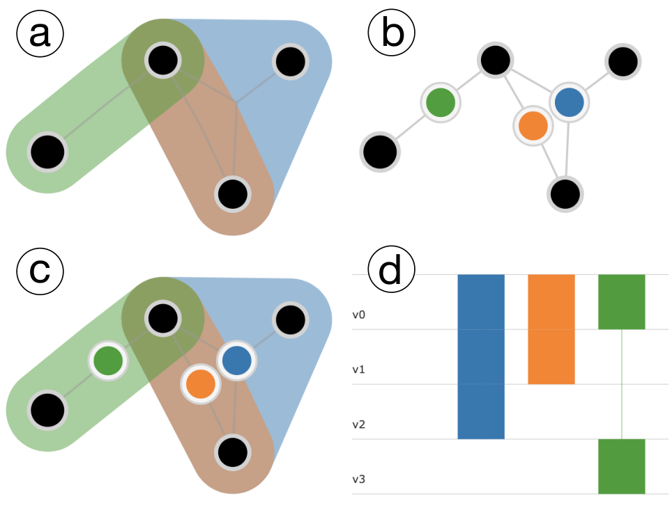
In all of these cases, exploration of the data can help discover interesting patterns, subsets, and entities. Graphs (or networks) are a central way to model data that come in the form of pairwise (or binary) relationships. However, graphs cannot natively represent multiway relationships without moving to bipartite structures or employing reification strategies. Instead, hypergraphs provide a way to capture these multiway interactions. A hypergraph, , consists of a set of vertices, , together with a collection of hyperedges, , each of which is a subset of vertices . For instance, Fig. 2a gives a hypergraph with 4 vertices and 3 hyperedges.
Visualization can be a useful tool to explore data modeled as hypergraphs. There are various visual encodings for a hypergraph. A Venn diagram based visualization (Fig. 2a) places vertices on the plane and represents hyperedges as convex hulls of the vertices. A bipartite graph based visualization (Fig. 2b) considers the set of hyperedges and the set of vertices as the two disjoint sets of a bipartite graph. A hybrid visualization combines both Venn diagram with bipartite graph based visualizations (Fig. 2c). And a rainbow box based visualization treats hyperedges (columns) as boxes (Fig. 2d).

Visualizing large graphs remains challenging as naive visualization often produces “hairballs” of little information content due to visual clutter. Such a problem is further compounded when dealing with hypergraphs, even ones with a moderate number of vertices and a small number of hyperedges. As the number of vertices grows and hyperedges become more interconnected, it becomes increasingly difficult to turn a naive visualization into insights. Fig. 3a illustrates a naive hypergraph visualization where vertices represent genes and hyperedges consist of pathways from the Hallmarks collection within the Molecular Signatures Database (MSigDB) [4, 5]. While vertices on the periphery are shown to belong to a single hyperedge, edge memberships of those vertices closer to the center are more difficult to interpret.


To reduce visual clutter, we might want to apply vertex collapse and hyperedge collapse to reduce the size of the hypergraph. As illustrated in Fig. 4, vertex collapse combines vertices that belong to exactly the same set of hyperedges into a single “super-vertex” (visualized by concentric ring glyph), while hyperedge collapse merges hyperedges that share exactly the same set of vertices into a “super-edge” (visualized by a pie-chart glyph). See Fig. 3b for the simplified biological pathway hypergraph after vertex collapse.
In this paper, we relax the notions of vertex collapse and hyperedge collapse by allowing vertices to be combined if they belong to almost the same set of hyperedges, and hyperedges to be merged if they share almost the same set of vertices. The former is referred to as the vertex simplification (or approximate vertex collapse), and the latter is referred to as the hyperedge simplification (or approximate hyperedge collapse). Using tools from topological data analysis, in particular, barcodes that capture the topology of hypergraphs, we perform topological simplification of hypergraphs. Our approach is general as it generalizes vertex and hyperedge collapses to their approximate versions. As we simplify a hypergraph in a way that removes topological noise as determined by its barcode, our approach is also mathematically justified by the stability of barcodes [6].
Our pipeline is illustrated in Fig. 1. To enable hyperedge simplification (Fig. 1 top), we first convert a hypergraph into a graph representation called the (weighted) line graph. A line graph captures the similarities among hyperedges. We then perform a topological simplification of the line graph. The simplified line graph induces a hyperedge simplification of the input hypergraph. On the other hand, to enable vertex simplification (Fig. 1 bottom), we first consider a (weighted) clique expansion of an input hypergraph. We then perform a topological simplification of the clique expansion. A clique expansion captures the similarities among vertices; it is known to be the line graph of the dual of a hypergraph. The simplified clique expansion in turn induces the vertex simplification of the input hypergraph. Using barcode-guided topological simplification, we formalize both vertex and hyperedge simplification in a unifying way.
We demonstrate the utility of our approach with real world examples. We provide an open source, interactive tool that includes modular and easily extendable implementation of our proposed algorithms. The tool allows users to explore the simplification framework by inputting their own datasets and applying vertex and hyperedge simplifications to gain insights from the data. The tool is open source via GitHub: https://github.com/tdavislab/Hypergraph-Vis.
II Related Work
We focus on visualization techniques relevant to hypergraphs. For graph visualization, see surveys on graph visualization for information visualization [7], graph representations for scientific visualization [8], visual analysis of large graphs [9], dynamic graphs [10], and graph drawing [11].
Mäkinen [12] introduced two widely used approaches for drawing hypergraphs. In an edge-based approach, hyperedges are drawn as smooth curves connecting their vertices. In a subset-based approach, they are drawn as closed curves enclosing their vertices. For the edge-based approach, by mapping a hypergraph to a graph, hypergraph visualization could be considered as an extension of graph visualization. Arafat et al. [13] proposed four different ways of encoding a hypergraph as a graph, via complete-, star-, cycle-, and wheel-associated-graphs. Paquette et al. [14] considered a hypergraph as a bipartite graph, where hyperedges and vertices form two disjoint and independent sets. For the subset-based approach, hypergraph visualization is closely related to set visualization (see [15] for a survey), which goes back to Euler diagrams [16] and its more restrictive form, the Venn diagrams. Kritz and Perlin [17] proposed the QUAD scheme that resembled a matrix encoding of set relations: each hyperedge is a column represented by a rectangle and each vertex is a point along a particular row. Simonetto et al. [18, 19] introduced an automatic generation of Euler-like diagrams (EulerView) for any collection of sets and their intersections. Many recent works focused on representing sets in more efficient ways, including LineSets [20], BubbleSets [21], MapSets [22], UpSet [23], and LinearDiagrams [24] etc. The rainbow box based visualization implemented in our tool is inspired by the work of Lamy [25], which visualized undirected graphs and symmetric square matrices by transforming them into overlapping sets, and visualized them with rainbow boxes. The HyperNetX Python package [26] includes hypergraph visualization using an Euler diagram approach. It also includes the ability to perform exact edge and vertex collapses (as opposed to approximate collapses which this current paper explores). Collapsed vertices and hyperedges are visualized in HyperNetX as larger “supervertices” and thicker “superedges”.
In terms of layouts, Valdivia et al. [27] introduced Parallel Aggregated Ordered Hypergraph (PAOH) as a hybrid of edge-based and subset-based (matrix) approach, which represents vertices as parallel horizontal bars and hyperedges as vertical lines, using dots to depict the connections to one or more vertices. Kerren and Jusufi [28] introduced a radial layout, where vertices are evenly distributed on a circle, and the hyperedges are represented as arcs that enclose the circle. Hypergraphs can be represented geometrically [29, 30], starting with Zykov [31]. Gropp [32] positioned the vertices in the plane such that those that form hyperedges are collinear in the plane. Evans et al. [33] used polygons to represent hyperedges in 3D to gain additional flexibility.
Evaluating hypergraph visualizations can be considered from a quantitative and a qualitative perspective. Many evaluation criteria for graph visualization are applicable for hypergraphs (e.g. [34, 35]), including aesthetic criteria such as readability [34] and faithfulness [35]. Mäkinen [12] gave a set of desirable aesthetic properties for subset-based hypergraph visualization. Arafat et al. [13] perfected these properties by introducing quantitative metrics such as concavity, planarity, and coverage metrics. In our work, we evaluate the quality of hypergraph visualizations after simplification using four different aesthetic criteria. The first criterion evaluates the Venn diagram based visualization, which is to minimize the approximate number of contour intersections. The remaining three criteria evaluate the bipartite graph based visualization, which aim to minimize the number of edge crossings [36], to minimize the normalized edge length variation [37], and to maximize the minimum angle between edges out from a node [36], respectively.
For graph simplification, a number of works focused on algorithmic developments [38, 39, 40] and visualization [41, 42, 43, 44, 45]. In particular, Suh et al. [46] proposed a topology-based graph simplification tool, which enables contraction of edges whose weight is below a user-specified threshold. There are only a few research works on hypergraph simplification. Lemonnier et al. [47] proposed a hypergraph simplification approach using notions from quantum physics. To the best of our knowledge, we are the first to use topological profiles to guide the hypergraph simplification process for visual exploration.
Finally, many research efforts have focused on visualizing large graphs with advanced hardwares such as GPUs, e.g., Graphistry (https://github.com/graphistry/), see [9] for surveys. Few works focus on large hypergraph visualization. We consider these scalable visualization approaches to be tangential to hypergraph simplification.
In this paper, we focus on increasing the readability while preserving as much as possible information faithfulness of hypergraph data via simplification. We apply vertex simplification and edge simplification to reduce the size of the hypergraph while preserving its information for insight discovery. It is important to emphasize that our simplification applies to any hypergraph visualization technique. We primarily use subset based approaches for hypergraph visualization, including Venn diagram, bipartite graph, and rainbow box based approaches (Fig. 2). While other visual encodings are possible for hypergraphs, we choose these approaches since the first two approaches capture spatial relations among the hyperedges, while the third approach highlights overlaps among the hyperedges.
III Technical Background
We review the definitions of hypergraphs and several graph representations highly relevant to hypergraphs, namely, dual hypergraphs, line graphs, and clique expansions. To explore graphs, one might employ network science measures such as centrality, clustering coefficient, and connected components to discover entities of interest. In this paper, we work with analogous hypernetwork science [48] concepts for hypergraphs, namely, -walks and -connected components.
III-A Hypergraphs, Line Graphs, and Clique Expansions
Definition III.1.
A hypergraph consists of a set of vertices, , and a family of hyperedges, ; where for .

Shown in Fig. 5a, is an example hypergraph with 5 black vertices and 3 colored hyperedges. It is specified by and . In most scenarios of this paper, a hypergraph is shown with the hybrid visualization, by superimposing Venn diagram and bipartite graph based visual encodings; black nodes are vertices, colored nodes and colored convex hulls represent hyperedges. For instance, in Fig. 5a, the blue hyperedge containing three black vertices (, , and ) is represented by a blue node as well as a blue convex hull.
As part of the pipeline for hypergraph simplification, we convert the hypergraph into a graph. There are two candidate graph representations of a hypergraph: the line graph [49] and the clique expansion [50]. The line graph of is a graph whose vertex set corresponds to the set of hyperedges of ; two vertices are adjacent in if their corresponding hyperedges have a nonempty intersection in . The clique expansion of constructs a graph from a hypergraph by replacing each hyperedge with a clique among its vertices. We formalize these concepts in the following two definitions.
Definition III.2.
The line graph of a hypergraph consists of a vertex set , and an edge set .
Definition III.3.
The clique expansion of a hypergraph consists of vertex set (the same vertex set as ), and there is an edge in if there exists some hyperedge such that .
The line graph and clique expansion are related through the concept of duality.
Definition III.4.
The dual hypergraph of has vertex set and hyperedge set , where .
As shown in Fig. 5c, swaps the roles of vertices and hyperedges. For instance, hyperedge in becomes vertex in , and vertex in becomes hyperedge in . It is not difficult to show that the clique expansion is the line graph of the dual, .
For our hypergraph simplification we work primarily with a weighted line graph or clique complex, using intersection sizes or Jaccard indices as weights. In the intersection weight of edge is while the Jaccard weight is . By duality, in the intersection weight of edge is and the Jaccard weight is .
The Jaccard weighted line graph, , of is shown in Fig. 5b. The hyperedges and in turn into vertices and in with weight on equal to .
The Jaccard weighted clique expansion is shown in Fig. 5d. For example, vertices and in belong to sets of edges and respectively. The edge in has a weight equal to .
In a nutshell, the Jaccard weighted line graph of a hypergraph captures the similarities between hyperedges; the higher the weights, the more similar they are. On the other hand, the Jaccard weighted clique expansion – the line graph of the dual hypergraph – captures similarities between vertices.
III-B -Walks and -Connected Components
For a graph , a walk of length is a sequence of vertices connected by edges. It can also be described as a sequence of successively incident edges. We include a similar notion of walk on a hypergraph, introduced by [48], using a hyperedge perspective.
Definition III.5.
An -walk of length between hyperedges and in a hypergraph is a sequence of hyperedges, , where for each , and .
Definition III.6.
For a hypergraph , a subset of hyperedges is -connected if there exists an -walk between all pairs of hyperedges in . is an -connected component if it is maximal, that is, there is no -connected set such that .

Definition III.7.
An -line graph of (for ), denoted as , is a filtered line graph where edge is present only if . Similarly, an -clique expansion of , denoted as , is a filtered clique expansion where edge is present only if and share at least hyperedges in .
The notion of -line graphs and -clique expansions allow us to filter a hypergraph by its connectivity, as illustrated in Fig. 6. For example, there is a -walk (dotted black arrow) between the red hyperdege to the green hyperedge via the blue hyperedge, as shown in Fig. 6d.
For the remainder of this paper, we work primarily with the Jaccard weighted -line graph of , denoted as , and the Jaccard weighted -clique expansion of , denoted as . Unless otherwise stated, . In one of our examples we will provide a comparison between edge weights based on the Jaccard indices and the intersection size.
III-C Topological Simplifications of Graphs
In this section, we first introduce the topological profile of a weighted graph, formally known as its barcode [51, 52], which is grounded in persistent homology [53]. We then use the barcode to guide the topological simplification of the graph. Later, in Sect. IV, we show how simplification of graphs and are used to perform our hypergraph simplification.
To obtain the barcode of a weighted graph , we apply persistent homology to a metric space representation of the graph [54]. See [55] for an introduction and [51] for an algebraic treatment of persistent homology. Persistent homology can be used to capture topological features (e.g., connected components, loops, and higher dimensional voids) in any dimension, . In this paper we will focus on , allowing us to simplify the definition of a barcode since this restricted version can be computed using the notion of a minimum spanning tree (MST) of a graph. In other words, a merger of two components corresponds to an edge of the MST. Recall an MST is a spanning tree with minimum possible total edge weight. As an MST can also be used to derive the single linkage clustering (SLC) dendrogram [56], the barcode-guided simplification process is also equivalent to applying the SLC with a threshold.

A weighted graph, , consists of vertices, , edges, , and a weight function . Constructing an MST will tend to keep edges with smaller weight and remove those with higher weight. Typically this is done because the weights represent distances, where a small weight means two vertices are close, or similar, and a large weight means two vertices are far, or dissimilar. In the case that weights are similarities, not distances, two vertices with high weight are more similar than two with low weight. To simplify a similarity-weighted graph, we wish to merge vertices in into super-vertices based on a decreasing order of their similarities. Therefore, before computing the barcode of , we first invert each edge weight to be and then compute the corresponding MST.
The barcode is a visual representation of the MST that consists of a collection of sorted horizontal line segments (bars) in a plane, where each line segment (excluding the longest one) corresponds to an edge in the MST with length proportional to its weights. As illustrated in Fig. 7a, four of the thickest edges (shown with edge weights) form the MST; each of these edges gives rise to a bar in the barcode in Fig. 7d. For instance, the edge connecting the most similar vertices – the red and the purple vertices (pointed by arrows) – in Fig. 7a with a weight of gives rise to the shortest bar of length in Fig. 7d.
Suh et al. [46] used the barcode to control the contraction and repulsion of edges in the force-directed layout of a graph. Instead, in this paper, we use the barcode to guide the merging of vertices into super-vertices as part of the simplification pipeline. As illustrated in Fig. 7e, if we choose a threshold that passes the first bar, we combine the purple and red vertices together into a super-vertex in (b). Similarly, choosing a threshold that passes the second bar in Fig. 7f results in the combination of purple, red, and pink vertices into a super-vertex in (c).
Stability. We consider a barcode-guided simplification of a graph to be mathematically justified in the following sense. We call a graph an -simplification of another graph , if is obtained from via vertex contractions (that is, merging subsets of vertices in thus contracting the induced edges), and the barcode is the same as the barcode except all bars with lengths at most have been removed. Based on the stability of barcodes [6], by performing a simplification up to a threshold of , the distance between the barcodes of and is upper bounded by .
Formally, let be a matching between the intervals (bars) and of and respectively, define the bottleneck distance between and to be
where distance between two bars and is defined as . In our setting, the distance between two bars that start at zero, and , is the absolute difference of their end points, . Then we have the stability of barcodes,
By construction, the MST of is generated from the MST of by contracting edges with lengths at most , therefore merging vertices connected by these edges that are at most apart. Therefore, and only differ by the bars that are removed via the simplification, which have lengths at most .
IV Methods
We now describe multi-scale topological simplifications of hypergraphs. We use the term vertex (resp. hyperedge) simplification to mean a sequence of operations that reduce the size of a hypergraph by merging vertices (resp. hyperedges) in decreasing levels of similarity. Our framework is as follows:
- 1.
Map a hypergraph to a graph representation ;
- 2.
Generate the barcode of and use to guide its simplification;
- 3.
A simplified induces a simplification of .
At the core of our approach is the idea that a simplified clique expansion induces a vertex simplification of the hypergraph, while a simplified line graph induces a hyperedge simplification. Using barcodes of these weighted graph representations, we allow vertices to be combined if they belong to almost the same set of edges, and edges to be merged if they share almost the same set of vertices, both in a mathematically justifiable way.

There are two parameters that guide the simplification process. First, the parameter gives rise to a filtered version of the line graph or the clique expansion. Fig. 6 illustrates a multi-scale filtering of hyperedges using parameter, for and respectively.

Second, the parameter used in the -simplification of a hypergraph by merging vertices (or hyperedges) whose distances are upper bounded by (corresponding, whose similarities are lower bounded by ). Fig. 8 illustrates multi-scale hyperedge simplifications. At , the brown and purple hyperedges merge into one (pointed by a black arrow); and at , three hyperedges in red, green, and blue merge into one at the same time (pointed by the hollow arrow). Fig. 9 illustrates multi-scale vertex simplifications. At , the grey and pink vertices in the clique expansion (that correspond to the two vertices in the orange hyperedge) merge into one super-vertex (pointed by a black arrow); and at , two vertices in purple and teal in the clique expansion merge into a super-vertex (pointed by a hollow arrow).
V Interactive Visualization System
We provide an open source, interactive visualization system that supports both vertex and hyperedge simplification of an input hypergraph. Its user interface is shown in Fig. 10, see the supplementary video for a demo. We describe the interface based on hyperedge simplification; the interface for vertex simplification is similar with minor modifications.
In the middle, the graph visualization panel visualizes the original hypergraph (a), the weighted line graph representation (b), the simplified line graph (d), and the induced simplified hypergraph (c), in Fig. 10 respectively. The vertices and (hyper)edges across (a-d) are connected via linked views based upon their correspondences. When we switch from hyperedge simplification to vertex simplification, weighted line graph representations (b, d) become weighted clique expansions accordingly.

On the left, the barcode panel (e) controls the level of simplification (parameter ) for the line graph where vertices connected by edges with weight below the selected threshold in (b) are combined into super-vertices in (d). Correspondingly, hyperedges in (c) are merged into one hyperedge. Panel (e) also shows the hierarchical merging of hyperedges (or vertices) via a dendrogram. It further performs refinement of a simplified hypergraph via the bar expansion: clicking on a bar that has already been simplified will undo the simplification step. This means, if hyperedges and have been merged into a single hyperedge under the current simplification level, clicking the bar that corresponds to this operation will separate back into and . To choose the right simplification level, the lower part (f) of the panel displays the labels of hyperedges (or vertices) when hovering on a simplified hyperedge (or vertex). Alternatively, it can also display the persistence graph (not shown here) that shows the number of features (connected components) as a function of the persistence level . An appropriate value of is typipcally obtained at the plateau of the persistence graph (see [57] for details).
On the right, the visual encoding control panel (g) provides various visual encodings for the hypergraph, see Fig. 2 for an example. The panel also provides options to display vertex and hyperedge labels. The parameter control panel (h) deals with parameter configuration. A large input hypergraph can be pre-processed to allow vertex collapse and hyperedge collapse. It is important to point out that collapsing the hypergraph here affects the weights in the line graph or clique expansion, which in turn affects the barcode. If two edges intersect in vertices, and those vertices are collapsed into super-vertices, then the weight between those hyperedges will be , not . Choosing edge simplification employs the line graph representation, while vertex simplification uses the clique expansion. The parameter controls the edges present in the -line graph or -clique expansion. Singletons in the -line graph or -clique expansion are either greyed out (used in barcode computation but visualized as light gray) or filtered (removed from the hypergraph visualization and not used in barcode computation). In computing the barcodes, either Jaccard index or overlap size can be used. All of the parameters set in panel (h) contribute to barcode computation. Any change made to the parameters requires a re-computation of the barcode by clicking compute barcode.
Implementation. We implemented our framework as an interactive web application with a Python back-end using a Flask-based server. We use the standard HTML/CSS/Javascript stack in tandem with D3.js and JQuery JavaScript libraries for designing the user interface and visualization panels. The front-end handles data upload, graph and hypergraph visualization, and it sends information about parameter modifications to the back-end. The Python back-end handles data parsing, creating the hypergraph data structures using the HyperNetX [26] library (including its edge and vertex collapse functions), constructing bipartite graphs, computing the persistence barcodes, and parameter updates. The front-end and back-end communicate using AJAX requests and the data is transferred using JSON format.
VI Results
We provide five example use cases to show how our barcode-guided hypergraph simplification provides an interpretation of the underlying data and helps with insight discovery.
VI-A Southern Women
Our first example considers a small social network. In the 1930s, a group of ethnographers collected data on a group of 18 women in Natchez, Mississippi [58]. They recorded attendance at 14 informal social events over the course of a nine month period; see Fig. 11. This dataset has been studied by many other researchers in sociology, information theory, and mathematics, see [59] for a meta-analysis of previous studies.


The hypergraph of this dataset is shown in Fig. 12a. Through interviews with these women, Davis et al. [58] identified two largely distinct groups and determined core, primary, and secondary members of each group based on how they were involved with the events, as summarized in Fig. 12b. Such groupings are considered as the ground truth in our exploration. The original layout of the hypergraph in Fig. 12a gives the illusion of a left-right split of the groups, while the ground truth indicates a top-bottom split, where Pearl (red circle) belongs to Group 1, Dorothy (blue circle) belongs to Group 2, and Ruth (green circle) is identified as secondary in both groups.
Using this Southern Women dataset, we will demonstrate how varying parameter choices using our system affects the simplification results, and in some scenarios, highlights the group relations within the ground truth. We will observe which parameter choices agree with the reported ground truth and which do not. In all cases we will perform vertex simplification as the goal is to see how the women are grouped based on the events they attend.
Simplification using Jaccard weights. We first consider vertex simplification of the Jaccard weighted clique expansion derived from the original hypergraph with .
As we increase our simplification parameter , guided by a priori knowledge of the group structure, we observe that at (Fig. 13a & d), super-vertices are formed mostly according to the core groups from the ground truth, with Group 1 core members on the right (the hyperedge pointed by a filled arrow, Laura, Brenda,Evelyn, Theresa), most of the Group 2 core and primary members on the left (the hyperedge pointed by a double filled arrow, Myrna, Nora, Sylvia, Katherine), and Ruth in the middle.

As illustrated in Fig. 13a, all super-vertices consist of members of the same group, with the exception of Pearl and Dorothy (Group 1 and Group 2 secondary respectively, hollow arrow). Flora and Olivia form a hyper-vertex, since they attended exactly the same set of two events (cf. Fig. 11, double hollow arrow). All of the core members of Group 1 (Laura, Brenda, Evelyn, Theresa) are merged together into a super-vertex (filled arrow). Almost all core and primary members of Group 2 (Myrna, Nora, Sylvia, Katherine, minus Helen) form a second super-vertex (filled double arrow).
We further hypothesize that after simplifying down to two super-vertices, each super-vertex would correspond to a group in the ground truth. However, this is not the case as shown in Fig. 13b. In the simplified hypergraph, one super-vertex contains only Flora and Olivia; while the other super-vertex contains everyone else.
Finally, we increase the value to , filter out singletons, and simplify to two remaining super-vertices. The result is shown in Fig. 13c. This filtering process leaves out Dorothy, Olivia, Flora, and Pearl (all of whom are secondary members), but otherwise splits the women into the correct two groups. The left super-vertex (filled arrow) consists of Group 2 core and primary members and Verne (Group 2 secondary). The right super-vertex (filled double arrow) similarly consists of Group 1 core and primary members and Ruth (Group 1 & 2 secondary).
In summary, simplification using the Jaccard weights and is unable to identify the two groups in the ground truth without using the a priori knowledge. Using , we could identify two subgroups appropriately, however certain secondary members are filtered out unintentionally. Next we compare with simplification results using overlap weights.
Simplification using overlap weights. We first simplify the overlap weighted clique expansion by setting . As we increase , the simplification process clearly identifies the two subgroups in the ground truth, see Fig. 14a with the corresponding merging hierarchy in Fig. 11 (right). It identifies the same split as in Fig. 13c without filtering Pearl, Dorothy, Flora, and Olivia. In particular, the right hyper-vertex (filled arrow) contains all core and primary members of Group 2 plus its secondary member Verne; and the left hyper-vertex (filled double arrows) contains all core and primary members of Group 1 plus Ruth. Flora and Olivia are combined as usual.
As we increase further, we simplify down to three super-vertices, see Fig. 14b. There is no threshold with two super-vertices as the final simplification merges all three into one super-vertex. As in the case of Jaccard weights, this naive simplification does not achieve the desired split into the correct groups. Flora and Olivia are again grouped together, Dorothy is on her own, and everyone else is grouped together.
Finally, we increase the value again to . It shows the same split as Fig. 14a, while again filtering Pearl, Dorothy, Flora, and Olivia.

Final remarks. In this small example with ground truth, we are able to see how Jaccard and overlap weights perform slightly differently. The fact that it is easier to identify the two groups using overlap weights may be an artifact of how the two groups were identified in the first place by Davis et al. through interviews and sociological observations. Hence we cannot expect such an observation to be generalized to other datasets. It is clear from this example that Jaccard and overlap weights perform differently and may help provide different insights into the same dataset. In crafting the examples in the following subsections we explored each dataset using a variety of parameter and weight choices and will show the choice that provided the most insight. It happens that Jaccard weights are used in all of the remaining examples.
VI-B Les Misérables
Our second example considers Victor Hugo’s novel Les Misérables, as broken down in the file jean.dat from the Stanford Graph Base [60]. This dataset lists the set of characters found within each volume, book, chapter, and scene of the story. To form our hypergraph, we consider each character to be a vertex and each (volume, book)-pair to be a hyperedge containing those characters that appear within. We use the following parameter settings for the simplification: collapse vertices and edges; vertex simplification; ; filter singletons; and Jaccard weighted edges. Fig. 15 shows the simplification results.

It is not possible to go through the entire plot of this very long novel here, but the story of Les Misérables revolves around the characters of Jean Valjean, Javert, Cosette, and Fantine (labeled in Fig. 15b). Other characters of interest include Cosette’s love interest Marius (also labeled in Fig. 15b), a revolutionary student club, and some others that get mixed up in an uprising. Our vertex simplification groups many characters together in interesting ways that reflect the narrative of this story.
In the simplified hypergraph Fig. 15c, a vertex (character) of interest is the fact that Fantine, one of the characters many consider a main character in the novel, does not group with her daughter Cosette or any other main character. In hindsight, this makes sense, since Fantine appears only in the first volume (of five) and acts as a bridge from the first volume to the rest of the story, losing her daughter Cosette early on. Fantine remains an unsimplified vertex (not grouped with any other characters) since she interacts with many groups that do not interact with each other. This makes her Jaccard similarity to all of these groups low.
Fig. 15(d-f) show and describe correspondences between three of the super-vertices in the simplification (, and , pointed by arrows in Fig. 15c) with the vertices of the original hypergraph (Fig. 15a). The super-vertex from Fig. 15c contains many peripheral characters in the first volume in Fig. 15d, those that interact with Jean Valjean and Fantine. The super-vertex contains all of the “Friends of the ABC” revolutionary student group (circled in red) plus two street kids (circled in blue) that get mixed up in the uprising and two additional prominent uprising characters (circled in purple), see Fig. 15e. The super-vertex from Fig. 15c contains Jean Valjean, Cosette, Javert, Marius, and all of Marius’ family (circled in orange), see Fig. 15f.
Finally, we can use the bar expansion capability to explore the two bars that are merged just before our chosen threshold (). Fig. 16a shows that expanding one bar splits the super-vertices containing Marius and his family from the one containing Jean Valjean, Cosette, and Javert. In Fig. 16b, we see that expanding the second bar further splits Valjean and Cosette from Javert. Both of these operations make sense in the context of the story. While all of these characters interact frequently, Valjean and Cosette are certainly the closest and most central pair in the story. Moreover, Javert is always chasing Valjean so they do not interact as much, instead they each interact with the same intermediate characters.

While this barcode-guided simplification does not capture the complete narrative flow of the story from beginning to end, it does group characters in ways that align with the story. It also shows how various smaller groups interact with each other as smaller groups merge to form larger groups, and how some characters act as bridges between others.
VI-C Hallmarks Biological Pathways
Our third example explores the Hallmarks biological pathways hypergraph [4] as shown in Fig. 3. The full Hallmarks dataset contains 50 pathways (hyperedges) and 4,386 genes (vertices). We first use HyperNetX to break this large hypergraph into 2-connected components in order to focus on a smaller subset for visual exploration. We chose a component that contains 10 hyperedges. Throughout this example, biological information about pathways is obtained online from MSigDB [4, 5].


For this example, we use the following parameter settings: do not collapse vertices or edges; edge simplification; ; grey out singletons; and Jaccard weights. Rather than choosing one threshold for simplification as in the previous example, we will show insights gathered by walking through the various thresholds to see the order in which the hyperedges (pathways) merge. The original Hallmark hypergraph and the vertex collapsed hypergraph is shown in Fig. 3. In Fig. 17, we show the vertex collapsed hypergraph by treating collapsed vertices as single vertices along with the initial barcode for this simplification process.
Fig. 18(a-d) shows the first four steps of the simplification process from left to right. The 1st two hyperedges (pathways) to merge are INTERFERON_ALPHA_RESPONSE and INTERFERON_GAMMA_RESPONSE (Fig. 18a). Both are pathways that contain genes up-regulated in response to interferon (resp. alpha or gamma) proteins. The 2nd pair (Fig. 18b) to merge are HYPOXIA (genes up-regulated in response to low oxygen) and GLYCOLYSIS (genes involved in breaking down glucose). Unlike the 1st pair of edges, the processes of hypoxia and glycolysis are not very related, but they are merged early in the process so they must have many genes in common. An observation that may be useful for biology researchers. The 3rd bar guides the merging of INFLAMMATORY_RESPONSE with TNFA_SIGNALING_VIA_NFKB (genes regulated by NF-kB in response to TNF), see Fig. 18c. The NF-kB protein complex and TNF protein are both known to play a role in regulation of immune response so a merge with an inflammatory response is reasonable. The 4th step merges the INTERFERON pair in (a) with the INFLAMMATORY and TNFA pair in (c) and the ALLOGRAFT_REJECTION pathway, which is involved with transplant rejection. This new super-hyperedge seems to encompass all of the inflammatory response edges present within or original set of 10.
At this point, we have five (super-)hyperedges in our simplified hypergraph: inflammation/immune pathways; hypoxia and glycolysis; APOPTOSIS (programmed cell death); MTORC1_SIGNALING (related to mTORC1 complex involved in protein synthesis); and P53_PATHWAY (related to cancer suppression). In the next four steps of the simplification (1) APOPTOSIS merges with the inflammation/immune hyperedge, (2) MTORC1 merges with hypoxia and glycolysis, (3) those two just created super-edges merge together, and (4), P53 merges in last.
This simplification process provides a merging hierarchy amongst these 10 pathways, see Fig. 19. While MSigDB provides pairwise overlap sizes for all of these pathways, the most important insight using our framework is that our simplification process goes beyond pairwise associations and hierarchically merges pathways to discover groups of related pathways.

VI-D ActiveDNS
Our fourth example is from computer networking, specifically the Domain Name System (DNS). DNS focuses on how computers translate from the human interpretable domains (e.g., www.google.com) to computer-readable IP addresses (e.g., 192.168.1.1). It might seem like these should be one to one, that is, each domain has an IP address, and each IP maps to a domain, but this is not always the case. Domain aliasing means that sometimes multiple domains map to the same IP (misspellings like www.gogle.com still get you to the right place) and website hosting services mean that multiple domains can be served up from the same IP address. The way that IPs are allocated to domains can show interesting patterns. Using a hypergraph representation of the data, where vertices are IP addresses and edges are domains, we ask the question of whether or not domains that share many common IP addresses have any common properties.
The dataset for this exploration comes from ActiveDNS [61]. This project out of Georgia Tech does daily active DNS lookups for millions of IP addresses and records the query results in a database. We work with one day of DNS records, from April 26, 2018, as our test case. This data was also explored as a hypergraph in [1]. The entire hypergraph from this day has millions of vertices and edges so we first used the Chapel Hypergraph Library (CHGL) [62, 63] to break the hypergraph into two connected components and then chose one of these components which has 30 hyperedges (domain names) to explore visually using our framework. The original hypergraph is shown in Fig. 20a and the collapsed in Fig. 20b.

For the simplification, we use the following parameters: collapse vertices and edges; edge simplification; ; grey out singletons; and Jaccard weight. We chose to get more to the core of the interactions within this component. The barcode (with the chosen threshold), and the resulting simplified hypergraph, are shown in Fig. 20c and Fig. 20d respectively.
As shown in Fig. 20d, the simplified hypergraph shows a clear separation into two main super-hyperedges, green (filled arrow) and orange (filled double arrow), with one additional yellow hyperedge (hollow arrow) that is fully contained within the green. There are also 4 greyed out hyperedges which are not 3-connected to the rest of the component. The separation is also evident in the original and collapsed hypergraphs but the groupings become more obvious in the simplified version. After making this observation, we use the WHOIS lookup from Hurricane Electric BGP Toolkit [64] to answer the question of what the domains that are grouped have in common. WHOIS gives publicly available information about the organization that registered the domain, their contact information, and a variety of other metadata.
Fig. 20e highlights the 14 edges in the original hypergraph that are collapsed to form the orange edge in the simplified version. The domain names (hyperedges) that are collapsed include worldsleadingcruiselines.com, worldsleadingcruiselines.net, wlcl.com, and worldleadingcruiseline.com. In fact, all 14 are some play on “World’s Leading Cruise Lines” and all domains are registered to Carnival Corporation which is, in fact, one of the world’s largest cruise lines. Interestingly, one of the grayed out hyperedges has the domain comebacktothesea.com. “Come Back to the Sea” is an older advertising campaign for Carnival and perhaps that is why it does not have as much overlap with the other domains with the more current slogan.
The 11 edges highlighted in Fig. 20f, which are collapsed to form the green edge in the simplified version, have less in common on the surface. These domains include bbgdirect.com, azattykplus.kg, and globalnewsdashboard.com. Within these 11 domains, 7 of them have “Radio Free Europe” listed as the registered organization in the publicly available WHOIS information, two have no registered organization, and two have completely different organizations. Finally, the yellow edge that is contained within the green in Fig. 20c has domain radiosvobodakrim.mobi and is also registered to “Radio Free Europe.” We make no claims of associations between these domains, especially those registered to other organizations. We only observe that our hypergraph simplification method grouped domains together that, for the most part, were registered by the same organization.
VI-E Coauthor Networks
Our final example concerns a coauthorship network in academic publications. We use the topic-coauthor dataset from ArnetMiner [65] and focus specifically on the information-retrieval field-of-study for authors. Each hyperedge represents an author and vertices in the corresponding hyperedge are researchers who have coauthored at least one paper with the author. There are 491 hyperedges and 1907 vertices in this hypergraph. For this exploration, we use the following parameter setting: do not collapse edges or vertices, edge simplification, , grey out singletons, Jaccard weights, and . Fig. 21a shows the unsimplified hypergraph, and though there seems to be a central clustering affinity, it is very hard to parse the information in a hypergraph of this size.

Contrast this with the simplified hypergraph (at , ) in Fig. 21b, where the centrality of authorship is clearly evident. The central node (filled arrow) is the result of merging hyperedges under our framework. The edges in this node correspond to prolific researchers in information retrieval with a high number of citations. In particular, as illustrated by the rainbow box based visualization of the simplified hypergraph in Fig. 21c, the central node consists of a hyperedge corresponding to David A. Grossman and Ophir Frieder who are the authors of the book “Information Retrieval: Algorithms and Heuristics”, an important introductory textbook of the field.
| Datasets | ||||||||||||
|---|---|---|---|---|---|---|---|---|---|---|---|---|
| B | A | B/A | B | A | B/A | B | A | B/A | B | A | B/A | |
| Southern Women | 164 | 139 | 1.18 | 0.94 | 0.95 | 0.99 | 0.05 | 0.08 | 0.625 | 0.32 | 0.46 | 0.70 |
| Les Misérables | 1246 | 962 | 1.30 | 0.98 | 0.94 | 1.04 | 0.04 | 0.06 | 0.67 | 0.56 | 0.54 | 1.04 |
| Hallmarks Biological Pathways | 554 | 120 | 4.62 | 0.99 | 0.92 | 1.08 | 0.01 | 0.02 | 0.5 | 0.88 | 0.48 | 1.83 |
| ActiveDNS | 656 | 51 | 12.86 | 0.96 | 0.93 | 1.03 | 0.04 | 0.13 | 0.31 | 0.45 | 0.58 | 0.78 |
| Coauthor Networks | 26162 | 278 | 94.11 | 0.98 | 0.99 | 0.99 | 0.02 | 0.05 | 0.4 | 0.67 | 0.86 | 0.78 |
VII Evaluation
It is important to note that the main contribution of this paper is the topology-based simplifications of hypergraphs, which can be used for any hypergraph visualization technique. In other words, hypergraph simplification is considered orthogonal to hypergraph visualization. On the other hand, to demonstrate the effectiveness of such simplifications, we evaluate the quality of hypergraph visualizations from Sect. VI using four different aesthetic criteria detailed below.
Contour intersections. Given a Venn diagram based visualization of a hypergraph , a contour intersection is a crossing of the boundaries of two convex hulls representing two hyperedges. To compute the number of contour intersections, we approximate the boundary of each convex hull using piecewise linear segments. The approximated contour intersections, denoted as , is defined as the number of intersections among these line segments.
Number of edge crossings. Given a bipartite graph based visualization of a hypergraph , we compute its number of edge crossings, denoted as , which is an aesthetic criterion first proposed by Purchase [36]. For the bipartite graph representation of with vertex set and edge set , is defined as
where is the number of edge crossings, and is the approximation of the upper bound of the number of edge crossings. is defined as
where is the degree of a vertex . Therefore, , and when there are no edge crossings in the bipartite graph.
Normalized edge length variation. We also evaluate the bipartite graph visualization of a hypergraph using the normalized edge length variation [37], denoted as . For a graph with a vertex set and an edge set , Hachul and Jünger [66] proposed a normalized standard deviation of the edge length ,
where is the length of an edge , and is the mean of the edge length. Kwon et al. [37] then proposed a normalized version of , which is to divide by its upper bound , and the normalized edge length variation is then defined as
By definition, . when all edge lengths are equal.
Minimum angle. Finally, we work with the the minimum angle between adjacent edges leaving a node [36], denoted as . Given a vertex , is defined based on the deviation of the minimum angle between the adjacent incident edges from the ideal minimum angle , where . The average absolute deviation of minimum angles is defined as
and the minimum angle metric is defined as
By definition, . when all the nodes have equal angles between all adjacent incident edges.
Evaluation results. We compute the above four criteria to evaluate the resulting hypergraph visualizations in Sect. VI that are either based on the Venn diagram or the bipartite graph. For each hypergraph, we compute a given criterion before and after simplification using the visualizations generated automatically by our tool without any modification. We also compute the ratio of the reported values before and after simplification for comparison. The last three criteria are computed using GLAM (https://github.com/VIDILabs/glam).
The evaluation results are shown in Table I. As shown in the table, our hypergraph simplification greatly improves the approximated number of contour intersections (), in particular, for large and complex hypergraphs (e.g., the Coauthor Networks). This is indicated by a large ratio that ranges between and in the table. Meanwhile, we obtain comparable numbers of edge crossings for the bipartite graph visualization before and after simplification. This is indicated by a ratio before and after simplification. On the other hand, a bipartite graph visualization of the simplified hypergraph shows slightly higher normalized edge length variation (). However, we consider this to be acceptable since all values are very close to (ranging from to across all datasets). Finally, we observe that we improve upon the minimum angle criterion for three out of five of the datasets with the simplification.
VIII Discussion
In this paper, we introduce a framework that supports topological simplification of hypergraphs via both vertex and edge simplifications. We exploit the duality between hypergraphs, line graphs, and clique expansions; and apply barcode-guided simplification of a hypergraph across multiple scales. We expect our framework to be applicable for general hypernetwork science (e.g. to be integrated with HyperNetX [26]). There are several interesting venues for future research.
We map a hypergraph to a metric space representation, where we use a shortest path metric in our current framework. There are other notions of metrics, in particular, resistance distance [67], commute time distance [68], and diffusion distance [69], which are applicable in our unifying framework (see Sect. IV). These metrics can be particularly interesting as they capture structural or physical properties of the underlying data.
As the barcode used to guide the simplification can be obtained by computing the minimum spanning tree, the simplification process is equivalent to applying a single-linkage clustering with a threshold. Some other clustering approaches, such as average-linkage clustering and complete-linkage clustering, or more complex methods using hypergraph Laplacians [70] or modularity [71], might also be used to guide hypergraph simplifications. A comparison among these clustering approaches will be interesting. Finally, it will be interesting to explore hypergraph simplification using higher dimensional barcode.
Acknowledgments
This project was partially supported by NSF IIS 1513616 and DOE DE-SC0021015.
References
- [1] C. A. Joslyn, S. Aksoy, D. Arendt, J. Firoz, L. Jenkins, B. Praggastis, E. A. Purvine, and M. Zalewski, “Hypergraph analytics of domain name system relationships,” in Procceedings of the 17th Workshop on Algorithms and Models for the Web Graph, Lecture Notes in Computer Science, 2020.
- [2] M. Ashburner, C. A. Ball, J. A. Blake, D. Botstein, H. Butler, J. M. Cherry, A. P. Davis, K. Dolinski, S. S. Dwight, J. T. Eppig, M. A. Harris, D. P. Hill, L. Issel-Tarver, A. Kasarskis, S. Lewis, J. C. Matese, J. E. Richardson, M. Ringwald, G. M. Rubin, and G. Sherlock, “Gene ontology: tool for the unification of biology,” Nature Genetics, vol. 25, no. 1, pp. 25–9, 2000.
- [3] The Gene Ontology Consortium, “The gene ontology resource: 20 years and still GOing strong,” Nucleic Acids Research, vol. 47, no. D1, pp. D330–D338, 2019.
- [4] A. Liberzon, C. Birger, H. Thorvaldsdóttir, M. Ghandi, J. P. Mesirov, and P. Tamayo, “The molecular signatures database hallmark gene set collection,” Cell systems, vol. 1, no. 6, pp. 417–425, 2015.
- [5] A. Subramanian, P. Tamayo, V. K. Mootha, S. Mukherjee, B. L. Ebert, M. A. Gillette, A. Paulovich, S. L. Pomeroy, T. R. Golub, E. S. Lander, and J. P. Mesirov, “Gene set enrichment analysis: A knowledge-based approach for interpreting genome-wide expression profiles,” Proceedings of the National Academy of Sciences, vol. 102, no. 43, pp. 15 545–15 550, 2005.
- [6] D. Cohen-Steiner, H. Edelsbrunner, and J. Harer, “Stability of persistence diagrams,” Discrete & Computational Geometry, vol. 37, pp. 103–120, 2007.
- [7] I. Herman, G. Melancon, and M. S. Marshall, “Graph visualization and navigation in information visualization: A survey,” IEEE Transactions of Visualization and Computer Graphics, vol. 6, no. 1, pp. 24–43, 2000.
- [8] C. Wang and J. Tao, “Graphs in scientific visualization: A survey,” Computer Graphic Forum, vol. 36, no. 1, pp. 263–287, 2017.
- [9] T. Von Landesberger, A. Kuijper, T. Schreck, J. Kohlhammer, J. J. van Wijk, J.-D. Fekete, and D. W. Fellner, “Visual analysis of large graphs: State-of-the-art and future research challenges,” Computer Graphics Forum, vol. 30, no. 6, pp. 1719–1749, 2011.
- [10] F. Beck, M. Burch, S. Diehl, and D. Weiskopf, “The state of the art in visualizing dynamic graphs,” EuroVis STARs, vol. 2, 2014.
- [11] P. Eades and R. Tamassia, “Algorithms for drawing graphs: An annotated bibliography,” Computational Geometry: Theory and Applications, vol. 4, no. 5, pp. 235–282, 1994.
- [12] E. Mäkinen, “How to draw a hypergraph,” International Journal of Computer Mathematics, vol. 34, no. 3-4, pp. 177–185, 1990.
- [13] N. A. Arafat and S. Bressan, “Hypergraph drawing by force-directed placement,” in International Conference on Database and Expert Systems Applications, 2017, pp. 387–394.
- [14] J. Paquette and T. Tokuyasu, “Hypergraph visualization and enrichment statistics: How the EGAN paradigm facilitates organic discovery from big data,” in Human Vision and Electronic Imaging XVI, vol. 7865, no. 78650E. International Society for Optics and Photonics, 2011.
- [15] B. Alsallakh, L. Micallef, W. Aigner, H. Hauser, S. Miksch, and P. Rodgers, “The state-of-the-art of set visualization,” Computer Graphics Forum, vol. 35, no. 1, pp. 234–260, 2016.
- [16] L. Euler, “Lettres á une princesse d’allemagne,” Letters 102-105, 1761.
- [17] M. Kritz and K. Perlin, “A new scheme for drawing hypergraphs,” International journal of computer mathematics, vol. 50, no. 3-4, pp. 131–134, 1994.
- [18] P. Simonetto, D. Auber, and D. Archambault, “Fully automatic visualisation of overlapping sets,” Computer Graphic Forum, vol. 28, no. 3, pp. 967–974, 2009.
- [19] P. Simonetto, “Visualisation of overlapping sets and clusters with Euler diagrams,” Ph.D. dissertation, University of Bordeaux, 2011.
- [20] B. Alper, N. Riche, G. Ramos, and M. Czerwinski, “Design study of linesets, a novel set visualization technique,” IEEE transactions on visualization and computer graphics, vol. 17, no. 12, pp. 2259–2267, 2011.
- [21] C. Collins, G. Penn, and S. Carpendale, “Bubble sets: Revealing set relations with isocontours over existing visualizations,” IEEE Transactions on Visualization and Computer Graphics, vol. 15, no. 6, pp. 1009–1016, 2009.
- [22] A. Efrat, Y. Hu, S. G. Kobourov, and S. Pupyrev, “MapSets: Visualizing embedded and clustered graphs,” Journal of Graph Algorithms and Applications, vol. 19, no. 2, pp. 571–593, 2015.
- [23] A. Lex, N. Gehlenborg, H. Strobelt, R. Vuillemot, and H. Pfister, “UpSet: visualization of intersecting sets,” IEEE Transactions on Visualization and Computer Graphics, vol. 20, no. 12, pp. 1983–1992, 2014.
- [24] P. Rodgers, G. Stapleton, and P. Chapman, “Visualizing sets with linear diagrams,” ACM Transactions on Computer-Human Interaction, vol. 22, no. 6, pp. 1–39, 2015.
- [25] J.-B. Lamy, “Visualizing undirected graphs and symmetric square matrices as overlapping sets,” Multimedia Tools and Applications, vol. 78, no. 23, pp. 33 091–33 112, 2019.
- [26] B. Praggastis, D. Arendt, E. Purvine, C. Joslyn, M. Raugas, S. Aksoy, and K. Monson, “HyperNetX,” https://github.com/pnnl/HyperNetX, 2018.
- [27] P. Valdivia, P. Buono, C. Plaisant, N. Dufournaud, and J.-D. Fekete, “Analyzing dynamic hypergraphs with Parallel Aggregated Ordered Hypergraph visualization,” IEEE Transactions on Visualization and Computer Graphics, vol. 27, no. 1, pp. 1–13, 2021.
- [28] A. Kerren and I. Jusufi, “A novel radial visualization approach for undirected hypergraphs,” in Proceedings of the 17th Eurographics Conference on Visualization, Short paper track, 2013.
- [29] U. Brandes, S. Cornelsen, B. Pampel, and A. Sallaberry, “Path-based supports for hypergraphs,” Journal of Discrete Algorithms, vol. 14, pp. 248–261, 2012.
- [30] K. Buchin, M. van Kreveld, H. Meijer, B. Speckmann, and K. Verbeek, “On planar supports for hypergraphs,” International Symposium on Graph Drawing, pp. 345–356, 2009.
- [31] A. A. Zykov, “Hypergraphs,” Russian Mathematical Surveys, vol. 29, no. 6, 1974.
- [32] H. Gropp, “The drawing of configurations,” International Symposium on Graph Drawing, pp. 267–276, 1995.
- [33] W. Evans, P. Rza̧żewski, N. Saeedi, C.-S. Shin, and A. Wolff, “Representing graphs and hypergraphs by touching polygons in 3D,” in International Symposium on Graph Drawing and Network Visualization, 2019, pp. 18–32.
- [34] A. Meidiana, S.-H. Hong, P. Eades, and D. Keim, “A quality metric for visualization of clusters in graphs,” in International Symposium on Graph Drawing and Network Visualization. Springer, 2019, pp. 125–138.
- [35] Q. Nguyen, P. Eades, and S.-H. Hong, “On the faithfulness of graph visualizations,” in International Symposium on Graph Drawing. Springer, 2012, pp. 566–568.
- [36] H. C. Purchase, “Metrics for graph drawing aesthetics,” Journal of Visual Languages & Computing, vol. 13, no. 5, pp. 501–516, 2002.
- [37] O.-H. Kwon, T. Crnovrsanin, and K.-L. Ma, “What would a graph look like in this layout? a machine learning approach to large graph visualization,” IEEE transactions on visualization and computer graphics, vol. 24, no. 1, pp. 478–488, 2017.
- [38] M. Purohit, B. A. Prakash, C. Kang, Y. Zhang, and V. Subrahmanian, “Fast influence-based coarsening for large networks,” in Proceedings of the 20th ACM SIGKDD international conference on Knowledge discovery and data mining, 2014, pp. 1296–1305.
- [39] K. Shin, A. Ghoting, M. Kim, and H. Raghavan, “SWeG: Lossless and lossy summarization of web-scale graphs,” in The World Wide Web Conference, 2019, pp. 1679–1690.
- [40] M. A. Beg, M. Ahmad, A. Zaman, and I. Khan, “Scalable approximation algorithm for graph summarization,” in Pacific-Asia Conference on Knowledge Discovery and Data Mining. Springer, 2018, pp. 502–514.
- [41] Z. Shen, K.-L. Ma, and T. Eliassi-Rad, “Visual analysis of large heterogeneous social networks by semantic and structural abstraction,” IEEE Transactions on Visualization and Computer Graphics, vol. 12, no. 6, pp. 1427–1439, 2006.
- [42] K. Lee, H. Jo, J. Ko, S. Lim, and K. Shin, “SSumM: Sparse summarization of massive graphs,” Proceedings of the 26th ACM SIGKDD International Conference on Knowledge Discovery & Data Mining, pp. 144–154, 2020.
- [43] D. Koutra, U. Kang, J. Vreeken, and C. Faloutsos, “VoG: Summarizing and understanding large graphs,” Proceedings of the 2014 SIAM international conference on data mining, pp. 91–99, 2014.
- [44] N. Shah, D. Koutra, T. Zou, B. Gallagher, and C. Faloutsos, “TimeCrunch: Interpretable dynamic graph summarization,” Proceedings of the 21th ACM SIGKDD International Conference on Knowledge Discovery and Data Mining, pp. 1055–1064, 2015.
- [45] C. Dunne and B. Shneiderman, “Motif simplification: improving network visualization readability with fan, connector, and clique glyphs,” Proceedings of the SIGCHI Conference on Human Factors in Computing Systems, pp. 3247–3256, 2013.
- [46] A. Suh, M. Hajij, B. Wang, C. Scheidegger, and P. Rosen, “Persistent homology guided force-directed graph layouts,” IEEE Transactions on Visualization and Computer Graphics, vol. 26, no. 1, pp. 697–707, 2020.
- [47] L. Lemonnier, J. van de Wetering, and A. Kissinger, “Hypergraph simplification: Linking the path-sum approach to the ZH-calculus,” arXiv preprint arXiv:2003.13564, 2020.
- [48] S. G. Aksoy, C. Joslyn, C. O. Marrero, B. Praggastis, and E. Purvine, “Hypernetwork science via high-order hypergraph walks,” EPJ Data Science, vol. 9, no. 1, p. 16, 2020.
- [49] J.-C. Bermond, M.-C. Heydemann, and D. Sotteau, “Line graphs of hypergraphs I,” Discrete Mathematics, vol. 18, no. 3, pp. 235–241, 1977.
- [50] J. Zien, M. Schlag, and P. K. Chan, “Multi-level spectral hypergraph partitioning with arbitrary vertex sizes,” IEEE Transactions on Computer-Aided Designof Integrated Circuits and Systems, vol. 18, pp. 1389–1399, 1999.
- [51] G. Carlsson, A. J. Zomorodian, A. Collins, and L. J. Guibas, “Persistence barcodes for shapes,” Proceedings Eurographs/ACM SIGGRAPH Symposium on Geometry Processing, pp. 124–135, 2004.
- [52] R. Ghrist, “Barcodes: The persistent topology of data,” Bullentin of the American Mathematical Society, vol. 45, pp. 61–75, 2008.
- [53] H. Edelsbrunner, D. Letscher, and A. Zomorodian, “Topological persistence and simplification,” Discrete and Computational Geometry, vol. 28, pp. 511–533, 2002.
- [54] M. Hajij, B. Wang, C. Scheidegger, and P. Rosen, “Visual detection of structural changes in time-varying graphs using persistent homology,” IEEE Pacific Visualization Symposium, 2018.
- [55] H. Edelsbrunner and J. Harer, “Persistent homology - a survey,” Contemporary Mathematics, vol. 453, pp. 257–282, 2008.
- [56] J. C. Gower and G. J. Ross, “Minimum spanning trees and single linkage cluster analysis,” Journal of the Royal Statistical Society: Series C (Applied Statistics), vol. 18, no. 1, pp. 54–64, 1969.
- [57] S. Gerber, P.-T. Bremer, V. Pascucci, and R. Whitaker, “Visual exploration of high dimensional scalar functions,” IEEE Transactions on Visualization and Computer Graphics, vol. 16, pp. 1271–1280, 2010.
- [58] A. Davis, B. B. Gardner, and M. R. Gardner, Deep South: A social anthropological study of caste and class. University of South Carolina Press, 2009.
- [59] L. C. Freeman, “Finding social groups: A meta-analysis of the southern women data,” http://moreno.ss.uci.edu/86.pdf, 2003.
- [60] D. E. Knuth, The Stanford GraphBase: a platform for combinatorial computing. New York: ACM Press and Addison-Wesley Publishing Company, 1994. [Online]. Available: https://www-cs-faculty.stanford.edu/~knuth/sgb.html
- [61] A. Kountouras, P. Kintis, C. Lever, Y. Chen, Y. Nadji, D. Dagon, M. Antonakakis, and R. Joffe, “Enabling network security through active dns datasets,” in International Symposium on Research in Attacks, Intrusions, and Defenses. Springer, 2016, pp. 188–208.
- [62] S. Aksoy, S. Harun, L. Jenkins, C. Joslyn, C. Lightsey, H. Medal, D. Mentgen, T. Stavenger, T. Bhuiyan, and M. Zalewski, “Chapel Hypergraph Library,” https://github.com/pnnl/CHGL, 2018.
- [63] L. P. Jenkins, T. Bhuiyan, S. Harun, C. Lightsey, S. Aksoy, T. Stavenger, M. Zalewski, H. Medal, and C. Joslyn, “Chapel Hypergraph Library (CHGL),” in IEEE High Performance Extreme Computing Conference, 2018.
- [64] “Hurricane Electric BGP Toolkit,” https://bgp.he.net/.
- [65] J. Tang, J. Zhang, L. Yao, J. Li, L. Zhang, and Z. Su, “ArnetMiner: Extraction and miningof academic social networks,” in Proceedings of the 14th ACM SIGKDD international conference on Knowledge discovery and data mining, 2008, pp. 990–998.
- [66] S. Hachul and M. Jünger, “Large-graph layout algorithms at work: An experimental study,” Journal of Graph Algorithms and Applications, vol. 11, no. 2, pp. 345–369, 2007.
- [67] D. J. Klein and M. Randic, “Resistance distance,” Journal of Mathematical Chemistry, vol. 12, pp. 81–95, 1993.
- [68] F. Fouss, A. Pirotte, J. michel Renders, and M. Saerens, “Random-walk computation of similarities between nodes of a graph, with application to collaborative recommendation,” IEEE Transactions on Knowledge and Data Engineering, vol. 19, no. 3, pp. 355–369, 2007.
- [69] R. R. Coifman, S. Lafon, A. B. Lee, M. Maggioni, B. Nadler, F. Warner, and S. W. Zucker, “Geometric diffusions as a tool for harmonic analysisand structure definition of data: Diffusion maps,” Proceedings of the National Academy of Sciences of the United States of America (PNAS), vol. 102, no. 21, pp. 7426–7431, 2005.
- [70] K. Hayashi, S. G. Aksoy, C. H. Park, and H. Park, “Hypergraph random walks, Laplacians, and clustering,” in Proceedings of the 29th ACM International Conference on Information & Knowledge Management, 2020, pp. 495–504.
- [71] B. Kamiński, V. Poulin, P. Prałat, P. Szufel, and F. Théberge, “Clustering via hypergraph modularity,” PloS one, vol. 14, no. 11, p. e0224307, 2019.
![[Uncaptioned image]](2104.11214v1/bio-youjia.png) |
Youjia Zhou is a PhD student at the School of Computing and the Scientific Computing and Imaging (SCI) Institute, University of Utah. Her research focuses on developing visual analytics systems for large and complex data, in particular, networks, high-dimensional point clouds, and vector/tensor fields, using topological techniques. |
![[Uncaptioned image]](2104.11214v1/bio-archit.png) |
Archit Rathore is a PhD student at the School of Computing and the Scientific Computing and Imaging (SCI) Institute, University of Utah. His current research focuses on probing machine learning models through visualization techniques to improve interpretability. |
![[Uncaptioned image]](2104.11214v1/bio-emilie.png) |
Emilie Purvine is a Senior Data Scientist at Pacific Northwest National Laboratory (PNNL). She received a Ph.D. in Mathematics from Rutgers University in May 2011 with a focus on experimental mathematics and nonlinear recurrence relations. At PNNL she is now focused on applications of combinatorics and computational topology together with theoretical advances needed to support the applications, ranging from computational chemistry and biology to cyber security and power grid modeling. |
![[Uncaptioned image]](2104.11214v1/bio-bei.png) |
Bei Wang is an assistant professor at the School of Computing and a faculty member at the Scientific Computing and Imaging (SCI) Institute, University of Utah. She received her Ph.D. in Computer Science from Duke University. She is interested in the analysis and visualization of large and complex data. Her research interests include topological data analysis, data visualization, computational topology, computational geometry, machine learning and data mining. |