Chasing collective variables using autoencoders and biased trajectories

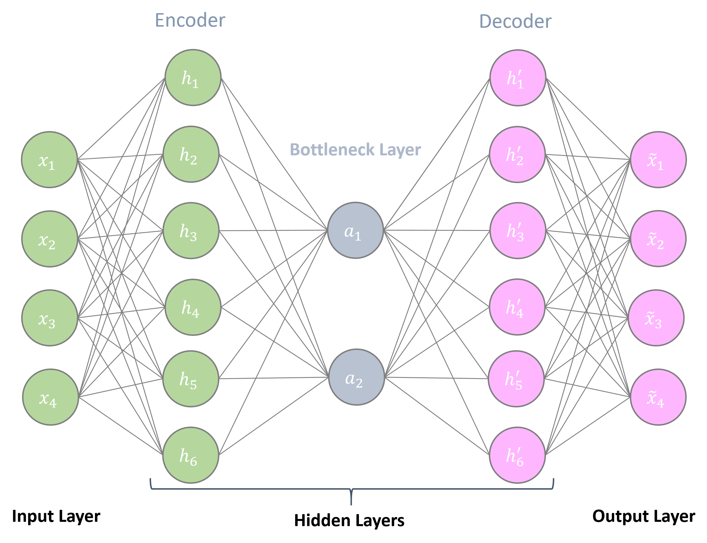
Autoencoders (AE)Kramer 1992 are a type of neural network designed for unsupervised learning tasks. The aim is usually to learn a new representation of the data, called an encoding. The AE is composed of two parts: the encoder learns the new representation and the decoder simultaneously learns to reconstruct the original data from this representation. The AE thus seeks to approximate the identity function. When the encoder is composed of one fully connected layer which reduces the dimension, together with a linear activation function, its learned representation is essentially the same as that of a PCA projection of the same dimensionality Plaut 2018; Bourlard and Kamp 1988: more precisely, the two models project on the same bottleneck space, but not using the same vectors. In general, however, AEs are used with nonlinear activation functions. This allows for nonlinear encoding functions, and thus potentially better encoders than those restricted to stay within the smaller class of linear functions.

AEs can have different topologies depending on the learning task, the data size and dimensionality, etc. Here, we describe the general autoencoder topology used in this work. We denote by $\mathcal{X}\subseteq\mathbb{R}^{D}$ the data space, and by $\mathcal{A}\subseteq\mathbb{R}^{d}$ a lower dimensional space ($d<D$). Figure 1 presents the typical topology of the AEs used in our work. The autoencoder can be represented by a mapping $f=f_{\text{dec}}\circ f_{\text{enc}}$ where $f_{\text{enc}}:\mathcal{X}\xrightarrow{}\mathcal{A}$, $f_{\text{dec}}:\mathcal{A}\xrightarrow{}\mathcal{X}$ and $\circ$ is the function composition operator i.e. $f_{\text{dec}}\circ f_{\text{enc}}(x)=f_{\text{dec}}\left(f_{\text{enc}}(x)\right)$. It is symmetrical in structure, fully connected, and contains $2L$ layers. Each hidden layer is of dimension $d_{\ell}=d_{2L-\ell}$ for $\ell=1\dots L$, and the output layer is of dimension $d_{2L}=D$ (Note that, by convention, the input layer does not count as a layer of the network). Each layer $\ell\in{1,\dots,2L}$ has an activation function $g_{\ell}$ and is connected to the previous layer by a projection matrix $W_{\ell}\in\mathbb{R}^{d_{\ell}\times d_{\ell-1}}$, and a bias vector $b_{\ell}\in\mathbb{R}^{d_{\ell}}$. There are thus $K=\displaystyle\sum_{\ell=1}^{L}d_{\ell}d_{\ell-1}+d_{\ell}$ learnable real parameters denoted by $(p_{1},\dots,p_{K})\in\mathbb{R}^{K}$. As the activation functions are predefined and do not change during learning, the autoencoder function is fully described by its parameters $\textbf{p}=(p_{k})_{k=1,\dots,K}$. We indicate this dependence as $f_{\textbf{p}}$. The general formula for $f_{\textbf{p}}$ is:

where the activation functions are by convention applied element-wise: for $z=(z_{1},\dots,z_{d_{\ell}})$, it holds that $g_{\ell}(z)=(g_{\ell}(z_{1}),\dots,g_{\ell}(z_{d_{\ell}}))$. Note that $f_{\textbf{p}}$, as well as $f_{\text{enc}}$, are differentiable functions when all the activation functions  $(g_{\ell})_{1\leq\ell\leq 2L}$ are.

There is a distinction to be made between the configurational space of the simulation, and the data space over which the learned model is optimized. Indeed, a preprocessing step is usually necessary to obtain a usable dataset from the sampled molecular trajectory. A notable example is the elimination of rotational and translational invariances through centering and structural alignment of the configurations to a reference structure, or by using internal coordinates (distances, angles, etc). Another example is using only a subset of the coordinates to reduce the data dimensionality, for example by taking out solvent molecules and hydrogen atoms, whose motions are often considered irrelevant. For the remainder of the paper, we denote by $q$ the configurations of the system, and by $x$ the corresponding post-processed data points. We however allow for an abuse of notation by keeping the same notation for various objects whose argument is either $q$ or $x$, depending on the context. For example, the probability measures $\mu(dq)$ and $\mu(dx)$ are denoted by the same symbol, even though $\mu(dx)$ is actually the image of $\mu(dq)$ by the application $q\mapsto x$.

Consider a probability distribution $\mu$ on $\mathcal{X}\subset\mathbb{R}^{D}$. Typically in MD, $\mu$ is the Boltzmann-Gibbs distribution and $\mathcal{X}$ is the configurational space of the system under study. We seek to encode configurations of $\mathcal{X}$ sampled from $\mu$ in a smaller dimensional space $\mathcal{A}\subset\mathbb{R}^{d}$, where $d<D$, using an autoencoder (AE). Theoretically, the optimal parameters $\textbf{p}_{\mu}$ minimize the expected loss

where the subscript $\mu$ in $\mathbb{E}_{\mu}$ indicates that $X$ is a random variable distributed according to $\mu$. We denote by $\textbf{p}_{\mu}$ a solution to the minimization of $\mathcal{L}(\mu,\textbf{p})$, provided it exists (which is always assumed here):

Note that $\textbf{p}_{\mu}$ is a priori not unique, and depends of course on the distribution $\mu$.

To accelerate the exploration of the phase space of the system under study, MD simulations can be biased to target another distribution than the Boltzmann-Gibbs reference measure. The resulting dataset is thus not drawn from the original distribution of interest $\mu$, but from a biased distribution $\widetilde{\mu}$. Since we want to optimize the loss (1), we need to reweight the configurations $x$ sampled from $\widetilde{\mu}$ by a factor

Note that to ensure that $w(x)$ is finite, we always assume that $\mu$ is absolutely continuous with respect to $\widetilde{\mu}$ (i.e. $\mu(A)=0$ for all measurable sets $A\subset\mathcal{X}$ such that $\widetilde{\mu}(A)=0$).

The reweighting corresponds to considering the loss function

Reweighting ensures that the same optimization problem as (2) is solved, even when the data points are not distributed according to $\mu$.

To approximate the expectation (5) with respect to $\widetilde{\mu}$, we again rely on an empirical weighted distribution:

The new discrete loss is thus a weighted average loss over the $\widetilde{\mu}$ sampled data:

which converges by the ergodic theorem almost surely to $\mathcal{L}(\mu,\textbf{p})$ when $N\xrightarrow{}\infty$.

Note that computing $(\widehat{w}_{i})_{1\leq i\leq N}$ only requires the knowledge of $\mu$ and $\widetilde{\mu}$ up to a multiplicative constant.

This section provides a 2D example for free energy biasing. This system is then used to illustrate the necessity of reweighting when training models over biased simulations. We use throughout the section some common definitions of free energy and Boltzmann–Gibbs density measure,recalled in Supp. Mat. Section A.1 for completeness.

Let us introduce the following three well potential, previously considered in other works Park et al. 2003:

In this example, the configurations $q$ are represented by the $2$ dimensional coordinates of the particle: $q=(x_{1},x_{2})$. The potential $V$ has two deep wells centered at $q_{\mathrm{L}}=(-1.113,-0.03685)$, $q_{\mathrm{R}}=(1.113,-0.03685)$, and a shallow well around $q_{\mathrm{C}}=(0,1.7566)$. We consider the overdamped Langevin dynamics:

where $B_{t}$ is a $2$-dimensional Brownian motion. The dynamics are discretized using the Euler–Maruyama scheme:

where $\{G^{j}\}_{j\geq 0}$ is a sequence of independent standard normal random vectors and $q^{j}\approx q_{j\Delta t}$. We simulate a sample trajectory of this system, with inverse temperature $\beta=4$ and time-step $\Delta t=10^{-3}$, starting from initial condition $q^{0}=(-1,0)$. Figure 2 gives a scatter plot of this trajectory as well as the time evolution of the coordinate $x_{1}$ .

The metastability of the dynamics is quite well characterized by the direction $x_{1}$, whereas $x_{2}$ is not enough to distinguish between the two deep wells. In the sequel, we consider $\xi_{1}(q)=x_{1}$ and $\xi_{2}(q)=x_{2}$ as two different choices of CV.

The free energies corresponding to the CVs $\xi_{1}$ and $\xi_{2}$ are respectively:

The quantities $F_{1}(x_{1})$ and $F_{2}(x_{2})$ can be easily approximated in this low dimensional example by a numerical quadrature. We can therefore easily sample from the three following probability measures: the unbiased Boltzmann-Gibbs probability distribution $\nu$ associated with the potential $V$, and the biased Boltzmann-Gibbs probability distributions $\nu_{F_{i}}$ associated with the biased potentials $V-F_{i}\circ\xi_{i}$ for $i=1,2$.

We now perform experiments to compare the results obtained from biased trajectories using different collective variables, with those from an unbiased trajectory. For this, we first simulate three trajectories. All three are long enough to sample the three potential wells of our system. The first trajectory is unbiased, following (10) with a timestep $\Delta t=10^{-3}$ for $N=4\times 10^{7}$ steps. Every $40$th configuration is kept as a datapoint. The second trajectory is free energy biased using $\xi_{1}(x_{1},x_{2})=x_{1}$ as CV, i.e., it follows (10) with potential $V-F_{1}\circ\xi_{1}$ instead of $V$, and a timestep $\Delta t=10^{-3}$ for $T=2\times 10^{6}$ steps. Configurations are saved every 2 timesteps. The third trajectory is free energy biased using $\xi_{2}(x_{1},x_{2})=x_{2}$ as a collective variable, and using the same simulation settings as the second trajectory. Note that the second and third trajectories are shorter: the duration of these trajectories were chosen so that they visit the full configurational space. These three trajectories serve as our training datasets. The datapoints are thus sampled respectively from the unbiased Boltzmann–Gibbs measure $\mu=\nu$, the free energy biased Boltzmann–Gibbs measure $\widetilde{\mu}_{1}=\nu_{F_{1}}$, and the free energy biased Boltzmann–Gibbs measure $\widetilde{\mu}_{2}=\nu_{F_{2}}$.

We next build five small autoencoders with the following topology: $D=2$ (input data dimensionality), $2L=2$ layers containing respectively $1$ and $2$ nodes, and $g_{1}(z)=\tanh(z)$ and $g_{2}(z)=z$, the identity function. The number of parameters is thus $K=7$ (including $3$ bias parameters). We use $\tanh$ as the bottleneck activation function in order to obtain a bounded learned collective variable with known bounds $[-1,1]$. All five autoencoders are initialized with the same random network parameters. We then separately train these autoencoders for a maximum of $200$ epochs each as follows:

• •

  The first AE is trained on the unbiased trajectory;

• •

  The second AE is trained on the $\xi_{1}$-biased trajectory;

• •

  The third AE is trained on the $\xi_{1}$-biased trajectory, but with reweighting, meaning that each data point $x^{i}=(x_{1}^{i},x_{2}^{i})$ contributes to the learning loss with

  $$\widehat{w}_{i}=N\frac{\mu(x^{i})/\widetilde{\mu}_{1}(x^{i})}{\displaystyle\sum_{j=1}^{N}\mu(x^{j})/\widetilde{\mu}_{1}(x^{j})}=N\displaystyle\frac{\mathrm{e}^{-\beta F_{1}(x^{i})}}{\displaystyle\sum_{j=1}^{N}\mathrm{e}^{-\beta F_{1}(x^{j})}}\text{ .}$$

• •

  The fourth AE is trained on the $\xi_{2}$-biased trajectory;

• •

  The fifth AE is trained on the $\xi_{2}$-biased trajectory, but reweighted using

  $$\widehat{w}_{i}=N\frac{\mu(x^{i})/\widetilde{\mu}_{2}(x^{i})}{\displaystyle\sum_{j=1}^{N}\mu(x^{j})/\widetilde{\mu}_{2}(x^{j})}=N\displaystyle\frac{\mathrm{e}^{-\beta F_{2}(x^{i})}}{\displaystyle\sum_{j=1}^{N}\mathrm{e}^{-\beta F_{2}(x^{j})}}\text{ .}$$

As discussed in Supp. Mat. Section A.4, the multiplication by the number of samples $N$ allows to comply with the default normalization of the weights of the ML package we use. A subset of the data is kept as validation set (here, $10\%$), and early stopping is applied when the validation loss no longer improves for $20$ consecutive epochs.

We compare the obtained encoders using heat maps. The values of the encoded bottleneck functions are computed over the (discretized) space $(x_{1},x_{2})\in[-2,2]\times[-1,2.5]$. The results are given in Figure 3. Note that the aim here is to compare encodings obtained from the different models, and possibly to have insight on how these encodings depend on the coordinates $x_{1}$ and $x_{2}$. Let us emphasize in particular that it is for example possible to obtain a function of $x_{1}$ instead of $x_{1}$ itself as encoder variable. For this reason, and to simplify the comparison between the obtained CVs, they are renormalized to have a range that is exactly between $0$ and $1$:

where $\xi_{\text{AE}}^{\min}$ and $\xi_{\text{AE}}^{\max}$ are respectively the minimum and maximum values taken by the encoder function $\xi_{\text{AE}}$ over the $2$-dimensional space $[-2,2]\times[-1,2.5]$. We draw two important conclusions upon interpreting the obtained results:

• •

  First, the encoding learned through unbiased training on the reference data obtained from a long unbiased trajectory (top panel) is a function of $x_{1}$, which we recall is considered a good CV as it distinguishes the three potential wells. The direction $x_{1}$ therefore corresponds to the target unbiased representation that we want to find using the remaining models (in particular with the reweighted learning). The encodings obtained from the reweighted training over the two biased trajectories (middle and bottom right panels) also represent bijective functions of $x_{1}$. The encodings obtained through biased unweighted learning, however, encode different variables (middle and bottom left panels). This is therefore an example where reweighting proves necessary for obtaining results that are consistent with unbiased learning.

• •

  It is interesting to note the difference between the CV obtained from biased learning over the $\xi_{1}$-trajectory (middle left panel) and the one obtained from the $\xi_{2}$-trajectory (bottom left panel). It is quite clear that the latter is closer to a monotonic function of the target learning result, $x_{1}$, than the former. These results can be intuitively explained as follows: Free energy biasing changes the distribution along the CV (here $\xi_{1}$ or $\xi_{2}$) to a uniform law, making the corresponding direction no longer relevant. This prompts the model to learn other directions that are still relevant in the biased simulation. In the case of the trajectory obtained by biasing with $F_{1}\circ\xi_{1}$, the $x_{1}$ direction is no longer a relevant feature of the data space and the encoder does not recover it. On the other hand, biasing using $F_{2}\circ\xi_{2}$ does not completely annihilate the relevance of the variable $x_{1}$ in the sampled data. This explains why the CV learned from biasing with $\xi_{2}$ is closer to $x_{1}$.

This last point is very important as it means that if an iterative learning run is performed without reweighting, then whenever a good CV is learned at iteration $n$, this CV may be cancelled out in the next iteration, making convergence difficult to achieve.

This section provides a description of the steps of our iterative algorithm, which we call FEBILAE, for "Free Energy Biasing and Iterative Learning with AutoEncoders". The algorithm is also summarized in the pseudo-code of Algorithm 1.

With the exception of low dimensional systems ($D\leq 3$) such as the example used in Section 2.5, the free energy of a system associated with a given CV cannot be easily estimated. Adaptive sampling algorithms replace the actual free energy $F$ by an estimated function $F_{t}$ in the biased dynamics at time $t$, meaning that the potential becomes $V-F_{t}\circ\xi$. The estimate $F_{t}$ is updated on-the-fly so that it converges to $F$ as the molecular dynamics simulation proceeds. The two categories of adaptive biasing techniques are Lelièvre et al. 2007 Adaptive Biasing Potential (ABP) methods, where the free energy $F_{t}$ is estimated and its gradient, the so-called mean force, is then used in the dynamics; and Adaptive Biasing Force (ABF) methods where the mean force is estimated directly, and the free energy is subsequently obtained by numerical integration through a Helmholtz projection Alrachid and Lelièvre 2015.

In this work, we choose to work with ABF, and more precisely extended system ABF (eABF) Lesage et al. 2016 for free energy biasing. We call this version of the algorithm AE-ABF. Section 3.2.1 gives a brief description of ABF. We then recall its main limitation, namely that it requires the computation of the second order derivatives of the used CVs. This motivates using eABF, which is described in Section 3.2.2.

This section discusses two ways of using part of the information learned in previous iterations to possibly improve or accelerate the learning or sampling in the next iteration. Following the notation in Algorithm 1, the iteration index is denoted by $i$.

In order to illustrate the methodology developed in this section, we come back to the 2 dimensional example introduced in Section 2.5, with the same parameters as in this section unless otherwise specified. For this toy example, the routines for unbiased simulations as well as eABF simulations were implemented in python using the numpy module.

We demonstrate on this simple 2D example that reweighting the sampled configurations leads to a fast convergence to the CV $\xi_{1}(x)=x_{1}$ (which is the CV obtained by training on a long unbiased trajectory), whereas not reweighting can lead the algorithm to be trapped, continually learning different CVs between consecutive iterations. We start with the initial unbiased simulation, which is purposedly stopped before it crosses the first energy barrier: The trajectory is simulated starting from the initial condition $q^{0}=(-1,0)$, for $2\times 10^{7}$ timesteps, with $\Delta t=10^{-3}$, keeping $1$ out of $50$ datapoints. The time horizon of the simulation is thus $T=2\times 10^{4}$, and the dataset contains $N=4\times 10^{5}$ samples belonging to only one metastable state.

We then use this dataset to start two separate learning frameworks. The first one uses reweighting at each iteration as discussed in Section 3.1. The second one does not use reweighting before achieving a new round of training (i.e. the weights $\widehat{w}_{j}$ in (7) are all set to $1$). All autoencoders are initialized with the same parameters at each iteration, and are trained using $80\%$ of the data for training (and $20\%$ for validation), with batch size $b=400$, and $N/b=8\times 10^{2}$ steps per epoch for a maximum of $100$ epochs with early stopping when the validation loss does not improve for $20$ consecutive epochs. At each new iteration, for both schemes, eABF is performed for $1.2\times 10^{6}$ timesteps with $\Delta t=10^{-3}$, and $1$ in every $3$ configurations are kept. The time horizon of the simulation is thus $T=1.2\times 10^{3}$ and the datasets all contain $N=4\times 10^{5}$ samples. eABF is run with a force constant $\kappa=50$. Note again that the biased simulations have a smaller time horizon than the unbiased simulation, since biasing accelerates the exploration of all states of the configurational space. The CV intervals are determined using the range $[z_{\min},z_{\max}]$ of the values the CV takes over the training data. Regardless of the chosen CV interval, we use a grid of $200$ bins to discretize the CV. Each simulation is started at the same point $(x_{1},x_{2})=(-1,0)$. The estimated mean force over a certain bin is only applied after 100 samples are collected inside this bin. Finally, the CV gradients needed for ABF are extracted from the autoencoders using keras functions.

Figure 4 illustrates heat maps of the encodings obtained at each iteration for both schemes. All CVs were renormalized using Equation (12) to have a range within $[0,1]$. As shown in Figure 4 left, after only two iterations, the reweighted model finds the CV $x_{1}$ and stabilizes. The biased model, on the other hand, learns a different direction at each new iteration, so that the learned CV does not converge, but rather seems to oscillate between two different functions.

We use the keras Chollet 2015 library to wrap the tensorflow Abadi et al. 2015 neural network module in python.

In order to construct an entirely automated code, all molecular simulations were performed with the openmm software Eastman et al. 2017 within its python API. The adaptive biasing and collective variable analysis were mainly performed using plumed Bonomi et al. 2019; Tribello et al. 2014; Chen et al. 2018. To link these two modules, we used the openmmplumed plugin module omm. Additionally, the colvar Fiorin et al. 2013 abf integrate utility was used to recover the potential of mean force from the gradients computed by eABF.

Our goal is to have an implementation that is automated and entirely runnable from python. Consequently, our implementation is practical and easy to use, but not necessarily computationally optimized.

Chignolin, a 10-residue miniprotein with a beta-hairpin structure, is another well-studied system, particularly for its distinct folding states captured using MD at accessible timescales Lindorff-Larsen et al. 2011; Satoh et al. 2006. Lacking an X-ray for the wild-type form, herein, we use the CLN025 mutant (PDB ID: 5AWL) in explicit solvent as a more realistic and challenging system of our approach. After the addition of hydrogen atoms, the system contains $166$ atoms.

Conventionally the 2D intrinsic manifold of alanine dipeptide in vacuum is described by the $\Phi$ and $\Psi$ backbone dihedrals Bolhuis et al. 2000; Hashemian and Arroyo 2015. As mentioned in Remark 1, we have used the plateau method to check that the bottleneck optimal dimensionality is indeed $d=2$. See Supp. Mat. Section D where we provide the FVE curve computed using a long unbiased trajectory of alanine dipeptide.

We first present in Section 5.1.1 the ground truth CV, which is the CV obtained from training an autoencoder over a long unbiased simulation. The quality of this CV is assessed by measuring its ability to recover the free energy landscape of the dihedral angles $\Phi,\Psi$. Section 5.1.2 contains the results of applying AE-ABF to alanine dipeptide. For a concise presentation of this toy system, see Supp. Mat. Section D.

References

- Shaw et al. (2010) Shaw, D.; Maragakis, P.; Lindorff-Larsen, K.; Piana, S.; Dror, R.; Eastwood, M.; Bank, J.; Jumper, J.; Salmon, J.; Shan, Y.; Wriggers, W. Science 2010, 330, 341–346.
- Hollingsworth and Dror (2018) Hollingsworth, S.; Dror, R. Neuron 2018, 99, 1129–1143.
- Hashemian et al. (2013) Hashemian, B.; Millán, D.; Arroyo, M. Journal of Chemical Physics 2013, 139, 214101.
- Abrams and Bussi (2014) Abrams, C.; Bussi, G. Entropy 2014, 16, 163–199.
- Marinari and Parisi (1992) Marinari, E.; Parisi, G. Europhysics Letters 1992, 19, 451.
- Swendsen and Wang (1986) Swendsen, R.; Wang, J. Physical Review Letters 1986, 57, 2607.
- Rhee and Pande (2003) Rhee, Y.; Pande, V. Biophysical Journal 2003, 84, 775–786.
- Nakajima et al. (1997) Nakajima, N.; Nakamura, H.; Kidera, A. Journal of Physical Chemistry B 1997, 101, 817–824.
- Sørensen and Voter (2000) Sørensen, M.; Voter, A. Journal of Chemical Physics 2000, 112, 9599–9606.
- Wang and Landau (2001) Wang, F.; Landau, D. Physical Review Letters 2001, 86, 2050.
- Laio and Gervasio (2008) Laio, A.; Gervasio, F. Reports on Progress in Physics 2008, 71, 126601.
- Laio and Parrinello (2002) Laio, A.; Parrinello, M. Proceedings of the National Academy of Sciences 2002, 99, 12562–12566.
- Kästner (2011) Kästner, J. Wiley Interdisciplinary Reviews: Computational Molecular Science 2011, 1, 932–942.
- Torrie and Valleau (1977) Torrie, G.; Valleau, J. Journal of Computational Physics 1977, 23, 187–199.
- Comer et al. (2015) Comer, J.; Gumbart, J.; Hénin, J.; Lelièvre, T.; Pohorille, A.; Chipot, C. Journal of Physical Chemistry B 2015, 119, 1129–1151.
- Hénin and Chipot (2004) Hénin, J.; Chipot, C. Journal of Chemical Physics 2004, 121, 2904–2914.
- Darve and Pohorille (2001) Darve, E.; Pohorille, A. Journal of Chemical Physics 2001, 115, 9169–9183.
- Mironov et al. (2019) Mironov, V.; Alexeev, Y.; Mulligan, V.; Fedorov, D. Journal of Computational Chemistry 2019, 40, 297–309.
- Ma and Dinner (2005) Ma, A.; Dinner, A. Journal of Physical Chemistry B 2005, 109, 6769–6779.
- Gkeka et al. (2020) Gkeka, P.; Stoltz, G.; Barati Farimani, A.; Belkacemi, Z.; Ceriotti, M.; Chodera, J.; Dinner, A.; Ferguson, A.; Maillet, J.; Minoux, H.; Peter, C.; Pietrucci, F.; Silveira, A.; Tkatchenko, A.; Trstanova, Z.; Wiewiora, R.; Lelièvre, T. Journal of Chemical Theory and Computation 2020, 16, 4757–4775.
- Glielmo et al. (2021) Glielmo, A.; Husic, B.; Rodriguez, A.; Clementi, C.; Noé, F.; Laio, A. Chemical Reviews 2021,
- Sidky et al. (2020) Sidky, H.; Chen, W.; Ferguson, A. Molecular Physics 2020, 118, e1737742.
- Nüske et al. (2014) Nüske, F.; Keller, B.; Pérez-Hernández, G.; Mey, A.; Noé, F. Journal of Chemical Theory and Computation 2014, 10, 1739–1752.
- Klus et al. (2018) Klus, S.; Nüske, F.; Koltai, P.; Wu, H.; Kevrekidis, I.; Schütte, C.; Noé, F. Journal of Nonlinear Science 2018, 28, 985–1010.
- Wu et al. (2017) Wu, H.; Nüske, F.; Paul, F.; Klus, S.; Koltai, P.; Noé, F. Journal of Chemical Physics 2017, 146, 154104.
- Coifman et al. (2008) Coifman, R.; Kevrekidis, I.; Lafon, S.; Maggioni, M.; Nadler, B. Multiscale Modeling & Simulation 2008, 7, 842–864.
- Nadler et al. (2006) Nadler, B.; Lafon, S.; Coifman, R.; Kevrekidis, I. Applied and Computational Harmonic Analysis 2006, 21, 113–127.
- Husic and Pande (2018) Husic, B.; Pande, V. Journal of the American Chemical Society 2018, 140, 2386–2396.
- Chodera and Noé (2014) Chodera, J.; Noé, F. Current Opinion in Structural Biology 2014, 25, 135–144.
- Molgedey and Schuster (1994) Molgedey, L.; Schuster, H. Physical Review Letters 1994, 72, 3634.
- Mardt et al. (2018) Mardt, A.; Pasquali, L.; Wu, H.; Noé, F. Nature Communications 2018, 9, 1–11.
- Chen et al. (2019) Chen, W.; Sidky, H.; Ferguson, A. Journal of Chemical Physics 2019, 150, 214114.
- Sultan and Pande (2018) Sultan, M.; Pande, V. Journal of Chemical Physics 2018, 149, 094–106.
- Sultan et al. (2014) Sultan, M.; Kiss, G.; Shukla, D.; Pande, V. Journal of Chemical Theory and Computation 2014, 10, 5217–5223.
- Peters and Trout (2006) Peters, B.; Trout, B. Journal of Chemical Physics 2006, 125, 054108.
- Rogal et al. (2019) Rogal, J.; Schneider, E.; Tuckerman, M. Physical Review Letters 2019, 123, 245701.
- Bonati et al. (2020) Bonati, L.; Rizzi, V.; Parrinello, M. Journal of Physical Chemistry Letters 2020, 11, 2998–3004.
- Kramer (1992) Kramer, M. Computers & Chemical Engineering 1992, 16, 313–328.
- Wehmeyer and Noé (2018) Wehmeyer, C.; Noé, F. Journal of Chemical Physics 2018, 148, 241703.
- Schöberl et al. (2019) Schöberl, M.; Zabaras, N.; Koutsourelakis, P.-S. Journal of Chemical Physics 2019, 150, 024109.
- Kingma and Welling (2013) Kingma, D.; Welling, M. arXiv preprint arXiv:1312.6114 2013,
- Hernández et al. (2018) Hernández, C.; Wayment-Steele, H.; Sultan, M.; Husic, B.; Pande, V. Physical Review E 2018, 97, 062412.
- Varolgüneş et al. (2020) Varolgüneş, Y. B.; Bereau, T.; Rudzinski, J. Machine Learning: Science and Technology 2020, 1, 015012.
- Frassek et al. (2021) Frassek, M.; Arjun, A.; Bolhuis, P. Journal of Chemical Physics 2021, 155, 064103.
- Felsberger and Koutsourelakis (2018) Felsberger, L.; Koutsourelakis, P.-S. arXiv preprint arXiv:1802.03824 2018,
- Ravindra et al. (2020) Ravindra, P.; Smith, Z.; Tiwary, P. Molecular Systems Design & Engineering 2020, 5, 339–348.
- Chen and Ferguson (2018) Chen, W.; Ferguson, A. Journal of Computational Chemistry 2018, 39, 2079–2102.
- Chen et al. (2018) Chen, W.; Tan, A.; Ferguson, A. Journal of Chemical Physics 2018, 149, 072–312.
- Ribeiro et al. (2018) Ribeiro, J.; Bravo, P.; Wang, Y.; Tiwary, P. Journal of Chemical Physics 2018, 149, 072301.
- Wang et al. (2019) Wang, Y.; Ribeiro, J. M. L.; Tiwary, P. Nature communications 2019, 10, 1–8.
- Plaut (2018) Plaut, E. arXiv preprint arXiv:1804.10253 2018,
- Bourlard and Kamp (1988) Bourlard, H.; Kamp, Y. Biological Cybernetics 1988, 59, 291–294.
- Park et al. (2003) Park, S.; Sener, M.; Lu, D.; Schulten, K. Journal of Chemical Physics 2003, 119, 1313–1319.
- Lelièvre et al. (2007) Lelièvre, T.; Rousset, M.; Stoltz, G. Journal of Chemical Physics 2007, 126, 134111.
- Alrachid and Lelièvre (2015) Alrachid, H.; Lelièvre, T. The SMAI Journal of Computational Mathematics 2015, 1, 55–82.
- Lesage et al. (2016) Lesage, A.; Lelièvre, T.; Stoltz, G.; Hénin, J. Journal of Physical Chemistry B 2016, 121, 3676–3685.
- Lelièvre et al. (2010) Lelièvre, T.; Rousset, M.; Stoltz, G. Free-energy Computations: A Mathematical Perspective; Imperial College Press, 2010.
- Chollet (2015) Chollet, F. Keras. 2015; https://github.com/fchollet/keras.
- Abadi et al. (2015) Abadi, M.; Agarwal, A.; Barham, P.; Brevdo, E.; Zhifeng Chen, Z.; Citro, C.; Corrado, G.; Davis, A.; Dean, J.; Devin, M.; Ghemawat, S.; Goodfellow, I.; Harp, A.; Irving, G.; Isard, M.; Jia, Y.; Jozefowicz, R.; Kaiser, L.; Kudlur, M.; Levenberg, J.; Mané, D.; Monga, R.; Moore, S.; Murray, D.; Ola, C.; Schuster, M.; Shlens, J.; Steiner, B.; Sutskever, I.; Talwar, K.; Tucker, P.; Vanhoucke, V.; Vasudevan, V.; Viégas, F.; Vinyals, O.; Warden, P.; Wattenberg, M.; Wicke, M.; Yu, Y.; Zheng, X. TensorFlow: Large-scale machine learning on heterogeneous systems. 2015; http://tensorflow.org/, Software available from tensorflow.org.
- Eastman et al. (2017) Eastman, P.; Swails, J.; Chodera, J.; McGibbon, R.; Zhao, Y.; Beauchamp, K.; Wang, L.; Simmonett, A.; Harrigan, M.; Stern, C.; Wiewiora, R.; Brooks, B.; Pande, V. PLOS Computational Biology 2017, 13, 1–17.
- Bonomi et al. (2019) Bonomi, M.; Bussi, G.; Camilloni, C.; Tribello, G.; Banáš, P.; Barducci, A.; Bernetti, M.; Bolhuis, P.; Bottaro, S.; Branduardi, D. Nature Methods 2019, 16, 670–673.
- Tribello et al. (2014) Tribello, G.; Bonomi, M.; Branduardi, D.; Camilloni, C.; Bussi, G. Computer Physics Communications 2014, 185, 604–613.
- Chen et al. (2018) Chen, H.; Fu, H.; Shao, X.; Chipot, C.; Cai, W. Journal of chemical information and modeling 2018, 58, 1315–1318.
- (64) openmm-plumed: OpenMM plugin to interface with Plumed. https://github.com/openmm/openmm-plumed.
- Fiorin et al. (2013) Fiorin, G.; Klein, M.; Hénin, J. Molecular Physics 2013, 111, 3345–3362.
- Kabsch (1978) Kabsch, W. Acta Crystallographica Section A 1978, 34, 827–828.
- Kingma and Ba (2014) Kingma, D.; Ba, J. 3rd International Conference for Learning Representations 2014,
- Morgan and Bourlard (1990) Morgan, N.; Bourlard, H. In Advances in Neural Information Processing Systems 2; Touretzky, D. S., Ed.; Morgan-Kaufmann, 1990; pp 630–637.
- Hornak et al. (2006) Hornak, V.; Abel, R.; Okur, A.; Strockbine, B.; Roitberg, A.; Simmerling, C. Proteins: Structure, Function, and Bioinformatics 2006, 65, 712–725.
- Lindorff-Larsen et al. (2011) Lindorff-Larsen, K.; Piana, S.; Dror, R.; Shaw, D. Science 2011, 334, 517–520.
- Satoh et al. (2006) Satoh, D.; Shimizu, K.; Nakamura, S.; Terada, T. FEBS Letters 2006, 580, 3422–3426.
- Lindorff-Larsen et al. (2010) Lindorff-Larsen, K.; Piana, S.; Palmo, K.; Maragakis, P.; Klepeis, J.; Dror, R.; Shaw, D. Proteins: Structure, Function, and Bioinformatics 2010, 78, 1950–1958.
- Jorgensen et al. (1983) Jorgensen, W.; Chandrasekhar, J.; Madura, J.; Impey, R.; Klein, M. Journal of Chemical Physics 1983, 79, 926–935.
- Hess et al. (1997) Hess, B.; Bekker, H.; Berendsen, H.; Fraaije, J. Journal of Computational Chemistry 1997, 18, 1463–1472.
- Bolhuis et al. (2000) Bolhuis, P.; Dellago, C.; Chandler, D. Proceedings of the National Academy of Sciences 2000, 97, 5877–5882.
- Hashemian and Arroyo (2015) Hashemian, B.; Arroyo, M. Journal of Chemical Physics 2015, 142, 044102.
- Honda et al. (2004) Honda, S.; Yamasaki, K.; Sawada, Y.; Morii, H. Structure 2004, 12, 1507–1518.
Appendix A Theoretical definitions and practical details
This section highlights some important theoretical and practical points on the implementation of FEBILAE.
A.1 Collective variables and free energy biasing
In MD, a common choice for the biased distribution is to consider a free energy biased distribution. In order to make this concept precise, we recall in this section some definitions on collective variables, free energy and free energy based biasing, including general formulas for the Boltzmann–Gibbs measure and the free energy biased measure. Here, we consider the positions of a given system , where for systems in vacuum or in the case of periodic boundary conditions in a cubic box. We denote by the dimensionality of the system. For this system, the marginal of the canonical measure with respect to the positions is defined as: