跳到论文正文
W Papers独立论文阅读器 arXiv:2104.11007 论文正文 计算阅读时间 · 0%
引用这篇论文根据当前论文元数据生成,正式投稿前建议核对。


License: CC Zero
arXiv:2104.11007v1 [math-ph] 22 Apr 2021

Breakdown of superconductivity in a magnetic field with self-intersecting zero set

and Kamel Attar
Abstract.

We prove that the lowest eigenvalue of the Laplace operator with a magnetic field having a self-intersecting zero set is a monotone function of the parameter defining the strength of the magnetic field, in a neighborhood of infinity. We apply this monotonicity result on the study of the transition from superconducting to normal states for the Ginzburg-Landau model, and prove that the transition occurs at a unique threshold value of the applied magnetic field.

1. Introduction

1.1. Breakdown of superconductivity.

Superconductivity is a state of metals and alloys that appear below a certain critical temperature Tc\displaystyle T_{c}. When the temperature is below Tc\displaystyle T_{c} the body must be in the superconducting state; if an applied magnetic field (with small intensity) attempts to destroy the superconductivity, an induced magnetic field appears and repels the applied magnetic field. If the intensity of the applied magnetic field is increased gradually past a critical value, the superconductor can no longer resist the magnetic field and the appearance of superconductivity in the metal decreases gradually past critical conducting states (superconducting state, mixed conducting state and normal conducting state). Eventually, a large magnetic field destroys superconductivity from the sample (see Figure 1).

Refer to caption
Figure 1. Schematic representation of a material shows the difference states.

In the case of a uniform applied magnetic field, phase transitions associated with a type II superconductor are marked by three thresholds:

  • •

    HC1\displaystyle H_{C_{1}} is the intensity of the magnetic field where a superconductor switches from the superconducting state to the mixed conducting state (vortex state). In this case the superconductor allows the applied magnetic field to pass through small regions of the sample [31].

  • •

    HC2\displaystyle H_{C_{2}} is the intensity of the magnetic field that corresponds to the transition from superconductivity located in regions far from the boundary to surface superconductivity [29, 32, 15].

  • •

    HC3\displaystyle H_{C_{3}} is the intensity of the magnetic field that corresponds to the transition from surface superconductivity to the normal conducting state; in this case the superconductivity can no longer exist in the superconductor [29, 10, 7].

Non uniform magnetic fields is the subject of recent research:

  • •

    Non-vanishing smooth magnetic fields [10, 30, 25] ;

  • •

    Sign-changing smooth magnetic fields [28, 18] ;

  • •

    Non-smooth magnetic fields [1, 3, 23] .

In this contribution, we study smooth magnetic fields with a self-intersecting zero set.

1.2. Magnetic field with self-intersecting zeros

Suppose that Ω⊂ℝ2\displaystyle\Omega\subset\mathbb{R}^{2} is bounded, open, simply connected with smooth boundary. Consider a vertical magnetic field of the form

B0​z→B_{0}\vec{z}

where the function B0∈C∞​(Ω¯)\displaystyle B_{0}\in C^{\infty}(\overline{\Omega}) has a non-trivial zero set

(1.1) Γ={x∈Ω¯:B0​(x)=0}andΣ={x∈Γ:∇B0​(x)=0}\Gamma=\{x\in\overline{\Omega}:B_{0}(x)=0\}\qquad\text{and}\qquad\Sigma=\{x\in\Gamma:\nabla B_{0}(x)=0\}

and satisfies the following properties (see [8])

Γ≠∅,Σ≠∅​is​finite,Σ∩∂Ω=∅\Gamma\neq\varnothing,\quad\Sigma\neq\varnothing{\rm\penalty\ is\penalty\ finite,}\quad\Sigma\cap\partial\Omega=\varnothing

and

(1.2) {|B0|+|∇B0|>0 in ​Ω¯∖Σ(a)∇B0×n→≠0 on ​Γ∩∂Ω(b)|∇B0|+|Hess​B0|>0 on ​Γ(c)τ1→×τ2→≠0 on ​Σ(d).\left\{\begin{array}[]{rll}|B_{0}|+|\nabla B_{0}|>0&\mbox{ in }\overline{\Omega}\setminus\Sigma&(a)\\ \nabla B_{0}\times\vec{n}\neq 0&\mbox{ on }\Gamma\cap\partial\Omega&(b)\\ |\nabla B_{0}|+|{\rm Hess}B_{0}|>0&\mbox{ on }\Gamma&(c)\\ \vec{\tau_{1}}\times\vec{\tau_{2}}\neq 0&\mbox{ on }\Sigma&(d)\,.\end{array}\right.

Here n→\displaystyle\vec{n} is the unit normal vector to the boundary, τ→1\displaystyle\vec{\tau}_{1} and τ→2\displaystyle\vec{\tau}_{2} are the unit tangent vector on the intersection point x∈Σ\displaystyle x\in\Sigma, and Hess​B0\displaystyle{\rm Hess}B_{0} is the Hessian matrix of the magnetic field at the point x\displaystyle x which has two non-zero eigenvalues λ1Hess​(x)\displaystyle\lambda^{\rm Hess}_{1}(x) and λ2Hess​(x)\displaystyle\lambda^{\rm Hess}_{2}(x) with opposite signs and labeled as follows

(1.3) |λ1Hess​(x)|≤|λ2Hess​(x)|(x∈Σ).|\lambda^{\rm Hess}_{1}(x)|\leq|\lambda^{\rm Hess}_{2}(x)|\quad(x\in\Sigma)\,.

Assumption (1.2)(a)\displaystyle\eqref{B(x)}_{(a)} implies that for any open set ω\displaystyle\omega relatively compact in Ω\displaystyle\Omega, Γ∩ω\displaystyle\Gamma\cap\omega is either empty, or consists of a union of smooth curves and the quantity |∇B0|\displaystyle|\nabla B_{0}| does not vanish on Γ\displaystyle\Gamma. We see from (1.2)(b)\displaystyle\eqref{B(x)}_{(b)} that the B0\displaystyle B_{0} is allowed to vanish on a finite number of boundary points and that the curve Γ\displaystyle\Gamma cannot intersect tangentially ∂Ω\displaystyle\partial\Omega. Assumptions (1.2)(c)\displaystyle\eqref{B(x)}_{(c)} and (1.2)(d)\displaystyle\eqref{B(x)}_{(d)} tell us that the smooth curves can intersect on isolated points where |∇B0|\displaystyle|\nabla B_{0}| vanishes.

The case where the magnetic field vanishes non-degenerately along a smooth non self intersecting curve, is the subject of numerous works in the contexts of shape optimization[27], superconductivity [28, 18, 2] and semiclassical spectral asymptotics [9, 6].

Refer to caption
Figure 2. Schematic representation of a domain subject to a variable magnetic field that vanishes along the curve Γ\displaystyle\Gamma which crosses itself inside the domain.

1.3. Magnetic Laplacian and strong diamagnetism

Consider the unique vector field 𝐅∈H1​(Ω,ℝ2)\displaystyle\mathbf{F}\in H^{1}(\Omega;\mathbb{R}^{2}) satisfying the following properties

(1.4) ν⋅𝐅=0​on​∂Ω,div​𝐅=0&curl⁡𝐅=B0​in​Ω,\nu\cdot\mathbf{F}=0\penalty\ {\rm on\penalty\ }\partial\Omega,\quad{\rm div}\mathbf{F}=0\penalty\ \&\penalty\ \curl\mathbf{F}=B_{0}{\penalty\ \rm in\penalty\ }\Omega\,,

where ν\displaystyle\nu is the unit outward normal of the boundary of Ω\displaystyle\Omega.

Let us introduce the magnetic Schrödinger operator

(1.5) Pb​𝐅Ω=−(∇−i​b​𝐅)2,P_{b\mathbf{F}}^{\Omega}=-(\nabla-ib\mathbf{F})^{2}\,,

with domain

D⁡(Pb​𝐅Ω):={u∈𝒱⁡(Ω):Pb​𝐅Ω​u∈L2​(Ω)&ν⋅(∇−i​b​𝐅)​u=0​on​∂Ω}.D(P_{b\mathbf{F}}^{\Omega}):=\{u\in\mathcal{V}(\Omega)\penalty\ :\penalty\ P_{b\mathbf{F}}^{\Omega}u\in L^{2}(\Omega)\penalty\ \&\penalty\ \nu\cdot(\nabla-ib\mathbf{F})u=0\penalty\ {\rm on}\penalty\ \partial\Omega\}\,.

The lowest eigenvalue (ground state energy) of this operator is

(1.6) μ1​(b​𝐅)=infϕ∈H1​(Ω)ϕ≠0(𝒬b​𝐅Ω​(ϕ)‖ϕ‖L2​(Ω)2),\mu_{1}(b\mathbf{F})=\inf_{\begin{subarray}{c}\phi\in H^{1}(\Omega)\\ \phi\neq 0\end{subarray}}\left(\frac{\mathcal{Q}_{b\mathbf{F}}^{\Omega}(\phi)}{\|\phi\|^{2}_{L^{2}(\Omega)}}\right)\,,

where

(1.7) 𝒬b​𝐅Ω​(ϕ)=∫Ω|(∇−i​b​𝐅)​ϕ|2​𝑑x.\mathcal{Q}_{b\mathbf{F}}^{\Omega}(\phi)=\int_{\Omega}|(\nabla-ib\mathbf{F})\phi|^{2}\,dx\,.

The large field limit b→+∞\displaystyle b\to+\infty can be transformed to a semi-classical limit by introducing the small parameter h=1b\displaystyle h=\frac{1}{b}. The full asymptotic expansion of the lowest eigenvalue Pb​𝐅Ω\displaystyle P_{b\mathbf{F}}^{\Omega} is derived by Dauge, Miqueu and Raymond [8]. Based on it, we prove the monotonicity of μ1​(b​𝐅)\displaystyle\mu_{1}(b\mathbf{F}) with respect to b\displaystyle b in a neighborhood of +∞\displaystyle+\infty. This property is named strong diamagnetism in the literature [10, 11, 12].

Theorem 1.1.

There exists b0>0\displaystyle b_{0}>0, such that the function b⟼μ1​(b​𝐅)\displaystyle b\longmapsto\mu_{1}(b\mathbf{F}) is monotone increasing on [b0,+∞[\displaystyle[b_{0},+\infty[.

Strong diamagnetism has been proved earlier under different assumptions on Ω\displaystyle\Omega and B0\displaystyle B_{0} [11, 5, 4]. Counterexamples of strong diamagnetism do exist [16, 19, 21, 22].

1.4. Ginzburg-Landau model

Consider the Ginzburg-Landau functional

(1.8) ℰκ,H,B0​(ψ,𝐀)=∫Ω(|(∇−i​κ​H​𝐀)​ψ|2+κ22​(1−|ψ|2)2)​𝑑x+κ2​H2​∫Ω|curl⁡𝐀−B0|2​𝑑x.\mathcal{E}_{\kappa,H,B_{0}}(\psi,\mathbf{A})=\int_{\Omega}\left(|(\nabla-i\kappa H\mathbf{A})\psi|^{2}+\frac{\kappa^{2}}{2}(1-|\psi|^{2})^{2}\right)\,dx+\kappa^{2}H^{2}\int_{\Omega}|\curl\mathbf{A}-B_{0}|^{2}\,dx\,.

The vector field 𝐀\displaystyle\mathbf{A} is called the magnetic potential which describes the induced magnetic field in the sample via

curl⁡𝐀=∇→×𝐀.\curl\mathbf{A}=\overrightarrow{\nabla}\times\mathbf{A}\,.

The positive number κ\displaystyle\kappa is the characteristic scale of the superconductor that distinguishes the material of the sample; we will study the case of materials of type II where κ\displaystyle\kappa is sufficiently large (κ→∞\displaystyle\kappa\to\infty). The complex-valued function ψ\displaystyle\psi is the order parameter that rises in the superconductor phase, where the modulus squared |ψ⁡(x)|2\displaystyle|\psi(x)|^{2} can be interpreted as the local density of the superconducting electron Cooper pairs as follows:

  • •

    If |ψ⁡(x)|≠0\displaystyle|\psi(x)|\neq 0, then at location x\displaystyle x, the material is in the superconducting state.

  • •

    If |ψ⁡(x)|=0\displaystyle|\psi(x)|=0, then at location x\displaystyle x, there exists no Cooper pairs, and the material is in the normal state.

  • •

    If |ψ⁡(x)|\displaystyle|\psi(x)| has zeros but does not vanish identically, the material is in the mixed state.

Since the functional is invariant under gauge transformations (ψ,𝐀)→(ei​κ​H​χ​ψ,𝐀−∇χ)\displaystyle(\psi,\mathbf{A})\to(e^{i\kappa H\chi}\psi,\mathbf{A}-\nabla\chi), it is enough to consider configurations (ψ,𝐀)\displaystyle(\psi,\mathbf{A}) in the space H1​(Ω,ℂ)×Hdiv1​(Ω)\displaystyle H^{1}(\Omega;\mathbb{C})\times H^{1}_{\Div}(\Omega) of sobolev functions, where

(1.9) Hdiv1(Ω)={𝐀=(𝐀1,𝐀2)∈H1(Ω)×H1(Ω):div𝐀=0inΩ,𝐀⋅ν=0on∂Ω},H^{1}_{\Div}(\Omega)=\Big\{\mathbf{A}=(\mathbf{A}_{1},\mathbf{A}_{2})\in H^{1}(\Omega)\times H^{1}(\Omega)\penalty\ :\penalty\ \Div\mathbf{A}=0\penalty\ {\rm in}\penalty\ \Omega\,,\,\mathbf{A}\cdot\nu=0\penalty\ {\rm on}\,\partial\Omega\,\Big\}\,,

with ν\displaystyle\nu being the unit interior normal vector of ∂Ω\displaystyle\partial\Omega.

The equilibrium state of the system will be where the total energy ℰκ,H,B0\displaystyle\mathcal{E}_{\kappa,H,B_{0}} is minimal, we denote by (ψ,𝐀)\displaystyle(\psi,\mathbf{A}) the minimizing configuration of ℰκ,H,B0\displaystyle\mathcal{E}_{\kappa,H,B_{0}}. When ψ=0\displaystyle\psi=0, the minimizing configuration is in the form (0,𝐅)\displaystyle(0,\mathbf{F}) with 𝐅\displaystyle\mathbf{F} in Hdiv1​(Ω)\displaystyle H^{1}_{\Div}(\Omega) such that curl⁡𝐅=B0\displaystyle\curl\mathbf{F}=B_{0}. Notice that this solution is unique (up to a gauge transformation) and we call the pair (0,𝐅)\displaystyle(0,\mathbf{F}) the normal state.

Ginzburg-Landau equations

Minimizers, (ψ,𝐀)∈H1​(Ω,ℂ)×Hdiv1​(Ω)\displaystyle(\psi,\mathbf{A})\in H^{1}(\Omega;\mathbb{C})\times H^{1}_{\Div}(\Omega) of (1.8) have to satisfy the Ginzburg-Landau equations,

(1.10) {−(∇−i​κ​H​𝐀)2​ψ=κ2​(1−|ψ|2)​ψinΩ(a)−∇⊥​curl​(𝐀−𝐅)=1κ​H​Im⁡(ψ¯​(∇−i​κ​H​𝐀)​ψ)inΩ(b)ν⋅(∇−i​κ​H​𝐀)​ψ=0on∂Ω(c)curl⁡𝐀=curl⁡𝐅on∂Ω(d).\left\{\begin{array}[]{llll}-(\nabla-i\kappa H\mathbf{A})^{2}\psi=\kappa^{2}\,(1-|\psi|^{2})\,\psi&{\rm in}&\Omega&(a)\\ -\nabla^{\bot}\curl(\mathbf{A}-\mathbf{F})=\displaystyle\frac{1}{\kappa H}\IM(\overline{\psi}\,(\nabla-i\kappa H\mathbf{A})\psi)&{\rm in}&\Omega&(b)\\ \nu\cdot(\nabla-i\kappa H\mathbf{A})\psi=0&{\rm on}&\partial\Omega&(c)\\ \curl\mathbf{A}=\curl\mathbf{F}&{\rm on}&\partial\Omega&(d)\,.\end{array}\right.

Here, ∇⊥curl𝐀=(∂x2(curl𝐀),−∂x1(curl𝐀))\displaystyle\nabla^{\bot}\curl\mathbf{A}=\Big(\partial_{x_{2}}(\curl\mathbf{A}),-\partial_{x_{1}}(\curl\mathbf{A})\Big). The boundary conditions state that the supperconducting current can not flow outside the sample (the sample is surrounded by vacuum).

A solution (ψ,𝐀)\displaystyle(\psi,\mathbf{A}) of (1.10) is said to be trivial if ψ=0\displaystyle\psi=0 everywhere (consequently curl⁡𝐀=b\displaystyle\curl\mathbf{A}=b everywhere). Let us recall a simple criterion [25, Lemma 2.1] for the existence of a non-trivial solution of the Ginzburg-Landau equations in (1.10).

Proposition 1.2 (Sufficient condition for existence of non-trivial solutions).

For all κ\displaystyle\kappa, H>0\displaystyle H>0, if μ1​(κ​H​𝐅)<κ2\displaystyle\mu_{1}(\kappa H\mathbf{F})<\kappa^{2}, then every minimizer of ℰκ,H,B0\displaystyle\mathcal{E}_{\kappa,H,B_{0}} is non-trivial.

Our main result proves that the condition μ1​(κ​H​𝐅)<κ2\displaystyle\mu_{1}(\kappa H\mathbf{F})<\kappa^{2} is also necessary, provided κ\displaystyle\kappa is sufficiently large.

Theorem 1.3 (Necessary condition for existence of non-trivial solutions).

There exists κ0>0\displaystyle\kappa_{0}>0 such that, for all κ≥κ0\displaystyle\kappa\geq\kappa_{0} and H>0\displaystyle H>0, the following two properties are equivalent:

  • A.

    There exists a solution (ψ,𝐀)\displaystyle(\psi,\mathbf{A}) of (1.10) such that ψ≢0\displaystyle\psi\not\equiv 0 .

  • B.

    μ1​(κ​H​𝐅)<κ2\displaystyle\mu_{1}(\kappa H\mathbf{F})<\kappa^{2}.

For non sign-changing smooth magnetic fields and smooth domains, Theorem 1.3 was proved by Fournais-Helffer [13]. For uniform magnetic fields and non-smooth domains, it was proved by [5].

Discussion

Combining Theorems 1.1 and Theorem 1.3, we know that the transition from trivial to non-trivial solution occurs at a unique threshold HC3​(κ)\displaystyle H_{C_{3}}(\kappa). More precisely,

∃κ0>0,∀κ≥κ0,∃HC3​(κ)>0\exists\,\kappa_{0}>0,\penalty\ \forall\,\kappa\geq\kappa_{0},\penalty\ \exists\,H_{C_{3}}(\kappa)>0

such that

  • •

    H=HC3​(κ)\displaystyle H=H_{C_{3}}(\kappa) is the unique solution of μ1​(κ​H)=κ2\displaystyle\mu_{1}(\kappa H)=\kappa^{2} ;

  • •

    For H<HC3​(κ)\displaystyle H<H_{C_{3}}(\kappa), every minimizer of ℰκ,H,B0\displaystyle\mathcal{E}_{\kappa,H,B_{0}} is non-trivial (i.e. the order parameter does not vanish everywhere) ;

  • •

    For H≥HC3​(κ)\displaystyle H\geq H_{C_{3}}(\kappa), every solution (ψ,𝐀)\displaystyle(\psi,\mathbf{A}) of (1.10) is trivial (i.e. ψ≡0\displaystyle\psi\equiv 0) .

The existing spectral asymptotics [8] for the eigenvalue μ1​(b​𝐅)\displaystyle\mu_{1}(b\mathbf{F}) also yield a complete asymptotic expansion of HC3​(κ)\displaystyle H_{C_{3}}(\kappa); in fact (see Theorem 2.1)

HC3​(κ)∼κ3​supx∈Σ(1|λ2Hess​(x)|​[𝒳1​(ε⁡(x))]2)+∑j=1+∞cj​κ3−j(κ→+∞).H_{C_{3}}(\kappa)\sim\kappa^{3}\sup_{x\in\Sigma}\left(\frac{1}{|\lambda^{\rm Hess}_{2}(x)|\left[\mathcal{X}_{1}\Big(\varepsilon(x)\Big)\right]^{2}}\right)+\sum\limits_{j=1}^{+\infty}c_{j}\kappa^{3-j}\qquad(\kappa\to+\infty)\,.

Here

(1.11) ε⁡(x)=|λ1Hess​(x)||λ2Hess​(x)|,\varepsilon(x)=\sqrt{\frac{|\lambda^{\rm Hess}_{1}(x)|}{|\lambda^{\rm Hess}_{2}(x)|}},

and for ε>0\displaystyle\varepsilon>0, 𝒳1​(ε)\displaystyle\mathcal{X}_{1}(\varepsilon) denotes the first eigenvalue of the following operator

(1.12) 𝒥ε:=Dt2+(Ds−(t33−ε2​s2​t))2,in​L2​(ℝ2).\mathcal{J}^{\varepsilon}:=D_{t}^{2}+\left(D_{s}-\left(\frac{t^{3}}{3}-\varepsilon^{2}s^{2}t\right)\right)^{2}\,,\qquad\text{in}\penalty\ L^{2}(\mathbb{R}^{2})\,.

Furthermore, for κ≥κ0\displaystyle\kappa\geq\kappa_{0} and H<HC3​(κ)\displaystyle H<H_{C_{3}}(\kappa), the local minimizers of the functional ℰκ,H,B0\displaystyle\mathcal{E}_{\kappa,H,B_{0}} are necessarily non-trivial. In fact, (0,𝐅)\displaystyle(0,\mathbf{F}) is a local minimizer (locally stable) provided that the second variation of the ℰ\displaystyle\mathcal{E} is positive,

Hess(0,𝐅)>0,{\rm Hess}_{(0,\mathbf{F})}>0\,,

which is equivalent to the property μ1​(κ​H​𝐅)>κ2\displaystyle\mu_{1}(\kappa H\mathbf{F})>\kappa^{2}.

Oscillations and Little-Parks effect

The case studied in this paper is consistent with the generically observed monotone transition between superconduting and normal phases. Equally interesting are non-generic cases where the sample oscillates between the superconducting and normal phases before setting definitely to the normal state (Little-Parks effect [26], see Fig. 3). Breaking the monotonic transition is viable by topological obstructions related to the domain or the magnetic field. We refer to [16, 22, 19, 20, 21] for settings with oscillations and to [13, 5, 14, 4] for generic monotone settings.

Refer to caption
Figure 3. Schematic representation of a sample consistent with the Little-Parks effect: Between H¯C3​(κ)\displaystyle\overline{H}_{C_{3}}(\kappa) and H¯C3​(κ)\displaystyle\underline{H}_{C_{3}}(\kappa), the sample oscillates between normal and superconducting phases.

Organization of the paper

The rest of the paper consists of three sections: Sec. 2 is devoted to the analysis of the monotonicity of b→μ1​(b​𝐅)\displaystyle b\to\mu_{1}(b\mathbf{F}); Sec. 3 establishes the breakdown of superconductivity under Assumption 1.2; finally, Sec. 4 is devoted to the proof of Theorem 1.3 on the superconducting-normal phase transition.

2. Strong diamagnetism

In this section we prove Theorem 1.1 regarding the monotonicity of the function b↦μ1​(b​𝐅)\displaystyle b\mapsto\mu_{1}(b\mathbf{F}). We follow the approach of Fournais-Helffer [11] whose ingredients are

  • •

    The full asymptotic expansion for the lowest eigenvalue ;

  • •

    Proposition 2.2 below.

The full asymptotic expansion for μ1​(b​𝐅)\displaystyle\mu_{1}(b\mathbf{F}) was obtained in [8]; we recall this result below.

Theorem 2.1 (Dauge-Miqueu-Raymond [8]).

Let Ω⊂ℝ2\displaystyle\Omega\subset\mathbb{R}^{2} be an open bounded set with a smooth boundary. Under Assumption 1.2. There exists a sequence {αj}j=0∞⊂ℝ+\displaystyle\{\alpha_{j}\}_{j=0}^{\infty}\subset\mathbb{R}^{+} such that for all M≥0\displaystyle M\geq 0,

(2.1) μ1​(b​𝐅)=b12​∑j=0Mαj​b−j4+𝒪⁡(b1−M4).\mu_{1}(b\mathbf{F})=b^{\frac{1}{2}}\sum_{j=0}^{M}\alpha_{j}b^{\frac{-j}{4}}+\mathcal{O}\left(b^{\frac{1-M}{4}}\right)\,.

Here,

(2.2) α0=Λ1=minx∈Σ⁡|λ2Hess​(x)|1/2​𝒳1​(ε⁡(x)),\displaystyle\alpha_{0}=\Lambda_{1}=\min_{x\in\Sigma}|\lambda^{\rm Hess}_{2}(x)|^{1/2}\mathcal{X}_{1}\Big(\varepsilon(x)\Big)\,,

ε⁡(x)\displaystyle\varepsilon(x) and 𝒳1\displaystyle\mathcal{X}_{1} are introduced in (1.11) and (1.12) respectively.

Recall the definition of the left and right derivatives of μ1​(b​𝐅)\displaystyle\mu_{1}(b\mathbf{F}),

dd​b​μ1±​(b​𝐅)=limε→0±μ1​((b+ε)​𝐅)−μ1​(b​𝐅)ε,\frac{d}{db}\mu^{\pm}_{1}(b\mathbf{F})=\lim_{\varepsilon\to 0^{\pm}}\frac{\mu_{1}((b+\varepsilon)\mathbf{F})-\mu_{1}(b\mathbf{F})}{\varepsilon}\,,

whose existence is guaranteed by the analytic perturbation theory [24], which also gives for all b>0\displaystyle b>0

(2.3) dd​b​μ1+​(b​𝐅)≤dd​b​μ1−​(b​𝐅).\frac{d}{db}\mu_{1}^{+}(b\mathbf{F})\leq\frac{d}{db}\mu_{1}^{-}(b\mathbf{F})\,.

We introduce the new parameter β=b\displaystyle\beta=\sqrt{b} and the following function

(2.4) λ⁡(β)=μ1​(β2​𝐅).\lambda(\beta)=\mu_{1}(\beta^{2}\mathbf{F})\,.

Recall the following proposition [11, Page 27]

Proposition 2.2.

Let g\displaystyle g be a function such that for all ε∈(−1, 1)\displaystyle\varepsilon\in(-1,\,1) we have

(2.5) |g⁡(β+ε)−g⁡(β)|→0,as​β→+∞.|g(\beta+\varepsilon)-g(\beta)|\to 0\,,\qquad\text{as}\penalty\ \beta\to+\infty\,.

Suppose that there exists α∈ℝ\displaystyle\alpha\in\mathbb{R} such that

λ⁡(β)=α​β+g⁡(β)+o⁡(1),as​β→+∞.\lambda(\beta)=\alpha\beta+g(\beta)+o(1)\,,\qquad\text{as}\penalty\ \beta\to+\infty\,.

Then the limits limβ→+∞dd​β​λ​(β)\displaystyle\lim_{\beta\to+\infty}\frac{d}{d\beta}\lambda(\beta) and limβ→+∞dd​β​λ​(β​𝐅)\displaystyle\lim_{\beta\to+\infty}\frac{d}{d\beta}\lambda(\beta\mathbf{F}) exist and

limβ→+∞dd​β​λ+​(β)=limβ→+∞dd​β​λ−​(β)=α.\lim_{\beta\to+\infty}\frac{d}{d\beta}\lambda^{+}(\beta)=\lim_{\beta\to+\infty}\frac{d}{d\beta}\lambda^{-}(\beta)=\alpha\,.
Proof of Theorem 1.1.

Choose M=3\displaystyle M=3 in Theorem 2.1. The proof of Theorem 1.1 simply follows by rewriting (2.1) in the following form (recall that β=b\displaystyle\beta=\sqrt{b}),

λ⁡(β)=α0​β+g⁡(β)+o⁡(1),\lambda(\beta)=\alpha_{0}\beta+g(\beta)+o(1)\,,

where g⁡(β)=β​∑j=13αj​β−j2\displaystyle g(\beta)=\beta\sum_{j=1}^{3}\alpha_{j}\beta^{\frac{-j}{2}} and λ⁡(β)\displaystyle\lambda(\beta) is introduced in (2.4). For ε∈(−1, 1)\displaystyle\varepsilon\in(-1,\,1) fixed, we have

g⁡(β+ε)−g⁡(β)​∼β→+∞​α1​ε(β+ε)12+β12g(\beta+\varepsilon)-g(\beta)\underset{\beta\to+\infty}{\sim}\frac{\alpha_{1}\varepsilon}{(\beta+\varepsilon)^{\frac{1}{2}}+\beta^{\frac{1}{2}}}

which implies that (2.5) holds. We can use Proposition 2.2 in order to prove the monotonicity of μ1​(b​𝐅)\displaystyle\mu_{1}(b\mathbf{F}). In fact,

limβ→+∞dd​β​μ1+​(β2​𝐅)=limβ→+∞dd​β​μ1−​(β2​𝐅)=α0.\lim_{\beta\to+\infty}\frac{d}{d\beta}\mu^{+}_{1}(\beta^{2}\mathbf{F})=\lim_{\beta\to+\infty}\frac{d}{d\beta}\mu^{-}_{1}(\beta^{2}\mathbf{F})=\alpha_{0}\,.

To finish the proof, we write by the chain rule (recall that β=b\displaystyle\beta=\sqrt{b}),

limb→+∞b12​dd​b​μ1+​(b​𝐅)=limb→+∞b12​dd​b​μ1−​(b​𝐅)=12​α0.\lim_{b\to+\infty}b^{\frac{1}{2}}\frac{d}{db}\mu_{1}^{+}(b\mathbf{F})=\lim_{b\to+\infty}b^{\frac{1}{2}}\frac{d}{db}\mu_{1}^{-}(b\mathbf{F})=\frac{1}{2}\alpha_{0}\,.

∎

3. Breakdown of superconductivity

In this section we extend a result of Giorgi-Phillips [17] to the case where the zero set of B0\displaystyle B_{0} is self-intersecting. We will show that the trivial solution (0,𝐅)\displaystyle(0,\mathbf{F}) is a global minimizer, when H/κ3\displaystyle H/\kappa^{3} is large. We first recall a priori estimates for a critical point (ψ,𝐀)\displaystyle(\psi,\mathbf{A}) of the G.L.functional (see [2, Theorem 8.1]).

Theorem 3.1.

There exist positive constants C1\displaystyle C_{1} and C2\displaystyle C_{2} such that, if κ>0\displaystyle\kappa>0, H>0\displaystyle H>0 and (ψ,𝐀)\displaystyle(\psi,\mathbf{A}) is a solution of (1.10), then,

(3.1) ‖(∇−i​κ​H​𝐀)​ψ‖L2​(Ω)\displaystyle\displaystyle\|(\nabla-i\kappa H\mathbf{A})\psi\|_{L^{2}(\Omega)} ≤κ​‖ψ‖L2​(Ω)\displaystyle\displaystyle\leq\,\kappa\,\|\psi\|_{L^{2}(\Omega)}
(3.2) ‖(𝐀−𝐅)​ψ‖L2​(Ω)\displaystyle\displaystyle\|(\mathbf{A}-\mathbf{F})\psi\|_{L^{2}(\Omega)} ≤C1H​‖ψ‖L4​(Ω)2​‖ψ‖L2​(Ω)\displaystyle\displaystyle\leq\frac{C_{1}}{H}\|\psi\|_{L^{4}(\Omega)}^{2}\|\psi\|_{L^{2}(\Omega)}
(3.3) ‖(∇−i​κ​H​𝐅)​ψ‖L2​(Ω)\displaystyle\displaystyle\|(\nabla-i\kappa H\mathbf{F})\psi\|_{L^{2}(\Omega)} ≤C2​κ​‖ψ‖L2​(Ω).\displaystyle\displaystyle\leq C_{2}\,\kappa\,\|\psi\|_{L^{2}(\Omega)}\,.

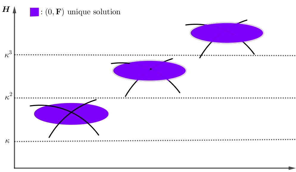
In the next theorem, we prove that (0,𝐅)\displaystyle(0,\mathbf{F}) is the unique minimizer of the functional when H/κ3\displaystyle H/\kappa^{3} is sufficiently large.

Theorem 3.2.

Let Ω⊂ℝ2\displaystyle\Omega\subset\mathbb{R}^{2} be a smooth, bounded, simply-connected open set. There exist positive constants C¯\displaystyle\bar{C} and κ0\displaystyle\kappa_{0}, such that, if

H≥C¯​κ3,κ≥κ0,H\geq\bar{C}\kappa^{3}\,,\qquad\kappa\geq\kappa_{0}\,,

then (0,𝐅)\displaystyle(0,\mathbf{F}) is the unique solution to (1.10).

Proof.

We denote by μ1N​(b​𝐅)\displaystyle\mu_{1}^{N}(b\mathbf{F}) the lowest eigenvalue of the Schr​o¨​dinger\displaystyle\rm Schr\ddot{o}dinger operator Pb​𝐅Ω\displaystyle P_{b\mathbf{F}}^{\Omega} with Neumann condition in L2​(Ω)\displaystyle L^{2}(\Omega). Assume that we have a non normal critical point (ψ,𝐀)\displaystyle(\psi,\mathbf{A}) for ℰκ,H,B0\displaystyle\mathcal{E}_{\kappa,H,B_{0}}. This means that (ψ,𝐀)∈H1​(Ω)×Hdiv1​(Ω)\displaystyle(\psi,\mathbf{A})\in H^{1}(\Omega)\times H^{1}_{{\rm div}}(\Omega) is a solution of (1.10) and

∫Ω|ψ|2​𝑑x>0.\int_{\Omega}|\psi|^{2}\,dx>0\,.

Using (3.1) with b=κ​H\displaystyle b=\kappa H, we get

‖(∇−i​b​𝐅)​ψ‖L2​(Ω)2‖ψ‖L2​(Ω)2≤κ2,\frac{\|(\nabla-ib\mathbf{F})\psi\|_{L^{2}(\Omega)}^{2}}{\|\psi\|^{2}_{L^{2}(\Omega)}}\leq\kappa^{2}\,,

which implies by assumption that the lowest Neumann eigenvalue satisfies,

μ1N​(b​𝐅)≤κ2.\mu_{1}^{N}(b\mathbf{F})\leq\kappa^{2}\,.

Using the leading order asymptotics in (2.1) with b=κ​H\displaystyle b=\kappa H and H≥C¯​κ3\displaystyle H\geq\bar{C}\kappa^{3}, we obtain

(3.4) Λ1=limκ​H⟶+∞μ1N​(κ​H​𝐅)κ​H≤C¯−12.\Lambda_{1}=\lim_{\kappa H\longrightarrow+\infty}\frac{\mu_{1}^{N}(\kappa H\mathbf{F})}{\sqrt{\kappa H}}\leq\bar{C}^{-\frac{1}{2}}\,.

For C¯>(Λ1)−2\displaystyle\bar{C}>(\Lambda_{1})^{-2}, (3.4) yields a contradiction. ∎

Refer to caption
Figure 4. Schematic representation of the levels of H\displaystyle H that correspond to the trivial solution (0,𝐅)\displaystyle(0,\mathbf{F}).

4. Criterion for the breakdown of superconductivity

The purpose of this section is to prove Theorem 1.3. One ingredient in the proof is Proposition 4.1 below on the localization of the order parameter, which is an adaptation of an analogous result obtained in [18] for the case where the magnetic field has a non-empty zero set but not self-intersecting. It says that, if (ψ,𝐀)\displaystyle(\psi,\mathbf{A}) is a critical point of the functional in (1.8) and H\displaystyle H is of order κ3\displaystyle\kappa^{3}, then |ψ|\displaystyle|\psi| is concentrated near the set Σ={x∈Ω:B0(x)=0,&∇B0(x)=0}\displaystyle\Sigma=\{x\in\Omega\penalty\ :\penalty\ B_{0}(x)=0,\&\,\nabla B_{0}(x)=0\}.

Proposition 4.1.

Let ε>0\displaystyle\varepsilon>0 and α∈(0,1)\displaystyle\alpha\in\left(0,1\right). There exist two positive constants C\displaystyle C and κ0\displaystyle\kappa_{0} such that, if

(4.1) κ≥κ0,H≥ε​κ3,\kappa\geq\kappa_{0}\,,\quad H\geq\varepsilon\,\kappa^{3}\,,

and (ψ,𝐀)\displaystyle(\psi,\mathbf{A}) is a solution of (1.10), then

(4.2) ‖ψ‖L2​(Ω)2≤C​κ−α2​‖ψ‖L4​(Ω)2.\|\psi\|^{2}_{L^{2}(\Omega)}\leq C\,\kappa^{-\frac{\alpha}{2}}\|\psi\|^{2}_{L^{4}(\Omega)}\,.
Proof.

Let ℓ=κ−α\displaystyle\ell=\kappa^{-\alpha} with 0<α<1\displaystyle 0<\alpha<1 and

Dℓ={x∈Ω:dist⁡(x,∂Ω)>ℓ&dist⁡(x,Γ)>ℓ}.D_{\ell}=\big\{x\in\Omega:\dist(x,\partial\Omega)>\ell\penalty\ \&\penalty\ \dist(x,\Gamma)>\ell\big\}\,.

Let us introduce a cut off function h∈Cc∞​(Ω)\displaystyle h\in C^{\infty}_{c}(\Omega) satisfying

0≤h≤1inΩ,h=1inDℓ,supph⊂Dℓ/2and|∇h|≤CℓinΩ,0\leq h\leq 1\penalty\ {\rm in}\penalty\ \Omega\,,\quad h=1\penalty\ {\rm in}\penalty\ D_{\ell}\,,\quad{\rm supp}\,h\subset D_{\ell/2}\quad{\rm and}\quad|\nabla h|\leq\frac{C}{\ell}\quad{\rm in}\penalty\ \Omega\,,

where C\displaystyle C is a positive constant.
Adapting the proof by Helffer and Kachmar [18, Equation (6.6)], there exists a positive constant c\displaystyle c such that,

κ​H​∫Ω|B0​(x)|​|h​ψ|2​𝑑x−c​κ​‖ψ‖L2​(Ω)​‖h​ψ‖L4​(Ω)2≤∫Ω|(∇−i​κ​H​𝐀)​h​ψ|2​𝑑x.\kappa\,H\int_{\Omega}|B_{0}(x)|\,|h\psi|^{2}\,dx-c\,\kappa\,\|\psi\|_{L^{2}(\Omega)}\|h\psi\|_{L^{4}(\Omega)}^{2}\leq\int_{\Omega}|(\nabla-i\kappa H\mathbf{A})h\psi|^{2}\,dx\,.

Using Cauchy’s inequality, we obtain

c​κ​‖ψ‖L2​(Ω)​‖h​ψ‖L4​(Ω)2≤c2​‖ψ‖L2​(Ω)2+κ2​‖h​ψ‖L4​(Ω)4,c\,\kappa\,\|\psi\|_{L^{2}(\Omega)}\|h\psi\|_{L^{4}(\Omega)}^{2}\leq c^{2}\|\psi\|_{L^{2}(\Omega)}^{2}+\kappa^{2}\|h\psi\|_{L^{4}(\Omega)}^{4}\,,

which implies that

(4.3) ∫Ω(κ​H​|B0​(x)|−κ2)​|h​ψ|2​𝑑x≤∫Ω|(∇−i​κ​H​𝐀)​h​ψ|2​𝑑x−κ2​‖h​ψ‖L2​(Ω)2+c2​‖ψ‖L2​(Ω)2+κ2​‖h​ψ‖L4​(Ω)4.\int_{\Omega}\,\left(\kappa\,H\,|B_{0}(x)|-\kappa^{2}\right)\,|h\psi|^{2}\,dx\leq\int_{\Omega}|(\nabla-i\kappa H\mathbf{A})h\psi|^{2}\,dx-\kappa^{2}\|h\psi\|_{L^{2}(\Omega)}^{2}\\ +c^{2}\|\psi\|_{L^{2}(\Omega)}^{2}+\kappa^{2}\|h\psi\|_{L^{4}(\Omega)}^{4}\,.

Multiplying both sides of (1.10)a by h2​ψ\displaystyle h^{2}\psi, it results from an integration by parts that,

(4.4) ∫Ω(|(∇−i​κ​H​𝐀)​h​ψ|2−κ2​|h​ψ|2)​𝑑x=∫Ω|∇h|2​|ψ|2​𝑑x−κ2​∫Ωh2​|ψ|4​𝑑x.\int_{\Omega}\Big(|(\nabla-i\kappa H\mathbf{A})h\psi|^{2}-\kappa^{2}|h\psi|^{2}\Big)\,dx=\int_{\Omega}|\nabla h|^{2}|\psi|^{2}\,dx-\kappa^{2}\int_{\Omega}h^{2}|\psi|^{4}\,dx\,.

Implementing (4.4) into (4.3), we get,

∫Ω(κ​H​|B0​(x)|−κ2)​|h​ψ|2​𝑑x\displaystyle\displaystyle\int_{\Omega}\,\left(\kappa\,H\,|B_{0}(x)|-\kappa^{2}\right)\,|h\psi|^{2}\,dx ≤c2​∫Ω|ψ|2​𝑑x+∫Ω|∇h|2​|ψ|2​𝑑x+κ2​∫Ω(h4−h2)​|ψ|4​𝑑x\displaystyle\displaystyle\leq c^{2}\int_{\Omega}|\psi|^{2}\,dx+\int_{\Omega}|\nabla h|^{2}|\psi|^{2}\,dx+\kappa^{2}\int_{\Omega}(h^{4}-h^{2})|\psi|^{4}\,dx
≤c2​∫Ω|ψ|2​𝑑x+∫Ω|∇h|2​|ψ|2​𝑑x.\displaystyle\displaystyle\leq c^{2}\int_{\Omega}|\psi|^{2}\,dx+\int_{\Omega}|\nabla h|^{2}|\psi|^{2}\,dx\,.

Here, we have used the fact that h4≤h2\displaystyle h^{4}\leq h^{2} since 0≤h≤1\displaystyle 0\leq h\leq 1.
As a consequence of the non degeneracy of B0\displaystyle B_{0} outside Γ\displaystyle\Gamma, there exists a positive constant C⁡(B0)\displaystyle C(B_{0}) such that

(4.5) |B0​(x)|≥C⁡(B0)​min⁡(dist​(x,Σ)2,dist⁡(x,Γ))≥C⁡(B0)​ℓ2,∀x∈Dℓ.|B_{0}(x)|\geq C(B_{0})\min\Big({\rm dist}(x,\Sigma)^{2},{\rm dist}(x,\Gamma)\Big)\geq C(B_{0})\,\ell^{2}\,,\qquad\forall x\in D_{\ell}\,.

Therefore, by using (4.1), we get,

(C⁡(B0)​ε​κ4−2​α−κ2)​∫Ω|h​ψ|2​𝑑x≤c2​∫Ω|ψ|2​𝑑x+∫Ω|∇h|2​|ψ|2​𝑑x.\Big(C(B_{0})\,\varepsilon\,\kappa^{4-2\alpha}-\kappa^{2}\Big)\int_{\Omega}|h\psi|^{2}\,dx\leq c^{2}\int_{\Omega}|\psi|^{2}\,dx+\int_{\Omega}|\nabla h|^{2}|\psi|^{2}\,dx\,.

Writing

(4.6) ∫Ω|ψ|2​𝑑x=∫Ω|h​ψ|2​𝑑x+∫Ω(1−h2)​|ψ|2​𝑑x\displaystyle\int_{\Omega}|\psi|^{2}\,dx=\int_{\Omega}|h\psi|^{2}\,dx+\int_{\Omega}(1-h^{2})|\psi|^{2}\,dx

and using the assumption on h\displaystyle h, we have,

(C⁡(B0)​ε​κ4−2​α−κ2−c2)​∫Ω|h​ψ|2​𝑑x≤(c2+C​κ2​α)​∫Ω∖Dℓ|ψ|2​𝑑x.\Big(C(B_{0})\,\varepsilon\,\kappa^{4-2\alpha}-\kappa^{2}-c^{2}\Big)\int_{\Omega}|h\psi|^{2}\,dx\leq\Big(c^{2}+C\,\kappa^{2\alpha}\Big)\int_{\Omega\setminus D_{\ell}}|\psi|^{2}\,dx\,.

For κ\displaystyle\kappa large enough, C⁡(B0)​ε​κ4−2​α−κ2−c2≥12​C​(B0)​ε​κ4−2​α\displaystyle\displaystyle C(B_{0})\,\varepsilon\,\kappa^{4-2\alpha}-\kappa^{2}-c^{2}\geq\frac{1}{2}C(B_{0})\,\varepsilon\,\kappa^{4-2\alpha} and

∫Ω|h​ψ|2​𝑑x≤2​CC⁡(B0)​ε​κ4​(α−1)​∫Ω∖Dℓ|ψ|2​𝑑x.\int_{\Omega}|h\psi|^{2}\,dx\leq 2\frac{C}{C(B_{0})\,\varepsilon}\,\kappa^{4(\alpha-1)}\int_{\Omega\setminus D_{\ell}}|\psi|^{2}\,dx\,.

Using the decomposition in (4.6) and that 1−h2\displaystyle 1-h^{2} vanishes outside Dℓ\displaystyle D_{\ell}, we get further,

∫Ω|ψ⁡(x)|2​𝑑x≤(2​CC⁡(B0)​ε​κ4​(α−1)+1)​∫Ω∖Dℓ|ψ|2​𝑑x≤2​∫Ω∖Dℓ|ψ|2​𝑑x.\int_{\Omega}|\psi(x)|^{2}\,dx\leq\left(2\frac{C}{C(B_{0})\,\varepsilon}\,\kappa^{4(\alpha-1)}+1\right)\int_{\Omega\setminus D_{\ell}}|\psi|^{2}\,dx\leq 2\int_{\Omega\setminus D_{\ell}}|\psi|^{2}\,dx\,.

Finally, by the Cauchy-Schwarz inequality,

∫Ω∖Dℓ|ψ|2​𝑑x≤|Ω∖Dℓ|1/2​(∫Ω∖Dℓ|ψ|4​𝑑x)12≤C​κ−α2​(∫Ω|ψ|4​𝑑x)12.\int_{\Omega\setminus D_{\ell}}|\psi|^{2}\,dx\leq|\Omega\setminus D_{\ell}|^{1/2}\left(\int_{\Omega\setminus D_{\ell}}|\psi|^{4}\,dx\right)^{\frac{1}{2}}\leq C\,\kappa^{-\frac{\alpha}{2}}\left(\int_{\Omega}|\psi|^{4}\,dx\right)^{\frac{1}{2}}\,.

This finishes the proof of the proposition. ∎

Proof of Theorem 1.3.

Suppose that (ψ,𝐀)\displaystyle(\psi,\mathbf{A}) is a solution of (1.10) with ‖ψ‖L2​(Ω)≠0\displaystyle\|\psi\|_{L^{2}(\Omega)}\neq 0. Then H≤C¯​κ3\displaystyle H\leq\bar{C}\kappa^{3}, where C¯>0\displaystyle\bar{C}>0 is the constant in Theorem 3.2.

We will prove that μ1​(κ​H​𝐅)<κ2\displaystyle\mu_{1}(\kappa H\mathbf{F})<\kappa^{2}. We distinguish between three cases:

  • Case 1:

    LetH≥ε​κ3\displaystyle H\geq\varepsilon\kappa^{3} and 0<ε<C¯\displaystyle 0<\varepsilon<\bar{C}. Multiplying (1.10)a by ψ\displaystyle\psi in L2​(Ω)\displaystyle L^{2}(\Omega) and using (1.10)c, we observe that,

    (4.7) κ2∥ψ∥L4​(Ω)4=−∫Ω(|(∇−iκH𝐀)ψ|2−κ2|ψ|2)dx.\kappa^{2}\|\psi\|_{L^{4}(\Omega)}^{4}=-\int_{\Omega}\Big(\big|(\nabla-i\kappa H\mathbf{A})\psi\big|^{2}-\kappa^{2}|\psi|^{2}\Big)\,dx\,.

    The Cauchy-Schwarz inequality yields for any δ∈(0,∞)\displaystyle\delta\in(0,\infty),

    (4.8) ∫Ω|(∇−i​κ​H​𝐀)​ψ|2​𝑑x≥(1−δ)​∫Ω|(∇−i​κ​H​𝐅)​ψ|2​𝑑x+(1−δ−1)​(κ​H)2​∫Ω|(𝐀−𝐅)​ψ|2​𝑑x.\int_{\Omega}|(\nabla-i\kappa H\mathbf{A})\psi|^{2}\,dx\geq(1-\delta)\int_{\Omega}|(\nabla-i\kappa H\mathbf{F})\psi|^{2}\,dx+(1-\delta^{-1})\,(\kappa H)^{2}\int_{\Omega}|(\mathbf{A}-\mathbf{F})\psi|^{2}\,dx\,.

    This implies that (after using the min-max principle),

    κ2​‖ψ‖L4​(Ω)4≤−(μ1​(κ​H​𝐅)+κ2)​‖ψ‖L2​(Ω)2+δ​‖(∇−i​κ​H​𝐅)​ψ‖L2​(Ω)2+δ−1​(κ​H)2​‖(𝐀−𝐅)​ψ‖L2​(Ω)2.\kappa^{2}\|\psi\|_{L^{4}(\Omega)}^{4}\leq-\Big(\mu_{1}(\kappa H\mathbf{F})+\kappa^{2}\Big)\,\|\psi\|_{L^{2}(\Omega)}^{2}+\delta\,\|(\nabla-i\kappa H\mathbf{F})\psi\|^{2}_{L^{2}(\Omega)}+\delta^{-1}(\kappa H)^{2}\|(\mathbf{A}-\mathbf{F})\psi\|_{L^{2}(\Omega)}^{2}\,.

    Using (3.2) and (3.3), we obtain,

    κ2​‖ψ‖L4​(Ω)4≤−(μ1​(κ​H​𝐅)+κ2)​‖ψ‖L2​(Ω)2+C​δ​κ2​‖ψ‖L2​(Ω)2+C′​δ−1​κ2​‖ψ‖L2​(Ω)2​‖ψ‖L4​(Ω)4.\kappa^{2}\|\psi\|_{L^{4}(\Omega)}^{4}\leq-\Big(\mu_{1}(\kappa H\mathbf{F})+\kappa^{2}\Big)\,\|\psi\|_{L^{2}(\Omega)}^{2}+C\,\delta\,\kappa^{2}\,\|\psi\|_{L^{2}(\Omega)}^{2}+C^{\prime}\,\delta^{-1}\,\kappa^{2}\,\|\psi\|_{L^{2}(\Omega)}^{2}\|\psi\|_{L^{4}(\Omega)}^{4}\,.

    From (4.2), we find that,

    κ2​‖ψ‖L4​(Ω)4≤−(μ1​(κ​H​𝐅)+κ2)​‖ψ‖L2​(Ω)2+C​δ​κ2−α2​‖ψ‖L4​(Ω)2+C′​δ−1​κ2−α2​‖ψ‖L4​(Ω)6.\kappa^{2}\|\psi\|_{L^{4}(\Omega)}^{4}\leq-\Big(\mu_{1}(\kappa H\mathbf{F})+\kappa^{2}\Big)\,\|\psi\|_{L^{2}(\Omega)}^{2}+C\,\delta\,\kappa^{2-\frac{\alpha}{2}}\,\|\psi\|_{L^{4}(\Omega)}^{2}+C^{\prime}\,\delta^{-1}\,\kappa^{2-\frac{\alpha}{2}}\,\|\psi\|_{L^{4}(\Omega)}^{6}\,.

    Remembering that ‖ψ‖L2​(Ω)≠0\displaystyle\|\psi\|_{L^{2}(\Omega)}\neq 0 and choosing δ=‖ψ‖L4​(Ω)2\displaystyle\delta=\|\psi\|_{L^{4}(\Omega)}^{2}, we get,

    (μ1​(κ​H​𝐅)+κ2)​‖ψ‖L2​(Ω)2≤κ2​‖ψ‖L4​(Ω)4​(C​κ−α2−1).\Big(\mu_{1}(\kappa H\mathbf{F})+\kappa^{2}\Big)\,\|\psi\|_{L^{2}(\Omega)}^{2}\leq\kappa^{2}\|\psi\|_{L^{4}(\Omega)}^{4}\left(C\,\kappa^{-\frac{\alpha}{2}}-1\right)\,.

    We deduce for κ\displaystyle\kappa sufficiently large μ1​(κ​H​𝐅)<κ2\displaystyle\mu_{1}(\kappa H\mathbf{F})<\kappa^{2}, which what we needed to prove the first case.

  • Case 2:

    Let c0​κ−1≤H<ε​κ3\displaystyle c_{0}\kappa^{-1}\leq H<\varepsilon\kappa^{3}, where c0>1\displaystyle c_{0}>1 is sufficiently large so that we can use Theorem 2.1 with b=κ​H\displaystyle b=\kappa H and M=0\displaystyle M=0. We observe as κ→+∞\displaystyle\kappa\to+\infty,

    μ1​(κ​H​𝐅)\displaystyle\displaystyle\mu_{1}(\kappa H\mathbf{F}) ≤(κ​H)12​|λ2Hess​(x)|1/2​𝒳1​(ε⁡(x))+C​(κ​H)14\displaystyle\displaystyle\leq(\kappa H)^{\frac{1}{2}}|\lambda^{\rm Hess}_{2}(x)|^{1/2}\mathcal{X}_{1}\Big(\varepsilon(x)\Big)+C\,(\kappa H)^{\frac{1}{4}}
    <κ2​ϵ12​|λ2Hess​(x)|1/2​𝒳1​(ε⁡(x))+C​κ.\displaystyle\displaystyle<\kappa^{2}\epsilon^{\frac{1}{2}}|\lambda^{\rm Hess}_{2}(x)|^{1/2}\mathcal{X}_{1}\Big(\varepsilon(x)\Big)+C\,\kappa\,.

    We can choose ε>0\displaystyle\varepsilon>0 such that ϵ12​|λ2Hess​(x)|1/2​𝒳1​(ε⁡(x))−1<0\displaystyle\epsilon^{\frac{1}{2}}|\lambda^{\rm Hess}_{2}(x)|^{1/2}\mathcal{X}_{1}\Big(\varepsilon(x)\Big)-1<0 to get,

    μ1​(κ​H​𝐅)<κ2,as​κ⟶+∞.\mu_{1}(\kappa H\mathbf{F})<\kappa^{2}\,,\qquad{\rm as}\penalty\ \kappa\longrightarrow+\infty\,.
  • Case 3:

    H<c0​κ−1\displaystyle H<c_{0}\kappa^{-1}. Let x0∈Ω\displaystyle x_{0}\in\Omega and let χℓ∈Cc∞​(Ω)\displaystyle\chi_{\ell}\in C_{c}^{\infty}(\Omega) be a cut-off function satisfying:

    (4.9) 0≤χℓ≤1inΩ,suppχℓ⊂B(x0,ℓ),χℓ=1inB(x0,ℓ2)and|∇χℓ|≤Cℓ.0\leq\chi_{\ell}\leq 1\penalty\ {\rm in}\penalty\ \Omega\,,\quad{\rm supp}\,\chi_{\ell}\subset B(x_{0},\ell)\,,\quad\chi_{\ell}=1\penalty\ {\rm in}\penalty\ B\left(x_{0},\frac{\ell}{2}\right)\quad{\rm and}\quad|\nabla\chi_{\ell}|\leq\frac{C}{\ell}\,.

    We may write,

    μ1​(κ​H​𝐅)≤∫Ω|(∇−i​κ​H​𝐅)​χℓ|2​𝑑x‖χℓ‖L2​(Ω)2.\mu_{1}(\kappa H\mathbf{F})\leq\frac{\displaystyle\int_{\Omega}|(\nabla-i\kappa H\mathbf{F})\chi_{\ell}|^{2}\,dx}{\|\chi_{\ell}\|_{L^{2}(\Omega)}^{2}}\,.

    Using the assumptions on χℓ\displaystyle\chi_{\ell} and the fact that 𝐅∈C∞​(Ω¯)\displaystyle\mathbf{F}\in C^{\infty}(\overline{\Omega}), a trivial estimate is,

    ∫Ω|(∇−i​κ​H​𝐅)​χℓ|2​𝑑x\displaystyle\displaystyle\int_{\Omega}|(\nabla-i\kappa H\mathbf{F})\chi_{\ell}|^{2}\,dx ≤∫B⁡(x0,ℓ)|∇χℓ|2​𝑑x+κ2​H2​∫B⁡(x0,ℓ)|𝐅​χℓ|2​𝑑x\displaystyle\displaystyle\leq\int_{B(x_{0},\ell)}|\nabla\chi_{\ell}|^{2}\,dx+\kappa^{2}H^{2}\int_{B(x_{0},\ell)}|\mathbf{F}\chi_{\ell}|^{2}\,dx
    (4.10) ≤C⁡(1+(κ​H​ℓ)2).\displaystyle\displaystyle\leq C\,(1+(\kappa\,H\,\ell)^{2})\,.

    This implies that

    (μ1​(κ​H​𝐅)−κ2)​‖χℓ‖L2​(Ω)2≤C⁡(1+(κ​H​ℓ)2)−(κ​ℓ)2.\Big(\mu_{1}(\kappa H\mathbf{F})-\kappa^{2}\Big)\|\chi_{\ell}\|_{L^{2}(\Omega)}^{2}\leq C\Big(1+(\kappa\,H\,\ell)^{2}\Big)-\,(\kappa\ell)^{2}\,.

    We select ℓ=κ−12\displaystyle\ell=\kappa^{-\frac{1}{2}} and remember that H<c0​κ−1\displaystyle H<c_{0}\,\kappa^{-1}. We find that,

    (μ1​(κ​H​𝐅)−κ2)​‖χℓ‖L2​(Ω)2<C⁡(1+κ−1)−κ,\Big(\mu_{1}(\kappa H\mathbf{F})-\kappa^{2}\Big)\|\chi_{\ell}\|_{L^{2}(\Omega)}^{2}<C\,(1+\kappa^{-1})-\kappa\,,

    and consequently, for κ\displaystyle\kappa sufficiently large,

    μ1​(κ​H​𝐅)<κ2.\mu_{1}(\kappa H\mathbf{F})<\kappa^{2}\,.

∎

References

  • [1] K. Attar. The ground state energy of the two-dimensional Ginzburg-Landau functional with variable magnetic field, Ann. I. H. Poincaré, vol. 32, 325-345 (2015).
  • [2] K. Attar. Pinning with a variable magnetic field of the two dimensional Ginzburg-Landau model, Nonlinear Analysis, vol. 139, 1-54 (2016).
  • [3] W. Assaad, A. Kachmar, M.P. Sundqvist. The Distribution of Superconductivity Near a Magnetic Barrier, Commun. Math. Phys. Vol. 366 (1), 269-332 (2019).
  • [4] W. Assaad. The breakdown of superconductivity in the presence of magnetic steps, Com. Cont. Mat.. Vol. 23(2), 2050005 (2021).
  • [5] V. Bonnaillie-Noël, S. Fournais. Superconductivity in domains with corners, Reviews in Mathematical Physics, Vol. 19(6), 607-637 (2007).
  • [6] V. Bonnaillie-Noël, N. Raymond. Breaking a magnetic zero locus: model operators and numerical approach, ZAMM Z. Angew. Math. Mech. Vol. 95, 120-139 (2015).
  • [7] M. Correggi, N. Rougerie. On the Ginzburg-Landau Functional in the Surface Superconductivity Regime, Commun. Math. Phys. vol. 332, 1297-1343 (2014).
  • [8] M. Dauge, J.P. Miqueu, N. Raymond. On the semiclassical Laplacian with magnetic field having self-intersecting zero set, J. Spectr. Theory. Vol 10(4), 1211-1252 (2020).
  • [9] N. Dombrowski, N. Raymond. Semiclassical analysis with vanishing magnetic fields, J. Spectr. Theory. vol 3, 423-464 (2013).
  • [10] S. Fournais, B. Helffer. On the third critical field in Ginzburg-Landau theory, Comm. Math. Phys. Vol. 226 (1), 153-196, (2006).
  • [11] S. Fournais, B. Helffer. Strong diamagnetism for general domains and application, Ann. Inst. Fourier. Vol 57(7), 2389-2400 (2007).
  • [12] S. Fournais, B. Helffer. On the Ginzburg-Landau critical field in three dimensions, Commun. Pure Appl. Math. vol 62(2), 215-241 (2009).
  • [13] S. Fournais, B. Helffer. Spectral Methods in Surface Superconductivity, Progress Nonlinear Differential Equations Appl., vol. 77, Birkha¨\displaystyle\ddot{a}user, Boston, (2010).
  • [14] S. Fournais, A. Kachmar. On the transition to the normal phase for superconductors surrounded by normal conductors, Journal of Differential Equations, vol. 247, 1637-1672 (2009).
  • [15] S. Fournais, A. Kachmar. Nucleation of bulk superconductivity close to critical magnetic field, Advances in Mathematics, vol. 226, 1213-1258 (2011).
  • [16] S. Fournais, M. Persson Sundqvist. Lack of Diamagnetism and the Little-Parks Effect, Commun. Math. Phy., 337, 191-224 (2015).
  • [17] T. Giorgi, D. Phillips. The breakdown of superconductivity due to strong fields for the Ginzburg-Landau model, Siam J. Math. Anal. vol. 30, 341-359 (1999).
  • [18] B. Helffer, A. Kachmar. The Ginzburg-Landau functional with vanishing magnetic field, Arch. Rational Mech. Anal., vol. 218, 55-122 (2015).
  • [19] B. Helffer, A. Kachmar. Thin domain limit and counterexamples to strong diamagnetism, Reviews in Mathematical Physics, vol. 33 (2), 2150003 (2021).
  • [20] A. Kachmar, X. B. Pan. Superconductivity and the Aharonov-Bohm effect, C. R. Acad. Sci. Paris, Ser. I. vol. 357, 216-220 (2019).
  • [21] A. Kachmar, X. B. Pan. Oscillatory patterns in the Ginzburg-Landau model driven by the Aharonov-Bohm potential, J. Funct. Anal. vol. 279 (10), 108718 (2020).
  • [22] A. Kachmar, M. P. Sundqvist. Counterexample to strong diamagnetism for the magnetic Robin Laplacian, Math. Phys. Anal. Geom. vol. 23 (27), 23-27 (2020).
  • [23] A. Kachmar, M. Wehbe. Averaging of magnetic fields and applications, arXiv:2003.04415 .
  • [24] T. Kato, Perturbation Theory for Linear Operators, Springer-Verlag, Berlin, (1976).
  • [25] K. Lu, X-B.Pan. Estimates of the upper critical field for the Ginzburg-Landau equations of superconductivity, Physica D., vol. 127, 73-104 (1999).
  • [26] W.A. Little, R.D. Parks. Observation of quantum periodicity in the transition temperature of a superconducting cylinder, Phys. Rev. Lett. vol.9(1), 9-12 (1962)
  • [27] R. Montgomery. Hearing the zero locus of a magnetic field, Comm. Math. Phys., vol. 168, 651-675 (1995).
  • [28] X.B. Pan, K.H. Kwek. Schrödinger operators with non-degenerately vanishing magnetic fields in bounded domains, Trans. Am. Math. Soc. vol. 354 (10), 4201-4227 (2002).
  • [29] X.B. Pan. Surface superconductivity in applied magnetic fields above HC2\displaystyle H_{C_{2}}, Comm. Math. Phys. vol. 228, 327-370 (2002).
  • [30] N. Raymond. Sharp Asymptotics for the Neumann Laplacian with Variable Magnetic Field: Case of Dimension 2, Ann. I. H. Poincaré. vol. 10, 95-122 (2009).
  • [31] E. Sandier, S.Serfaty. Ginzburg-Landau minimizers near the first critical field have bounded vorticity, Calc. Var. Partial Differential Equations. vol. 17 (1), 17-28 (2003).
  • [32] E. Sandier, S.Serfaty. The Decrease of Bulk-Superconductivity Close to the Second Critical Field in the Ginzburg-Landau Model, SIAM J. Math. Anal.. vol. 34 (4), 939-956 (2003).