Shear-induced phase transition and critical exponents in 3D fiber networks
Abstract
When subject to applied strain, fiber networks exhibit nonlinear elastic stiffening. Recent theory and experiements have shown that this phenomenon is controlled by an underlying mechanical phase transition that is critical in nature. Growing simulation evidence points to non-mean-field behavior for this transition and a hyperscaling relation has been proposed to relate the corresponding critical exponents. Here, we report simulations on two distinct network structures in 3D. By performing finite-size scaling analysis, we test hyperscaling and identify various critical exponents. From the apparent validity of hyperscaling, as well as the non-mean-field exponents we observe, our results suggest that the upper critical dimension for the strain-controlled phase transition is above three, in contrast to the jamming transition that represents another athermal, mechanical phase transition.
Networks of interconnected fibers are common in both natural and synthetic contexts, with examples ranging from biopolymer networks to paper and carbon nanotube materials Hough et al. 2004; Bryning et al. 2007; Dan et al. 2009. In biology, fibrous networks are primarily responsible for the mechanical stability of cells and tissues. These networks include both intracellular structures of actin and microtubules as well as extracellular matrices such as collagen and fibrin Fletcher and Mullins 2010; Pedersen and Swartz 2005. In recent decades, high precision rheology experiments on purified, reconstituted biopolymer networks have revealed unusual elastic properties including negative normal stresses Janmey et al. 2007 and nonlinear strain-stiffening Gardel et al. 2004; Storm et al. 2005. It has been shown that the mechanics of such networks depend not only on the elasticity of individual fibers but also strongly on network connectivity. To understand the mechanical behavior of stiff biopolymer networks, coarse-grained athermal fiber models with controlled connectivity have been used in literature Head et al. 2003a; Head et al. 2003b; Wilhelm and Frey 2003; Das et al. 2007; Wyart et al. 2008; Broedersz and MacKintosh 2014; Vermeulen et al. 2017. Strikingly, these simple models can accurately explain the strain stiffening observed in collagen experiments Sharma et al. 2016a; Jansen et al. 2018. Both experiments and theory point to the importance of a mechanical phase transition as a function of strain.
Here, we study the critical aspects of this phase transition in 3D fiber networks under applied simple shear. Most prior systematic studies have been limited to 2D, due to the significant computational challenges imposed by the nonlinear elasticity and the need for large systems because of the diverging correlation length. Although models to date point to qualitatively similar behavior in 2D and 3D Licup et al. 2015; Sharma et al. 2016a; Sharma et al. 2016b; Shivers et al. 2019a, important questions remain, e.g., concerning the possibility of non-mean-field behavior that has been observed in 2D. We show that fiber networks exhibit non-mean-field behavior in 3D and are consistent with a recently identified hyperscaling scaling relation Shivers et al. 2019b, suggesting that the upper critical dimension for fiber networks is greater than three, in contrast to the jamming transition Goodrich et al. 2014.

Model— We consider two varieties of network structures; packing-derived (PD) and random geometric graph (RGG) networks at physiologically-relevant connectivity Lindström et al. 2010; Lindström et al. 2013; Jansen et al. 2018. Importantly such connectivity lies below the 3D Maxwell isostatic threshold Maxwell 1870; Calladine 1978, at which central-force networks are marginally stable to linear order, as sketched in Fig. 1. This connectivity-controlled rigidity transition has been extensively studied in spring networks Feng and Sahimi 1985; Arbabi and Sahimi 1988; Wyart et al. 2008; Broedersz et al. 2011; Feng et al. 2016, and is analogous to jamming in granular materials Cates et al. 1998; Liu and Nagel 1998; van Hecke 2010, although the critical exponents differ.
For PD networks, we use a jammed packing of spheres to create an off-lattice network. We randomly distribute a 50-50 bidisperse mixture of spherical particles with size ratio of 1.4 in a periodic cube of size , with spheres in total. The particles interact via a repulsive harmonic potential O’Hern et al. 2002; O’Hern et al. 2003; Goodrich et al. 2014. We start by swelling the particles until the pressure becomes finite, which yields a network with . We then randomly remove bonds to obtain the desired connectivity . For RGG networks, we randomly distribute nodes in a cube with side length before connecting pairs of nodes according to a distance-dependent probability distribution Beroz et al. 2017 until the desired connectivity is reached.
The network elastic energy consists of stretching and bending contributions
| (1) |
where is the stretching modulus of the individual bonds, is the initial bond length prior to any deformation, is the current bond length, is the bending stiffness of fibers, is the initial angle between two adjacent bonds and prior to any deformation, is the current angle between adjacent bonds and , and is the initial average bond length of bonds and . We set and vary the dimensionless bending stiffness , where is average initial bond length.
To study the mechanical transition, we apply a simple shear deformation in a step-wise manner in the plane using Lees-Edwards boundary conditions Lees and Edwards 1972. Although we focus on shear, we note that uniaxial and bulk deformations can also rigidify such networks Sheinman et al. 2012; van Oosten et al. 2016; Vahabi et al. 2016; Arzash et al. 2019; Merkel et al. 2019. Using the FIRE algorithm Bitzek et al. 2006, we minimize the elastic energy defined in Eq. (1) at each strain step and calculate the stress tensor as Shivers et al. 2019b
| (2) |
where is the volume of system, is the component of the force exerted on node by node , and is the component of the displacement vector connecting nodes and . We then compute the differential shear modulus as . Unless otherwise stated, quantities reported throughout the paper correspond to averages over 40 random realizations.
Scaling relation— When we apply sufficiently large shear strain to a subisostatic network with central-force interactions (red arrow in Fig. 1), the system undergoes a phase transition from a floppy to a rigid state. At the critical strain , which is a function of network connectivity Wyart et al. 2008; Sharma et al. 2016a, the differential shear modulus discontinuously jumps from 0 to a finite value Vermeulen et al. 2017; Merkel et al. 2019; Arzash et al. 2020. The excess shear modulus exhibits a power law scaling behavior near , with , where . Including weak bending interactions between adjacent bonds stabilizes the network in the subcritical regime , such that the floppy-to-rigid transition becomes a transition between bending- and stretching-dominated states. The following Widom-like Widom 1965 scaling function captures the mechanics of networks with finite bending stiffness Sharma et al. 2016a
| (3) |
in which the positive and negative branches of the scaling function correspond to and , respectively. For and , the shear modulus scales as with . We note that continuity of as a function of requires that when is large.
To relate the scaling exponents near the critical strain , we follow the approach of Kadanoff Kadanoff 1966 for the elastic energy per node as a function of the small parameters and Shivers et al. 2019b. Rescaling the system by a factor results in a renormalized energy , in which and are the renormalized variables after transformation and is dimensionality. We assume that and near the critical point, with positive and . We can therefore write the elastic energy per node as Shivers et al. 2019b
| (4) |
We find the differential shear modulus from the second derivative with respect to or , in a way analogous to the heat capacity in a thermal phase transition, in which case differentiation is with respect to the temperature. Here, represents the second partial derivative of with respect to the first argument. So far, the rescaling factor is simply mathematical parameter that has not been specified. Thus, physical quantities such as cannot depend on , from which the form of Eq. (3) follows Kadanoff et al. 1967. By choosing , we find that for . We also identify the correlation length and the scaling relations Shivers et al. 2019b; Kadanoff et al. 1967
| (5) |
The first of these is a hyperscaling relation that is of particular importance for the appearance of the dimensionality of the system. This can can only be satisfied for mean-field systems at a particular , which sets the upper critical dimension. Only for dimensionality below this are non-mean-field critical exponents possible.
Results— In order to find the critical exponent , care must be taken to account for finite size effects. For a finite system, only when the system size exceeds the the correlation length , i.e., , will the thermodynamic properties approximate those of the thermodynamic limit. In the opposite limit , which occurs close to , correlations are limited and analytic behavior is expected. Thus, we determine the critical exponents only for . For small , we expect the shear modulus to vary with system size as Arzash et al. 2020
| (6) |
Here, is a scaling function that is expected to increase as for large arguments, in order to obtain a well-defined thermodynamic limit. Figure 2 shows the finite-size analysis corresponding to this. Here, the sample-dependent critical strain is found using the bisection method Merkel et al. 2019; Arzash et al. 2020. For PD networks at of size at strains beyond the regime dominated by finite-size effects (i.e., ) we find , where the errors are standard deviations for 20 random realizations. Upon increasing the connectivity to , the resulting data are consistent with a slightly larger , which is obtained by averaging 20 samples of size (see Fig. 2). The distributions of the exponent are shown as insets in Fig. 2. For the RGG model at we find using a system size of . 11 1 We note that the RGG model, similar to lattice-based models, has long straight fibers. In this case, for small system sizes, small connected clusters of nearly aligned bonds can span the length of the simulation box. These clusters, which may comprise only a small fraction of the network’s bonds, nonetheless determine the critical strain at which the becomes nonzero. As a result, in some cases, such networks exhibit an apparent two-branch behavior, with a regime of unusually low stiffness immediately above the critical strain followed by a more typical stiffening regime at larger strains. Similar behavior has been observed in 2D triangular networks Arzash et al. 2020. We demonstrate this effect for a set of RGG network samples in Fig. A.3 in the Appendix. To calculate for RGG networks, we removed samples exhibiting this two-branch behavior from our ensemble (see the discussion in the Appendix).
Similar to 2D models Arzash et al. 2020, we find that the shear modulus discontinuity decreases as system size increases (see Fig. A.1 in the Appendix). We note that as network size increases, the regime over which can be computed extends to smaller . Here, a non-mean-field exponent of is seen. In the finite size-dominated regime, however, the data are consistent with , which can be explained by a leading first term in the scaling function that becomes analytic when , as previously seen in 2D fiber networks Arzash et al. 2020 and jammed systems Goodrich et al. 2012.

In Fig. 3a, we plot the shear modulus versus strain for packing-derived networks with finite and . From the value of above, we find the critical exponent in the subcritical regime from Eq. (3). Since must be proportional to in this regime, we expect (see inset). The distribution of values with is shown in the inset of Fig. 3b. Considering Eq. (3), we expect to find a scaling collapse of data in Fig. 3a for various values to a single master curve. Figure 3b shows this Widom-like scaling analysis. As we can see, using the obtained values of and the data collapse in two branches, one for the data above , one for the data below . Figures A.6 and A.7 in the Appendix show similar analysis for RGG model with finite bending rigidity that results in .
One of the most striking features of a critical phase transition is the divergence of fluctuations at the critical point, along with the divergent correlation length for these fluctuations. Here, we measure the nonaffine displacement fluctuations of network nodes under an infinitesimal shear strain, defined as
| (7) |
where the and are the relaxed and affine displacement vectors of network nodes, respectively, after applying a small strain , is the average initial bond length of the network, and the angular brackets represent an average over all nodes. For central-force networks, the fluctuations diverge as the network approaches the critical strain Sharma et al. 2016b. Since the nonaffine displacements are found by minimizing the energy , we expect that for small but finite . Therefore, the fluctuations diverge as Shivers et al. 2019b; Broedersz 2011
| (8) |
where the same is observed for both and .
To verify the scaling relation in Eq. (5), we calculate the nonaffine fluctuations for networks with , as shown for various system sizes in Fig. A.2 in the Appendix. From Eq. (8), we expect the following scaling form to capture the behavior of in finite simulations: Sharma et al. 2016b
| (9) |
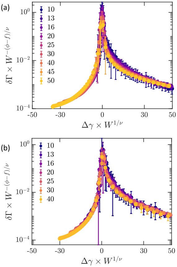
where is a scaling function and . Figure 4a shows the finite-size scaling collapse of data using the previously obtained values of and . The correlation length exponent is computed from the scaling relation in Eq. (5). Thus, this collapse demonstrates the validity of the hyperscaling relation in 3D systems. A similar scaling collapse of fluctuations is shown in Fig. 4b for the RGG model at . In order to further test this, we also simulated 3D PD networks at a different connectivity . The figures for this are shown in Figs. A.9-13 in the Appendix. The scaling exponents and are slightly larger than the corresponding exponents for networks with . With these new scaling exponents, we perform a similar finite-size scaling analysis to Fig. 4 and find further evidence that the hyperscaling relation holds.
Conclusion— In this study, we measure the exponents associated with the strain-driven rigidity transition for subisostatic 3D spring networks under applied simple shear. In agreement with previous work on various network architectures Sharma et al. 2016a; Rens et al. 2016; Shivers et al. 2019b, we find non-mean-field exponents in the critical regime by performing a systematic finite-size analysis in our 3D computational models. We also demonstrate evidence to support a recently proposed hyperscaling relation between critical exponents Shivers et al. 2019b. Taken together, these results point to an upper critical dimension for the strain-controlled phase transition that is above three, in stark contrast to the jamming transition Goodrich et al. 2014. While our focus here has been on the subisostatic transition that is most relevant to fiber networks such as collagen, it is interesting to note that the isostatic critical point corresponding to in 3D has also been shown to exhibit non-mean-field exponents Broedersz et al. 2011. In future work, it will be interesting to study hyperscaling for that transition as well.
Acknowledgments
This work was supported in part by the National Science Foundation Division of Materials Research (Grant DMR-1826623) and the National Science Foundation Center for Theoretical Biological Physics (Grant PHY-2019745).
References
- Hough et al. (2004) L. A. Hough, M. F. Islam, P. A. Janmey, and A. G. Yodh, Physical Review Letters 93, 168102 (2004).
- Bryning et al. (2007) M. B. Bryning, D. E. Milkie, M. F. Islam, L. A. Hough, J. M. Kikkawa, and A. G. Yodh, Advanced Materials 19, 661 (2007).
- Dan et al. (2009) B. Dan, G. C. Irvin, and M. Pasquali, ACS Nano 3, 835 (2009).
- Fletcher and Mullins (2010) D. A. Fletcher and R. D. Mullins, Nature 463, 485 (2010).
- Pedersen and Swartz (2005) J. A. Pedersen and M. A. Swartz, Annals of Biomedical Engineering 33, 1469 (2005).
- Janmey et al. (2007) P. A. Janmey, M. E. McCormick, S. Rammensee, J. L. Leight, P. C. Georges, and F. C. MacKintosh, Nature Materials 6, 48 (2007), number: 1 Publisher: Nature Publishing Group.
- Gardel et al. (2004) M. L. Gardel, J. H. Shin, F. C. MacKintosh, L. Mahadevan, P. Matsudaira, and D. A. Weitz, Science 304, 1301 (2004).
- Storm et al. (2005) C. Storm, J. J. Pastore, F. C. MacKintosh, T. C. Lubensky, and P. A. Janmey, Nature 435, 191 (2005), number: 7039 Publisher: Nature Publishing Group.
- Head et al. (2003a) D. A. Head, A. J. Levine, and F. C. MacKintosh, Physical Review Letters 91, 108102 (2003a).
- Head et al. (2003b) D. A. Head, A. J. Levine, and F. C. MacKintosh, Physical Review E 68, 061907 (2003b).
- Wilhelm and Frey (2003) J. Wilhelm and E. Frey, Physical Review Letters 91, 108103 (2003).
- Das et al. (2007) M. Das, F. C. MacKintosh, and A. J. Levine, Physical Review Letters 99, 038101 (2007).
- Wyart et al. (2008) M. Wyart, H. Liang, A. Kabla, and L. Mahadevan, Physical Review Letters 101, 215501 (2008).
- Broedersz and MacKintosh (2014) C. P. Broedersz and F. C. MacKintosh, Reviews of Modern Physics 86, 995 (2014).
- Vermeulen et al. (2017) M. F. J. Vermeulen, A. Bose, C. Storm, and W. G. Ellenbroek, Physical Review E 96, 053003 (2017).
- Sharma et al. (2016a) A. Sharma, A. J. Licup, K. A. Jansen, R. Rens, M. Sheinman, G. H. Koenderink, and F. C. MacKintosh, Nature Physics 12, 584 (2016a).
- Jansen et al. (2018) K. A. Jansen, A. J. Licup, A. Sharma, R. Rens, F. C. MacKintosh, and G. H. Koenderink, Biophysical Journal 114, 2665 (2018).
- Licup et al. (2015) A. J. Licup, S. Münster, A. Sharma, M. Sheinman, L. M. Jawerth, B. Fabry, D. A. Weitz, and F. C. MacKintosh, Proceedings of the National Academy of Sciences of the United States of America 112, 9573 (2015).
- Sharma et al. (2016b) A. Sharma, A. J. Licup, R. Rens, M. Vahabi, K. A. Jansen, G. H. Koenderink, and F. C. MacKintosh, Physical Review E 94, 042407 (2016b).
- Shivers et al. (2019a) J. L. Shivers, J. Feng, A. Sharma, and F. C. MacKintosh, Soft Matter 15, 1666 (2019a).
- Shivers et al. (2019b) J. L. Shivers, S. Arzash, A. Sharma, and F. C. MacKintosh, Physical Review Letters 122, 188003 (2019b).
- Goodrich et al. (2014) C. P. Goodrich, S. Dagois-Bohy, B. P. Tighe, M. van Hecke, A. J. Liu, and S. R. Nagel, Physical Review E 90, 022138 (2014).
- Lindström et al. (2010) S. B. Lindström, D. A. Vader, A. Kulachenko, and D. A. Weitz, Physical Review E 82, 051905 (2010).
- Lindström et al. (2013) S. B. Lindström, A. Kulachenko, L. M. Jawerth, and D. A. Vader, Soft Matter 9, 7302 (2013).
- Maxwell (1870) J. C. Maxwell, Transactions of the Royal Society of Edinburgh 26, 1 (1870).
- Calladine (1978) C. R. Calladine, International Journal of Solids and Structures 14, 161 (1978).
- Feng and Sahimi (1985) S. Feng and M. Sahimi, Physical Review B 31, 1671 (1985).
- Arbabi and Sahimi (1988) S. Arbabi and M. Sahimi, Physical Review B 38, 7173 (1988).
- Broedersz et al. (2011) C. P. Broedersz, X. Mao, T. C. Lubensky, and F. C. MacKintosh, Nature Physics 7, 983 (2011).
- Feng et al. (2016) J. Feng, H. Levine, X. Mao, and L. M. Sander, Soft Matter 12, 1419 (2016).
- Cates et al. (1998) M. E. Cates, J. P. Wittmer, J.-P. Bouchaud, and P. Claudin, Physical Review Letters 81, 1841 (1998).
- Liu and Nagel (1998) A. J. Liu and S. R. Nagel, Nature 396, 21 (1998).
- van Hecke (2010) M. van Hecke, Journal of Physics: Condensed Matter 22, 033101 (2010).
- O’Hern et al. (2002) C. S. O’Hern, S. A. Langer, A. J. Liu, and S. R. Nagel, Physical Review Letters 88, 075507 (2002).
- O’Hern et al. (2003) C. S. O’Hern, L. E. Silbert, A. J. Liu, and S. R. Nagel, Physical Review E 68, 011306 (2003).
- Beroz et al. (2017) F. Beroz, L. M. Jawerth, S. Münster, D. A. Weitz, C. P. Broedersz, and N. S. Wingreen, Nature Communications 8, 16096 (2017), number: 1 Publisher: Nature Publishing Group.
- Lees and Edwards (1972) A. W. Lees and S. F. Edwards, Journal of Physics C: Solid State Physics 5, 1921 (1972).
- Sheinman et al. (2012) M. Sheinman, C. P. Broedersz, and F. C. MacKintosh, Physical Review E 85, 021801 (2012).
- van Oosten et al. (2016) A. S. G. van Oosten, M. Vahabi, A. J. Licup, A. Sharma, P. A. Galie, F. C. MacKintosh, and P. A. Janmey, Scientific Reports 6, 19270 (2016), number: 1 Publisher: Nature Publishing Group.
- Vahabi et al. (2016) M. Vahabi, A. Sharma, A. J. Licup, A. S. G. van Oosten, P. A. Galie, P. A. Janmey, and F. C. MacKintosh, Soft Matter 12, 5050 (2016).
- Arzash et al. (2019) S. Arzash, J. L. Shivers, A. J. Licup, A. Sharma, and F. C. MacKintosh, Physical Review E 99, 042412 (2019).
- Merkel et al. (2019) M. Merkel, K. Baumgarten, B. P. Tighe, and M. L. Manning, Proceedings of the National Academy of Sciences 116, 6560 (2019).
- Bitzek et al. (2006) E. Bitzek, P. Koskinen, F. Gähler, M. Moseler, and P. Gumbsch, Physical Review Letters 97, 170201 (2006).
- Arzash et al. (2020) S. Arzash, J. L. Shivers, and F. C. MacKintosh, Soft Matter 16, 6784 (2020), publisher: The Royal Society of Chemistry.
- Widom (1965) B. Widom, The Journal of Chemical Physics 43, 3898 (1965).
- Kadanoff (1966) L. P. Kadanoff, Physics Physique Fizika 2, 263 (1966).
- Kadanoff et al. (1967) L. P. Kadanoff, W. Götze, D. Hamblen, R. Hecht, E. A. S. Lewis, V. V. Palciauskas, M. Rayl, J. Swift, D. Aspnes, and J. Kane, Reviews of Modern Physics 39, 395 (1967).
- (48) We note that the RGG model, similar to lattice-based models, has long straight fibers. In this case, for small system sizes, small connected clusters of nearly aligned bonds can span the length of the simulation box. These clusters, which may comprise only a small fraction of the network’s bonds, nonetheless determine the critical strain at which the becomes nonzero. As a result, in some cases, such networks exhibit an apparent two-branch behavior, with a regime of unusually low stiffness immediately above the critical strain followed by a more typical stiffening regime at larger strains. Similar behavior has been observed in 2D triangular networks Arzash et al. 2020. We demonstrate this effect for a set of RGG network samples in Fig. A.3 in the Appendix. To calculate for RGG networks, we removed samples exhibiting this two-branch behavior from our ensemble (see the discussion in the Appendix).
- Goodrich et al. (2012) C. P. Goodrich, A. J. Liu, and S. R. Nagel, Physical Review Letters 109, 095704 (2012).
- Broedersz (2011) C. P. Broedersz, Mechanics and dynamics of biopolymer networks, PhD Thesis, Vrije Universiteit Amsterdam (2011).
- Rens et al. (2016) R. Rens, M. Vahabi, A. J. Licup, F. C. MacKintosh, and A. Sharma, The Journal of Physical Chemistry B 120, 5831 (2016).
Appendix
3D PD networks at
3D RGG networks at
When subjected to nonlinear strains, network structures with long straight fibers such as lattice-based and RGG models are more likely to show an interesting finite-size effect. At the critical strain, these networks can be rigidified by a small connected cluster of consecutive bonds. This small cluster is responsible for the network stability until the strain becomes large enough to involve a larger portion of network bonds. Therefore the participation ratio of bonds, defined as the ratio of bonds under finite force to all bonds, exhibit a jump between a small value to a larger one. This results in a two-branch behavior in the shear modulus , as can be observed in Fig. A.3. As the network size becomes larger, its geometric structure becomes more isotropic, hence this artifact occurs less frequently. However, since we are dealing with 3D systems, it is computationally challenging to simulate large system sizes. As a result, significant number of random samples of our RGG model exhibit this finite-size effect. Note that because of the isotropic nature of PD models, this artifact is rare in those networks.
Since the shear modulus for the samples with a two-branch behavior cannot be fit as a power-law, we remove these samples when calculating the exponent. Figure A.4 b shows the finite-size scaling analysis of for the RGG model at after removing these samples.
3D PD networks at
The following figures are showing the same analysis that has been performed in the main text for a different network connectivity . The scaling exponents are close to what we obtained for networks at . These data again confirm that the scaling relation works in 3D. For all of following figures, the data are obtained by averaging 40 random realizations.