Fault-tolerant resource estimate for quantum chemical simulations: Case study on Li-ion battery electrolyte molecules
Abstract
We estimate the resources required in the fusion-based quantum computing scheme to simulate electrolyte molecules in Li-ion batteries on a fault-tolerant, photonic quantum computer. We focus on the molecules that can provide practical solutions to industrially relevant problems. Certain fault-tolerant operations require the use of single-qubit “magic states” prepared by dedicated “magic state factories” (MSFs). Producing and consuming magic states in parallel is typically a prohibitively expensive task, resulting in the serial application of fault-tolerant gates. However, for the systems considered, the MSF constitutes a negligible fraction of the total footprint of the quantum computer, allowing for the use of multiple MSFs to produce magic states in parallel. We suggest architectural and algorithmic techniques that can accommodate such a capability. We propose a method to consume multiple magic states simultaneously, which can potentially lead to an order of magnitude reduction in the computational runtime without additional expense in the footprint.
I Introduction
Quantum computers are capable of carrying out computational tasks that are intractable for classical computers, such as integer factorization Shor 1994, combinatorial optimization Pagano et al. 2020, simulation of interacting quantum many-body systems Feynman 1982; Lloyd 1996, and quantum chemistry McArdle et al. 2020 to name a few.
One of the most anticipated applications of quantum computers is first-principles quantum chemical simulation of complex molecules Muller and Blume-Kohout 2015. While such studies can be performed on classical computers as well, the computational cost typically scales exponentially unless one adopts certain assumptions and approximations Jiang et al. 2012; Weymuth et al. 2014. Quantum computers are expected to enable quantum chemical simulation from first-principles — with fewer assumptions and approximations — and thus accurately model the properties of various molecules. In turn, such studies may lead to new insights into those molecules that are otherwise difficult to obtain.
Recently, there have been continued innovative developments in quantum algorithms for quantum chemistry Poulin et al. 2014; Reiher et al. 2017; Babbush et al. 2018; Berry et al. 2019; von Burg et al. 2020; Lee et al. 2020; Rice et al. 2021; Gujarati et al. 2021; Takeshita et al. 2020; Su et al. 2021, which have led to many orders of magnitude reduction in the resources required to simulate molecules at accuracies beyond the reach of classical computation. These developments have been driven by a focus on a few molecular systems that take part in complex reactions that underlie high-impact open problems in chemistry (e.g., elucidating the mechanism of nitrogen fixation at FeMoco active sites Reiher et al. 2017; Li et al. 2019). Importantly, the cost reduction techniques found in these studies are expected to be applicable to other chemical systems as well.
Thus, it is of interest to understand the cost of these state-of-the-art algorithms when applied to a broader class of industrially relevant quantum chemistry problems and their corresponding molecular systems. In this article, we propose one such concrete application: the study of electrolyte molecules for Li-ion batteries. In conventional Li-ion batteries, the liquid electrolyte plays an important role in determining the performance and the stability of the batteries. Quantum chemical simulation of the underlying constituent molecules can help us better understand electrochemical reactions occurring in the liquid electrolytes, and serve as a useful guide in establishing design principles for better electrolytes.
Realizing the promise of quantum computation to accurately simulate complex chemical systems like Li-ion battery electrolyte chemistries will require devices capable of executing hundreds of billions of operations on thousands of logical qubits. Currently, a huge technological effort is underway to build a fault-tolerant quantum computer. As attention in the field turns toward engineering noise-resilient devices capable of performing such large computations, it is increasingly important to move beyond hardware-agnostic resource estimates in terms of qubits and gates, and account for the overhead of fault-tolerance.
In that spirit, we first describe resource estimates in terms of architecture-agnostic parameters like the number of qubits and gates, followed by compilation of these hardware-agnostic parameters into the standard primitives of our fault-tolerant architecture, culminating in architecture-specific size and runtime estimates. The fully-compiled resource estimate is markedly different to prior studies, in that it makes use of the recently-introduced fusion-based quantum computation (FBQC) scheme Bartolucci et al. 2021; Bombin et al. 2021.
FBQC is a quantum computing paradigm in which the fundamental building blocks of the computation are resource states; joint, entangling measurements called fusions; and feed-forward operations. For a conceptual overview of FBQC, see Appendix A. A promising technology that can realize these operations in practice is photonics Bartolucci et al. 2021. Physically, the resource states can be created using a resource state generator (RSG), a gadget that emits the resource states encoded in a finite number of photons Bartolucci et al. 2021. The requisite fusion measurements can be performed in a variety of ways using only linear optical elements and photon-detection Browne and Rudolph 2005; Bartolucci et al. 2021.
A salient feature of the photon-based FBQC scheme is the possibility of interleaving Bombin et al. 2021. Photons can be stored in an optical delay line of large length without significantly degrading the quality of the photonic qubits. This leads to a compelling ability to easily trade off between the footprint of the device and the runtime of the computation, potentially leading to a more modest engineering overhead in building a large-scale quantum computer. Naturally, the overall cost of the algorithm will greatly depend on the length of the delay line.

Taking into account the distinctive features of FBQC, we perform a detailed analysis of the resources required to simulate a variety of molecules relevant to Li-ion electrolyte chemistry on a fault-tolerant quantum computer. The result of this analysis is succinctly summarized in Fig. 1.
The scope of this article is really two-fold: after first providing concrete, fully-compiled resource estimates on the cost of simulating the aforementioned chemical systems, we study the degree to which considerations of parallelization at both the algorithmic and architectural level can reduce the overall resource requirements to perform these algorithms. Certain fault-tolerant operations require the use of single-qubit “magic states” prepared by dedicated “magic state factories” (MSFs) Bravyi and Kitaev 2005. According to our resource estimates, having an MSF that produces magic states serially is suboptimal for simulating the systems under consideration. For small quantum algorithms (i.e., few qubits and gates), the footprint of the factory constitutes a substantial fraction of the quantum computer; see Ref. Gidney and Fowler 2019; Litinski 2019a; Litinski 2019b for recent attempts to optimize the factory. However, as the number of logical qubits needed for the algorithm increases, the relative size of the MSF will become smaller. In that regime, the (relative) extra cost of adding another magic state factory will be small; while it has been known that this will happen eventually as the number of logical qubits increases (for instance, recent studies Lee et al. 2020; Gidney and Ekera 2019 have considered multiple MSFs in their estimates), the exact point where this crossing occurs has remained unaddressed in the literature. We fill this gap by performing a detailed study; the answer, which depends on the number of qubits and the T-gate count, is plotted in Fig. 1. Our study suggests that there are quantum algorithms with practical applications that lie outside the oft-assumed regime in which the size of the MSF is relatively large.
For these “intermediate”-sized fault-tolerant quantum computations, it is beneficial to use multiple MSFs, and to use them efficiently. We provide algorithmic and architectural adjustments that can accommodate the injection of multiple distilled magic states whilst making the Clifford gate count relatively small. On the algorithmic front, we perform a detailed analysis on the cost of parallelizing some of the key subroutines in quantum chemistry simulation algorithms. While many of the results we summarize in this paper are well-known, some are new. For example, we introduce a novel method to apply a specific sequence of Givens rotations used in fermionic basis change (i.e., “Gizens” rotations) in logarithmic depth (a proof is provided in Appendix E). On the architectural side, our work builds upon the scheme of Litinski Litinski 2019a, which is an architecture that can implement an arbitrary quantum algorithm using T-gates in time, where is the code distance of the individual logical qubits, independent of the number of Clifford gates in the algorithm. We propose a further optimization of this architecture, leading to a computation time of for a variable parameter while maintaining the code distance without increasing the footprint, assuming that (i) is small compared to and (ii) that the circuit is structured in such a way that T-gates can be applied simultaneously in the same time step.
We emphasize that while the explicit resource estimates of RSG count and runtime only apply to the FBQC paradigm, the results in other sections (particularly on the size of the magic state factories) apply more generally to any surface code-based architecture. The parallelization techniques detailed in this article may reduce the runtime requirements by an order of magnitude; however, while the numerical results were based on a Monte Carlo simulation, the performance of our new architectural proposal that uses multiple MSFs has not been simulated in detail. We leave this to future studies.
II Materials and Methods
We first describe the Li-ion battery chemistry use-case and the molecules under consideration and detail the classical computational pipeline required to specify the problem and the quantities of interest, then we describe the quantum algorithms we use to calculate the quantities of interest and quantify the resources required to implement these algorithms using a fault-tolerant cost model. We then detail how we convert these hardware-agnostic estimates into architecture-specific size and runtime estimates.
II.1 Battery chemistry use-case
In conventional Li-ion batteries, the liquid electrolyte plays an important role in determining the performance and stability of the batteries Goodenough and Kim 2010; Xu 2004; Weber et al. 2019. Electrolytes consist of three components; solvent molecules like ethylene carbonate (EC), conducting-salt molecules like LiPF6, and additive molecules like fluoroethylene carbonate (FEC). The solvent is the host for the salt and the additive, and thus needs to have high solvation, low viscosity, inertness, and safety. Conducting-salts dissociate into ions in the solvent, and these ions carry electricity and thus need to have sufficient solubility into solvent and high stability against side reactions with other chemical components. Additives are substances added to electrolytes to enhance specifically targeted properties, and need to provide durable performance in the long term.
Quantum chemical simulation can be used to understand the electrochemical reactions that occur in these constituent molecules, and thus aid in designing better electrolytes Urban et al. 2016; Wang et al. 2018a; Zhang 2006. As an example, let us assume that we aim to elaborate the effect of additives to Li-ion solvation Im et al. 2017. Although the entire process involves several intermediate steps and may evolve along different reaction paths, the Li-ion solvation ultimately requires Li to dissociate from salt molecules. Quantum chemical simulation can be used to calculate the dissociation energy of the salt molecules in two different environments: one with solvent-only, and another with solvent as well as additives. In the classical chemical regime, we are interested in determining the reaction rate, a quantitative proxy for the relative dominance of two chemical reactions. This quantity is proportional to the Boltzmann factor of the change in enthalpy of the two reactions. Thus, the calculated Li-dissociation energies can be used to determine which environment is more favorable for both the Li-dissociation as well as the solvation, quantitatively.
While quantum chemical simulation can be carried out from first-principles (solving Schrödinger’s equation without approximations), it is common to adopt approximations and assumptions because of the high computational expense originating from the exponentially-scaling complexity in a first-principles approach. Although such approximations and assumptions have been practically applied to a variety of chemical studies at a compromised accuracy, there is a fundamental limit in both the accuracy of simulation results and the spectrum of chemical systems that can be simulated. In particular, as the focus of chemical studies continues to shift to smaller-scales and evolves to include more comprehensive descriptions of the environments the chemical systems under study inhabit, demand for more precise simulations consistently increases. Quantum computers are believed to mitigate the exponentially-scaling computational complexities in certain problems and thus enable quantum chemical simulations in a full configuration-interaction scheme.
In this study, we take EC, LiPF6, and FEC to represent the solvent, conducting-salt, and additive molecules, respectively. We estimate the computational resources required to study their interactions with Li ions via quantum chemical simulation. Our proposed scenario is to perform the geometric optimization using density functional theory (DFT) calculations classically, and then calculate the energy via quantum computation. We consider quantum phase estimation (QPE) for the quantum part of the computation; in particular, we consider recently developed quantum algorithms von Burg et al. 2020; Lee et al. 2020.
II.1.1 Chemical accuracy
Here we comment on the required accuracy for the energy calculations. Ultimately, the quantity we are really interested in is the reaction rate, which is proportional to , where is the inverse temperature and is the difference between two energies and . When the uncertainty in is kcal/mol at room temperature ( kcal/mol), computed reaction rates and experimentally determined reaction rates differ by an order of magnitude. For this reason, the desired so-called “chemical” accuracy for calculating is historically taken to be approximately kcal/mol Pople 1999. We further note that while one would like to calculate , we cannot calculate this difference directly; the algorithm at our disposal (QPE) computes individual energies and , not . To achieve chemical accuracy in the calculation of , but given only the ability to calculate individual energies, one must in principle compute and to chemical accuracy due to propagation of errors. For instance, suppose at the initial state of a chemical reaction and at the transition state. Then, the energy difference is calculated to be . It is common to assume that is similar to , and so cancel them out; this is a reasonable assumption to make for some molecules (mostly oxides and fluorides) but it is not for the other molecules. While our battery chemistry use-case may not explicitly require the calculation of the individual energies to chemical accuracy, as we mention above, we aim to push the precision achievable with computational methods via quantum computation to match (or even exceed) experimental accuracy, and so we opt to calculate each individual energy to great accuracy, namely mHartree.
II.1.2 Active spaces
Here we note that unlike most studies on quantum chemical simulation via quantum computation, we do not consider any active spaces, i.e., we consider all electrons, including core electrons. We note that the core electrons are not absolutely necessary to capture the chemistry we are interested in. Further, it would not necessarily be appropriate to choose an active space since these molecules do not exhibit strong correlations. However, the aim is to relax several assumptions and approximations typically made in classical computational methods, and to estimate the cost of QPE when pushing the boundary of quantum chemical simulations for molecules - applying some of the hardest conditions for the simulability of important quantum chemical problems (i.e. including all electrons, including core electrons that one may not typically treat).
II.2 Molecules and computational description
Here we briefly describe the computational specification of the electrolyte molecules under study. The structures of EC, PF, and FEC molecules mentioned above in Section II.1 are illustrated in Fig. 2. Note that PF is in an anodized state while the others are in a neutral state. In addition to these molecules, their variants with additional Li attached (LEC, LiPF6, and LFEC, respectively) and EC-variant with additional Li substituted (LREC) are also examined considering potential reactions of electrolyte molecules with Li-ions. The geometric optimization of these molecules is processed via a Density Functional Theory (DFT) calculation to obtain the optimal positions of the atoms. The generalized gradient approximation is applied using the Perdew-Burke-Ernzerhof parametrization Perdew et al. 1996, as implemented in the Vienna Ab-initio Software Package Kresse and Hafner 1993; Kresse and Hafner 1994; Kresse and Furthmüller 1996; Kresse and Furthmüller 1996. A cutoff energy of eV is used and the -point mesh was adjusted to ensure convergence of meV per atom. The molecules are placed in an empty supercell, and the volume and shape of the supercell are fixed during the relaxation. See Tables 1 and 2 for the atomic coordinates of these molecules after geometric optimization. Note that the plane wave basis set is used only for the purpose of the geometric optimization. When the computational resources required for the quantum computation are estimated, Gaussian-type basis sets are considered.
| Molecule / | Atom | x | y | z |
| EC | O | -1.5282 | -1.8372 | -1.3201 |
| O | -1.2811 | 0.2183 | -0.3662 | |
| O | 0.4549 | -1.2114 | -0.3859 | |
| C | -0.8513 | -1.0235 | -0.7469 | |
| C | -0.2205 | 0.9382 | 0.2895 | |
| C | 0.9440 | -0.0685 | 0.3405 | |
| H | -0.5731 | 1.2401 | 1.2848 | |
| H | 0.0094 | 1.8361 | -0.3014 | |
| H | 1.1929 | -0.3884 | 1.3622 | |
| H | 1.8529 | 0.2962 | -0.1565 | |
| LEC | O | 0.4600 | -1.1954 | -0.3751 |
| O | -1.2683 | 0.2344 | -0.3527 | |
| O | -1.5180 | -1.8063 | -1.2870 | |
| C | 0.9670 | -0.0350 | 0.3631 | |
| C | -0.1914 | 0.9686 | 0.3147 | |
| C | -0.8205 | -0.9776 | -0.7215 | |
| H | 1.8740 | 0.3072 | -0.1501 | |
| H | 1.2114 | -0.3775 | 1.3780 | |
| H | 0.0215 | 1.8593 | -0.2924 | |
| H | -0.5661 | 1.2627 | 1.3024 | |
| Li | -2.3899 | -3.0578 | -2.2421 | |
| LREC | O | 0.4948 | -1.0310 | -0.6892 |
| O | -1.2021 | 0.1934 | 0.1259 | |
| O | -1.6545 | -1.6749 | -1.1148 | |
| C | 1.0688 | -0.0436 | 0.2773 | |
| C | 0.0565 | 1.0553 | 0.3496 | |
| C | -0.8519 | -0.9225 | -0.6173 | |
| H | 2.0502 | 0.2691 | -0.1020 | |
| H | 1.2012 | -0.6203 | 1.2084 | |
| H | 0.1129 | 1.6555 | -0.5769 | |
| Li | -1.3938 | 1.2441 | 1.6320 | |
| FEC | F | 2.0238 | 0.4340 | -0.2441 |
| O | 0.4384 | -1.2159 | -0.3308 | |
| O | -1.3137 | 0.2050 | -0.3844 | |
| O | -1.4938 | -1.8355 | -1.3896 | |
| C | 0.8931 | -0.0880 | 0.3799 | |
| C | -0.2719 | 0.9089 | 0.3131 | |
| C | -0.8619 | -1.0207 | -0.7745 | |
| H | 1.2057 | -0.3949 | 1.3879 | |
| H | -0.6329 | 1.2071 | 1.3059 | |
| H | 0.0132 | 1.8001 | -0.2631 |
| Molecule / | Atom | x | y | z |
| LFEC | F | 2.0075 | 0.4516 | -0.2684 |
| O | 0.4360 | -1.2149 | -0.2662 | |
| O | -1.2967 | 0.2398 | -0.3826 | |
| O | -1.4857 | -1.8199 | -1.3620 | |
| C | 0.9015 | -0.0702 | 0.4098 | |
| C | -0.2574 | 0.9271 | 0.3467 | |
| C | -0.7909 | -0.9376 | -0.8490 | |
| H | 1.2542 | -0.3672 | 1.4079 | |
| H | -0.6501 | 1.2159 | 1.3298 | |
| H | 0.0562 | 1.8125 | -0.2247 | |
| Li | -2.3950 | -3.0545 | -2.2039 | |
| PF | P | 0.0000 | 0.0000 | 0.0000 |
| F | 1.6258 | 0.0000 | 0.0000 | |
| F | -1.6258 | 0.0000 | 0.0000 | |
| F | 0.0000 | 1.6258 | 0.0000 | |
| F | 0.0000 | -1.6258 | 0.0000 | |
| F | 0.0000 | 0.0000 | 1.6258 | |
| F | 0.0000 | 0.0000 | -1.6258 | |
| LiPF6 | P | -2.9718 | 0.0296 | -0.0768 |
| F | -2.7478 | 1.4716 | -0.8105 | |
| F | -2.7395 | -0.5287 | -1.5942 | |
| F | -4.0257 | -1.1980 | 0.0996 | |
| F | -1.7685 | -1.2847 | 0.3039 | |
| F | -1.7778 | 0.7455 | 1.0998 | |
| F | -4.0348 | 0.8028 | 0.8833 | |
| Li | -0.5410 | -0.4783 | 1.2492 |

II.3 Molecular Hamiltonian
Once the geometric optimization is complete, we obtain a fermionic Hamiltonian in second-quantized form, which can be written as:
| (1) |
where and are real numbers, are spins, and and are the indices of the molecular orbitals. Here and are fermion creation/annihilation operators, obeying the canonical anticommutation relation:
| (2) |
Note that molecular orbitals are expressed by the basis set. In this study, STO-3G, DZ, 6-311G, cc-pVDZ, and cc-pVTZ basis sets are considered to represent various accuracies. We also assume the simulations are carried out in an open-shell scheme if the molecular system to be simulated contains unpaired electrons.
In Ref. von Burg et al. 2020, the two-electron tensor over orbitals is factorized by performing two levels of eigendecompositions, as follows:
| (3) |
where
| (4) |
Eq. (3) demonstrates a rank- factorization of into two symmetric matrices computed via eigendecomposition (where the eigenvalues are absorbed into the matrices), and Eq. (4) demonstrates a further rank- factorization of each matrix into vectors and eigenvalues via eigendecomposition. Here the summation ranges for and can be truncated by removing terms with small norms while keeping the total error smaller than the chemical accuracy. The result of the calculation is summarized in Table 3. We note that the values for , , and the one-norm calculated for each molecule and basis set considered in this article are larger than those provided in Refs. von Burg et al. 2020; Lee et al. 2020 for FeMoco.
| STO-3G | EC | 34 | 176 | 4493 | 34 | |
|---|---|---|---|---|---|---|
| LEC | 39 | 211 | 6075 | 39 | ||
| LREC | 38 | 210 | 6337 | 38 | ||
| FEC | 38 | 198 | 5886 | 38 | ||
| LFEC | 43 | 231 | 7640 | 43 | ||
| PF | 39 | 171 | 4352 | 39 | ||
| LiPF6 | 44 | 215 | 6964 | 44 | ||
| DZ | EC | 68 | 540 | 29369 | 68 | |
| LEC | 78 | 626 | 39538 | 78 | ||
| LREC | 76 | 623 | 38452 | 76 | ||
| FEC | 76 | 605 | 37345 | 76 | ||
| LFEC | 86 | 694 | 48626 | 86 | ||
| PF | 78 | 572 | 26649 | 78 | ||
| LiPF6 | 88 | 689 | 45838 | 88 | ||
| 6-311G | EC | 90 | 768 | 56708 | 90 | |
| LEC | 103 | 887 | 74916 | 103 | ||
| LREC | 100 | 871 | 72017 | 100 | ||
| FEC | 100 | 845 | 70235 | 100 | ||
| LFEC | 113 | 968 | 90140 | 113 | ||
| PF | 99 | 745 | 45889 | 99 | ||
| LiPF6 | 112 | 889 | 76751 | 112 | ||
| cc-pVDZ | EC | 104 | 959 | 83523 | 104 | |
| LEC | 118 | 1105 | 109293 | 118 | ||
| LREC | 113 | 1064 | 101529 | 113 | ||
| FEC | 113 | 1040 | 99000 | 113 | ||
| LFEC | 127 | 1188 | 126748 | 127 | ||
| PF | 102 | 809 | 58093 | 102 | ||
| LiPF6 | 116 | 978 | 91773 | 116 | ||
| cc-pVTZ | EC | 236 | 2454 | 486578 | 236 | |
| LEC | 266 | 2770 | 619960 | 266 | ||
| LREC | 252 | 2631 | 557492 | 252 | ||
| FEC | 252 | 2618 | 554546 | 252 | ||
| LFEC | 282 | 2936 | 696150 | 282 | ||
| PF | 214 | 2009 | 315062 | 214 | ||
| LiPF6 | 244 | 2369 | 476246 | 244 |
II.4 Quantum algorithm description
The main goal of the quantum component of the computation is to estimate the ground state energy of Eq. (1) for each molecule and basis set. The dominant approach in the literature is to use quantum phase estimation (QPE), which, given an eigenstate of the Hamiltonian describing a system, , and a unitary encoding of a function of , produces the corresponding eigenenergy.
For the unitary input, we choose a modern method known as qubitization Low and Chuang 2019. The dominant part of the quantum computation lies in the qubitization subroutine, and as such, optimizing this part of the computation is crucial (see Appendix B). Recently, methods to utilize the sparsity structure of the tensor have shown great promise Berry et al. 2019; von Burg et al. 2020; Lee et al. 2020. These developments have led to several orders of magnitude reduction in the computational cost for studying the FeMoco Hamiltonian, the oft-cited “poster-child” high-impact application of quantum computation Reiher et al. 2017. Our work builds upon these important recent developments.
Specifically, we shall adopt an approach taken in Ref. von Burg et al. 2020 to estimate the computational cost of estimating the ground state energy of the molecules described above. We note that other methods, i.e., the ones described in Ref. Berry et al. 2019; Lee et al. 2020 may lead to a lower overall computational cost. We leave those studies for future work.
II.4.1 Ground state approximation
One may be concerned with the necessity to prepare an eigenstate of the Hamiltonian as input to QPE; indeed, in practice, for most molecules of interest it is infeasible to prepare an exact eigenstate of , and so one must instead prepare a trial ansatz wavefunction with non-negligible overlap with the true eigenstate (and in particular, the ground state). Concerns over the viability of preparing such an ansatz efficiently are encapsulated by the “orthogonality catastrophe”, the observation that the overlap between the true ground state and some ansatz wavefunction decreases exponentially as the system size increases Kohn 1999. However, it has been shown that there are sophisticated classical methods for preparing trial wavefunctions with sufficient overlap, for states of up to orbitals using simple-to-prepare states such as the single Slater determinant obtained from the Hartree-Fock method (alternatively, methods for multi-determinant state preparation can be used) Tubman et al. 2018. It should be noted that the resource counts for the number of qubits used in the algorithm presented in this article (shown in Table 4) include not only the system qubits whose state represents the wavefunction of the physical system, but also a plethora of ancillae. This state preparation routine only needs to act on the small subset of qubits that represent the system, which is only the number of orbitals (only for all molecules and basis sets; see Table 3).
| Number of logical qubits | T-count | ||
|---|---|---|---|
| STO-3G | EC | ||
| LEC | |||
| LREC | |||
| FEC | |||
| LFEC | |||
| PF | |||
| LiPF6 | |||
| DZ | EC | ||
| LEC | |||
| LREC | |||
| FEC | |||
| LFEC | |||
| PF | |||
| LiPF6 | |||
| 6-311G | EC | ||
| LEC | |||
| LREC | |||
| FEC | |||
| LFEC | |||
| PF | |||
| LiPF6 | |||
| cc-pVDZ | EC | ||
| LEC | |||
| LREC | |||
| FEC | |||
| LFEC | |||
| PF | |||
| LiPF6 | |||
| cc-pVTZ | EC | ||
| LEC | |||
| LREC | |||
| FEC | |||
| LFEC | |||
| PF | |||
| LiPF6 |
II.5 Fault-tolerant quantum algorithm cost model
The cost of a quantum computation depends not only on the algorithm used, but also on the gate set used in the quantum computer and the cost of each gate. We consider the Clifford + T gate set. For our purposes, it will suffice to quantify the cost of the algorithm in terms of the following three quantities: (i) T-count, ; (ii) T-depth, ; and (iii) the number of logical qubits, . T-count is the number of T-gates used in the quantum circuit, T-depth is the number of layers of commuting T-gates, and is the number of logical qubits that appear in the circuit description of the algorithm. We treat the cost of Clifford gates to be effectively equal to zero. As detailed in Appendix D.4, after compiling the quantum circuit in a certain way, the requisite cost of the Clifford gates will be negligible.
The parameters used to determine the scaling of these quantities depend greatly on the Hamiltonian pre-processing method used. In our case using the double factorization procedure (detailed in II.3), these quantities can be determined by four parameters. These are (i) the number of orbitals, ; (ii) the ranks and that appear in the truncation procedure, and (iii) the norm of the Hamiltonian after the truncation, . See Table 3 for the calculated values of these parameters for the molecules introduced above.
Computational volume When considering the overall cost of an algorithm, it is useful to consider the overall computational volume of an algorithm; that is, a proxy for the space required to encode the problem of interest, multiplied by the time it takes to execute the algorithm. The space roughly corresponds to the number of logical qubits , whereas the runtime roughly corresponds to the number of time slices needed to perform the gates in the computation. We typically define the overall volume to be . However, in circumstances where magic state factories occupy a small percentage of the overall footprint, thus allowing us to potentially increase the number of magic state factories on the quantum computer, we may instead consider . Viewed in this way, sets an upper bound on the volume of the algorithm as it assumes the serial application of T gates, and sets a lower bound on the volume of the algorithm assuming that one can perform multiple T gates in parallel.
II.6 Fault-tolerant overheads
Here we detail the method by which we convert the algorithmic-level costs into architecture and hardware-level costs. We take into account the overhead due to quantum error correction and fault-tolerance, and detail the metrics and primitives specific to our fault-tolerance approach. We utilize the recently-introduced fusion-based quantum computing (FBQC) Bartolucci et al. 2021, a universal model of quantum computation particularly suited to photonic quantum computation (for a brief introduction, see Appendix A). For the computations detailed in this article, we use FBQC to implement the more familiar surface-code type topological quantum error correction, and take our fault-tolerant operations to be lattice surgery operations on patches of surface-code encoded qubits (as we note in Section III.0.1, many of the methods discussed here and the results that follow are general in nature, and are not features native exclusively to the FBQC paradigm).
Fault-tolerance overhead metrics The primitive building blocks for a fusion-based quantum computer are resource-state generators (RSGs), devices that generate resource states on a fixed clock rate . For simplicity, we consider resource states made up of 6 qubits in a ring called the “6-ring” fusion network, which has been shown to be able to perform surface-code type error correction Bartolucci et al. 2021. The relevant metric for the size of the computation is the number of resource state modules required and the number of RSG cycles required to implement the quantum algorithm of interest. From we can determine the total algorithm time by dividing by the clock rate .
To estimate the FT overhead, the algorithmic parameters we require are the T-gate count and the (logical) qubit count . We set a tolerable failure rate for the entire computation – this is the rate at which the computation will fail due to errors in the device. We assume here that is sufficient, as the computation can be rerun for increased certainty as required. For example, since the required logical error rate is well below , an order of magnitude change in the target error makes at most a change in the code distance, which does not affect the estimates by much. From this we determine the tolerable error rate per gate , given by – this is the max error per gate that we can tolerate in order to keep the overall computational error rate below .
Noise model and logical operations Logical operations are implemented by specific fusion networks realizing space-time channels for fault-tolerant surface code operations. The fault-tolerant operations we consider are based on lattice surgery Horsman et al. 2012; Litinski 2019a, noisy magic state preparation Łodyga et al. 2015; Brown and Roberts 2020; Bombin et al. 2021, along with magic state distillation Bravyi and Haah 2012; Haah et al. 2018; Haah and Hastings 2018; Litinski 2019b. Each T-gate is realized by a lattice surgery operation on a specified number of target logical qubits along with a distilled encoded state. Each fusion-network must be large enough such that the logical error rate per gate is less than .
The resource states that are produced are in general noisy, with further errors occurring during their propagation and measurement. In addition, fusions between resource states are also subject to noise. One can consider the combined effect of all error processes as resulting in erroneous outcomes on the fusions (for more details, see Ref. Bartolucci et al. 2021). In particular, we characterize the noise on each fusion measurement by two parameters: and , known as the Pauli error rate and erasure error rate, respectively. We assume that for each measurement, there is a probability that the outcome is erased, a probability of that the outcome is incorrect (i.e. bit-flipped but not erased), and a probability of that the measurement is correct. We refer to as the physical error rate. These parameters also determine the error rate that magic states can be initially prepared with. By post-selecting based on erasure and syndrome information, one can prepare the initial magic states with logical Pauli error rates comparable to the physical Pauli error rate, provided physical error rates are sufficiently low Li 2015. Such protocols require only modest overhead.
For a physical error rate , a generic lattice surgery operation in our scheme has a logical error rate
| (5) |
where and are parameters depending on the error rate that are estimated by numerical simulations, and is the code distance (the minimal number of elementary errors required to cause a logical fault). We refer to the exponential decay of (as a function of , , and ) as the sub-threshold scaling. Each lattice surgery operation requires RSGs in footprint and takes clock cycles (using the doubly-encoded patch lattice surgery method of Ref. Litinski 2019a). The size of the fusion network is therefore determined by the tolerable gate error rate and numerically estimated parameters .
Distillation protocol With the code distance fixed, we can estimate the overhead required to distill encoded states. Distilling encoded states is a highly optimized protocol that depends on the parameters , , , , and . It requires additional RSGs to prepare and route an encoded state every clock cycles with error rate less than . We consider distillation factories based on multiple levels of the -to- protocol Haah et al. 2018; Haah et al. 2017 and in particular, the FBQC analogue of the implementation in Sec. of Ref. Litinski 2019b. Each level of this protocol consists of a distillation block in which the -to- distillation circuit takes place, and a connector block which receives the output magic states of lower level distillation blocks and performs the required lattice surgery operation. Output magic states from each level are routed to higher level connector blocks using interleaving fiber. The number of distillation blocks at each level is chosen such that the magic state production rate is not less than the magic state consumption rate of the next higher level. We utilize two such factories, with a total footprint denoted by .
III Results
Here we provide an analysis of the algorithmic and architectural techniques used in this paper. On the algorithmic side, first we show the scaling of this algorithm in terms of qubits , gate count , and depth with respect to the metrics introduced in II.3. Given that the system sizes we consider are large enough such that the estimated footprint of magic state distillation factories is relatively small (as mentioned above and detailed later), next we summarize strategies for parallelizing the circuits. We then compare computational cost of the serialized and parallelized circuits to each other.
On the architectural side, we first describe the fault-tolerance overhead of these algorithms in the FBQC model, and provide concrete runtime and footprint estimates for these algorithms. Then we comment on the relative footprint of the magic state factory, which leads us to a discussion on a novel method that allows injection of multiple distilled magic states (while keeping the number of Clifford gates comparatively small), and estimate the potential reduction in runtime associated with these techniques (this is fully detailed in Appendix D).
III.0.1 Generality of results
Here we emphasize that (most of) the results we present are applicable to a wide variety of architectures and are not specific to the FBQC model; in particular, the estimate of the relative size of the magic state factory to the data blocks is a result of how expensive it is to perform lattice surgery operations when consuming T-states sequentially on large numbers of qubits, and is not a result of the FBQC model. This conclusion would be true in any architecture that uses the -to- distillation protocols we highlight. The only results that are specific to the FBQC model are the ability to use interleaving to perform space-time tradeoffs, and the underlying physical implementation of these schemes (i.e., counting RSGs rather than the more familiar notion of “physical” qubits, and the clockspeed that is specific to our photonic platform).
III.1 QPE cost estimate: scaling
Here we discuss the algorithmic resource estimates for performing quantum phase estimation (QPE) for the molecular systems considered in this article. As mentioned in Section II.4, the goal of QPE is to produce an estimate of an eigenenergy given unitary access to a Hamiltonian and an eigenstate of said Hamiltonian. The overall number of T gates for QPE can be expressed as the cost of embedding the Hamiltonian into a unitary circuit , and the number of queries one must make to this circuit to approximate an eigenenergy up to error . In general, to approximate an eigenenrgy up to precision , one must query the unitary input to QPE times. We can express the asymptotic T gate count as:
| (6) |
where is the T-count contribution from the qubitization subroutine Low and Chuang 2019 (i.e., the cost of embedding the Hamiltonian into a unitary circuit; see Appendix B), and is the T-count contribution from phase estimation (or the number of times one must query the qubitized unitary to produce an estimate of the eigenenergy). Here the constant depends on the choice of phase estimation technique; we take this to be , following the analyses presented in Babbush et al. 2018 and Górecki et al. 2020. Notice here that the number of queries scales linearly with the norm of the Hamiltonian (introduced in Section II.3). This is because QPE estimates an eigenphase which lies between and , but the spectrum of the Hamiltonian may not lie in this range. When we block encode/qubitize the Hamiltonian (as discussed Appendix B), we rescale the Hamiltonian’s eigenspectrum by a factor of , so we need to query the qubitized unitary a number of times proportional to this rescaling factor. Finally, is the precision chosen in phase estimation, and is a catch-all for the error due to approximations in the qubitization procedure. To achieve the optimal T-count, the above expression must be minimized with respect to and , subject to an imposed constraint on the overall error budget to achieve chemical accuracy.
Similarly, the depth of the circuit can be expressed as:
| (7) |
where is the T-depth of the qubitization subroutine, and is once again the number of times we must query the qubitization subroutine.
Following the analyses and gate-counting arguments presented in Refs. von Burg et al. 2020; Lee et al. 2020, these quantities, in the leading order, can be expressed as follows:
| (8) |
for a tunable, integer parameter and . While the expressions for and are broadly similar, note the linear vs. logarithmic dependence on for these expressions, respectively. This difference in dependence is explained in the following subsection (III.2).
III.2 Algorithmic parallelization
As mentioned in Section II.5, it is useful to consider the computational volume of a computation, which is lower (upper) bounded by (). For the qubitization algorithm described in this paper, there are a handful of techniques and augmentations to subroutines one can exploit to realize a that is significantly smaller than . These techniques range from known, trivial techniques, to novel and/or non-trivial optimizations. We detail these techniques in Appendix C, and quote the relevant results here.
Gap between and In order to get a sense of the magnitude of computational volume improvements possible, we consider the resource costs of three scenarios: (i) optimizing for and applying T gates serially; (ii) optimizing for but applying multiple T gates in parallel; and (iii) optimizing for and applying T gates in parallel. We provide the resource estimates for each molecule and basis set for each scenario in tables 4, 5, and 6. Here we quote the order of magnitude cost for the smallest and largest classically intractable instances considered: full configuration interaction (FCI) picture of in the cc-pVDZ basis as the smallest instance, and FCI picture of LFEC in the cc-pVTZ basis as the largest.
| T-count | T-depth | |||
|---|---|---|---|---|
| STO-3G | EC | |||
| LEC | ||||
| LREC | ||||
| FEC | ||||
| LFEC | ||||
| PF | ||||
| LiPF6 | ||||
| DZ | EC | |||
| LEC | ||||
| LREC | ||||
| FEC | ||||
| LFEC | ||||
| PF | ||||
| LiPF6 | ||||
| 6-311G | EC | |||
| LEC | ||||
| LREC | ||||
| FEC | ||||
| LFEC | ||||
| PF | ||||
| LiPF6 | ||||
| cc-pVDZ | EC | |||
| LEC | ||||
| LREC | ||||
| FEC | ||||
| LFEC | ||||
| PF | ||||
| LiPF6 | ||||
| cc-pVTZ | EC | |||
| LEC | ||||
| LREC | ||||
| FEC | ||||
| LFEC | ||||
| PF | ||||
| LiPF6 |
| T-count | T-depth | ||||
|---|---|---|---|---|---|
| STO-3G | EC | ||||
| LEC | |||||
| LREC | |||||
| FEC | |||||
| LFEC | |||||
| PF | |||||
| LiPF6 | |||||
| DZ | EC | ||||
| LEC | |||||
| LREC | |||||
| FEC | |||||
| LFEC | |||||
| PF | |||||
| LiPF6 | |||||
| 6-311G | EC | ||||
| LEC | |||||
| LREC | |||||
| FEC | |||||
| LFEC | |||||
| PF | |||||
| LiPF6 | |||||
| cc-pVDZ | EC | ||||
| LEC | |||||
| LREC | |||||
| FEC | |||||
| LFEC | |||||
| PF | |||||
| LiPF6 | |||||
| cc-pVTZ | EC | ||||
| LEC | |||||
| LREC | |||||
| FEC | |||||
| LFEC | |||||
| PF | |||||
| LiPF6 |
-
Optimizing for and applying T gates serially Computational volume range: to .
-
Optimizing for and applying T gates in parallel Computational volume range: to .
-
Optimizing for and applying T gates in parallel Computational volume range: to .
III.3 Fault-tolerant overheads
We now estimate the resources required to implement the above algorithms in a photonic fusion-based quantum computing (FBQC) architecture Bartolucci et al. 2021; Bombin et al. 2021 based on surface codes Kitaev 2003; Bravyi and Kitaev 1998; Dennis et al. 2002; Fowler et al. 2012. The overhead estimates in this section are based on performing T-gates sequentially, one at a time. We will discuss advantages of performing T-gates in parallel in the next subsection.
The total number of RSGs in the computation is just the sum of the number of RSGs necessary for each block of the overall architectural layout depicted in Fig. 3; i.e., the data / ancilla block where we perform lattice surgery operations on surface code patches, and the magic state distillation (MSD) block where we distill and inject states. For the data / ancilla block we require RSGs, and we denote the footprint of the MSDs as for a total of RSGs. The number of cycles required for the total algorithm is the product of the number of gates and the code distance .
Input parameters We perform estimates for the fault-tolerant overheads of both footprint and time taken for a given operating point (given by a physical error rate ). As noted in Ref. Bombin et al. 2021, all of the relevant components for resource state generation operate on GHz timescales – for instance sources Paesani et al. 2019, electronics and electro-optical modulators Wang et al. 2018b; Eltes et al. 2020 – the relevant clockspeed for resource state generation is GHz. For many photonic architectures, loss is a dominant form of error. For photonic encodings such as the ‘dual rail’ encoding, loss is heralded and in addition to fusion ‘failure’ leads to erasures of the fusion outcomes. As such, we consider a simple noise model on the fusion outcomes that is dominated by erasures. See Ref. Bartolucci et al. 2021 for more details. We consider a ray in the noise parameter space defined by , . The threshold for the 6-ring fusion network along this ray occurs at , such that . Here, the threshold is the maximal tolerable error rate (for this ray), below which, information can be protected arbitrarily well in the limit of large network size (see for example Dennis et al. 2002 for thresholds in the context of toric codes and Ref. Bartolucci et al. 2021 for thresholds in the context of FBQC). We give estimates for two regimes:
- i)
High physical error rate: meaning where the logical error rate satisfies .
- ii)
Moderate physical error rate: meaning where the logical error rate satisfies .
In the above, the parameters and defined by Eq. ((5)) are obtained by numerical simulations using the union-find decoder Delfosse and Nickerson 2017 on the bulk 6-ring fusion network.
We remark that under this noise model and decoder, the -ring fusion network has marginal thresholds of and Bartolucci et al. 2021, where the Pauli threshold can be increased using other decoders such as minimum weight matching Dennis et al. 2002; Kolmogorov 2009 (at the cost of increased run-time). We assume an algorithmic target error rate of . We also assume magic states are initially prepared with a logical Pauli error rate of .
Algorithmic footprint and runtime We plot footprint and time estimates in Fig. 1 and note that the specific numbers can be found in Table 7. In the above high error rate (moderate error rate) estimates, code distances required for the data logical qubits range from to ( to ), meaning with trivial interleaving, between to ( to ) resource state generators are required to produce an idling logical qubit. Additionally, with trivial interleaving in the high error rate (moderate error rate) regime, the number of RSGs required for the full computation is between and ( and ), while the time taken in hours is between and ( and ).
| [high error rate] | (hours) [high error rate] | [moderate error rate] | (hours) [moderate error rate] | ||
| EC | STO-3G | ||||
| DZ | |||||
| 6-311G | |||||
| cc-pVDZ | |||||
| cc-pVTZ | |||||
| LEC | STO-3G | ||||
| DZ | |||||
| 6-311G | |||||
| cc-pVDZ | |||||
| cc-pVTZ | |||||
| LREC | STO-3G | ||||
| DZ | |||||
| 6-311G | |||||
| cc-pVDZ | |||||
| cc-pVTZ | |||||
| FEC | STO-3G | ||||
| DZ | |||||
| 6-311G | |||||
| cc-pVDZ | |||||
| cc-pVTZ | |||||
| LFEC | STO-3G | ||||
| DZ | |||||
| 6-311G | |||||
| cc-pVDZ | |||||
| cc-pVTZ | |||||
| STO-3G | |||||
| DZ | |||||
| 6-311G | |||||
| cc-pVDZ | |||||
| cc-pVTZ | |||||
| STO-3G | |||||
| DZ | |||||
| 6-311G | |||||
| cc-pVDZ | |||||
| cc-pVTZ |
Interleaving trade-offs Finally, we remark on the possible reductions in footprint due to interleaving, a feature specific to FBQC. As we have mentioned, interleaving ratios of up to several thousand are certainly possible using low-loss optical fiber. One can readily reduce the number of RSGs required by a factor while increasing the time taken by the same factor, compared to the estimates performed with trivial interleaving. In this regime, a single RSG is sufficient to generate several logical qubits. This brings the required footprint for the present computations to between and RSGs, even in the case of high error rate. We remark that the additional fiber loss at these interleaving ratios has very little impact on the photon loss threshold Bombin et al. 2021. Thus we have neglected any potential changes to the sub-threshold scaling for these interleaving ratios, as we expect them to be small.
III.4 Relative footprint of magic state factories
We remark (perhaps surprisingly) that the footprint utilized for magic state distillation in the above computations is no more than of the total computational footprint. For the more costly basis sets of cc-pVDZ and cc-pVTZ, the magic state distillation utilizes less than of the footprint. Indeed, in the above estimates (which use only two levels of distillation – the first level of which is relatively small) the footprint required to distill and route a magic state every clock cycles requires the equivalent RSG footprint of between and full size logical qubits (i.e. to RSGs). As the qubitization approach for the above molecules requires many thousands of logical qubits, the distillation overhead to produce one state per logical clock cycle is comparatively small. However for other methods that use relatively fewer logical qubits (such as those based on Trotterization), the distillation cost becomes more significant. Moreover, one may utilize higher-rate distillation protocols and perform more T gates in parallel (where possible) to perform faster quantum computations (as we discuss in Appendix D).
Here we again reiterate that the relative footprint of magic state factories is a consequence of how expensive lattice surgery operations are in a surface code computation over many logical qubits, and not a consequence of the FBQC paradigm.
III.5 Constant-time PPMs
The resource estimates above are based on the sub-threshold scaling behavior of the FBQC scheme in Ref. Bartolucci et al. 2021, making use of one of the quantum computing architectures in Ref. Litinski 2019a. We propose an alternative architecture in this section, in the hope that it may reduce the overall space-time cost of the algorithm. As we shall later see, we have reasons to believe that the newly proposed architecture can reduce the computation time without incurring a significant amount of extra footprint. However, let us emphasize that, unlike the results above, we have not carried out a Monte Carlo study on the threshold and sub-threshold behavior of this new scheme. A fair comparison between the two can be made only via a rigorous numerical study, which we leave for future work.
We previously observed that if we use a state-of-the-art quantum algorithm to simulate the molecules relevant to battery research, the magic state factory constitutes only up to of the entire quantum computer. Therefore, if magic state distillation is the main bottleneck of the quantum computation, one may be able to reduce the computation time by increasing the number of magic state factories, and injecting the distilled magic states appropriately.
In this section, we propose a different scheme which is based primarily on Litinski’s scheme Litinski 2019a; Litinski 2019b. Litinski’s scheme uses Pauli Product Measurement (PPM) and preparation of states in the set . PPM refers to a non-destructive measurement of the following observable:
| (9) |
where and is the logical Pauli operator of the ’th qubit, which ranges from to . Preparation of and can be implemented in time. On the other hand, the time to prepare depends on the choice and the number of magic state factories. Performing a PPM takes time. Therefore, if the number of magic state factories is abundant, the main bottleneck becomes the speed of the PPM. Using Fowler’s technique Fowler 2013, one can speed up the computation. However, in this scheme, a -fold increase in speed necessitates a -fold increase in footprint.
In Appendix D, we detail an -time implementation of an arbitrary PPM which does not incur such additional footprint. Moreover, all the physical operations can be made local in two spatial dimensions. Therefore, optimistically speaking, in the regime in which the number of -state factories is abundant so that more than one state can be distilled in a single logical clock cycle, one can expect to be able to inject them all in a single logical clock cycle, provided that there are no more than of them. First in D.2 we discuss an abstract circuit model that implements a PPM; then in D.3 we explain how this protocol can be implemented on the surface code Bravyi and Kitaev 1998 and show that each step of this protocol can be executed in constant time; then in D.4 we explain how this method can be used to compile a general quantum algorithm; and finally in D.5 we discuss the expected speedup from this approach.
Expected speedup using -time PPMs Being able to execute an arbitrary PPM in constant time importantly does not mean one can execute an entire sequence of arbitrary PPMs in time. There are two important constraints that put a cap on the expected achievable runtime speedup: our compilation method is sensitive to whether or not successive PPMs in a sequence commute with one another, and the total number of PPMs one can execute in a single logical clock cycle must be smaller than the code distance . These constraints are discussed in detail in Appendix D.5.
With these constraints in mind, the speedup we can achieve using this approach is limited by the ratio of T-count and T-depth. In our setup we can optimistically expect up to a -fold speedup with a negligible change in the footprint of the device. However, note that whether this is possible or not depends on many microscopic details, such as the timescale needed for different physical operations. Moreover, we would like to emphasize that the threshold and the sub-threshold behavior of the code may change when we implement the transversal gates. The exact extent to which we can speed up the computation using our approach can only be determined by carefully inspecting all of these different factors. These studies are beyond the scope of this paper and are left for future work.
Keeping these caveats in mind, we can estimate the optimistic computation time for a single phase estimation for the molecules described to be on the order of hours for the cc-pVDZ basis set and hours for the cc-pVTZ basis set.
IV Discussion
A great deal of progress on the fault tolerant resource estimates of Hamiltonian simulation algorithms has been driven by a focus on specific molecules, like FeMoco. Such studies have served as benchmarks for the introduction of new algorithmic techniques and improvements Reiher et al. 2017; Babbush et al. 2018; Berry et al. 2019; von Burg et al. 2020; Lee et al. 2020. Here we propose a new class of commercially-interesting benchmark molecules: the constituent chemicals of Li-ion battery electrolytes. We estimate the quantum computational cost of simulating these molecules, first in terms of architecture-agnostic parameters like T-count and qubit count, and then by compiling the logical operations into the primitives of a fusion-based quantum computing architecture Bartolucci et al. 2021.
For the smallest instance that is classically intractable (full configuration interaction simulation of PF using the cc-pVDZ basis at mHartree precision), we estimated a total of logical qubits and T gates (see Table 4); after compilation, this corresponds to an estimated footprint of million RSGs and a runtime of less than day, in the moderate error rate case (see Table 7). Using the recently-introduced interleaving technique Bombin et al. 2021, we can perform linear space-time trade-offs between runtime and footprint; e.g. using an interleaving ratio of for the same aforementioned instance, we can instead have a footprint of million RSGs and a runtime of weeks.
Molecules like FeMoco live in a regime where the size of the magic state factory (MSF) is relatively large, so as to make infeasible distilling and injecting multiple distilled magic states in the same time step; by exploring larger instances of molecules of commercial interest, we challenge this intuition. In this algorithmic regime with logical qubits, the relative size of the MSF is small enough that opting to have multiple MSFs is no longer a prohibitive cost.
Understanding the cost of MSFs in this regime to be minimal, we explore the degree to which we can parallelize the distillation and consumption of magic states in the algorithm studied here. The drastic gap between the T-depth and T-count of various subroutines in the algorithm suggests on average an order of magnitude potential reduction in computational runtime (up to x for the largest instance; see Table 5). In order to exploit this potential parallelization, we need not only multiple MSFs, but also fast measurements so as to not be bottlenecked by the consumption of magic states. With this motivation in mind, we propose a novel method for performing constant time PPMs. We emphasize that the effect of the transversal gates used in this procedure on the threshold and sub-threshold scaling is not known; we leave this study for future work.
We note the great deal of flexibility in space-time tradeoffs afforded us both algorithmically and architecturally. Algorithmically, similar magnitudes of computational volume reduction (x) are possible in a variety of ways, mostly revolving around the choice of in the ubiquitous QROM subroutine (discussed in Appendix C.4). Naïvely, these savings translate to runtime savings in the fully-compiled resource estimate; however, interleaving allows us to easily distribute these savings between runtime and footprint. If we could perform the constant time PPMs detailed above and exploit the x reduction in computational volume, the resource estimate for the small instance mentioned above could go from a footprint of million RSGs and a runtime of weeks to million RSGs and weeks, million RSGs and days, or million RSGs and days by distributing the savings fully into footprint, fully into runtime, or evenly between the two, respectively.
Future studies in this regime should explore alternative Hamiltonian simulation algorithms that may be amenable to massive parallelization, as well as further algorithmic improvements tailored to depth considerations. The computational costs of the problems studied here would decrease dramatically given the ability to distill and consume multiple magic states in the same time slice. Ultimately, the overall volume savings that can be had may benefit greatly from continued co-development between architectures and algorithms. The methods introduced here serve to motivate further research into algorithmic and architectural techniques in order to realize the potential gains to be had in reducing the computational volume of problems in quantum chemistry.
V Acknowledgments
The authors would like to thank Daniel Litinski for both helpful discussions on the method for fast magic state injection, as well as support calculating the relative footprint of magic state factories. We would also like to thank Sara Bartolucci, Patrick Birchall, Hector Bombín, Hugo Cable, Axel Dahlberg, Chris Dawson, Andrew Doherty, Megan Durney, Mercedes Gimeno-Segovia, Nicholas Harrigan, Eric Johnston, Konrad Kieling, Kiran Mathew, Ryan Mishmash, Sam Morley-Short, Naomi Nickerson, Andrea Olivo, Mihir Pant, Fernando Pastawski, Terry Rudolph, Karthik Seetharam, Jake Smith, Chris Sparrow, Jordan Sullivan, Andrzej Pérez Veitia, and all our colleagues at PsiQuantum for useful discussions. Funding: This work was funded by PsiQuantum and Mercedes-Benz Research and Development North America. Author contributions: EL performed the geometric optimization for each molecule and provided the background information on Li-ion battery electrolytes. YL performed the double factorization calculations for the Hamiltonians of each molecule and basis set. WP and SP performed the algorithmic resource estimates and parallelization analysis of the circuits. SP also developed the “Gizens” rotation. SR performed the architecture-specific fault-tolerant resource estimates and calculated the relative footprint of the magic state factory for each molecule and basis set. IK developed the constant-time PPM technique and described the compilation methods for our fault-tolerant operations. Competing interests: The authors declare that they have no competing interests. Data availability: All data needed to evaluate the conclusions in the paper are present in the paper. Additional data related to this paper may be requested from the corresponding authors. Correspondence and requests for materials should be addressed to William Pol and Eunseok Lee.
Appendix A Introduction to the fusion-based quantum computing scheme
Fusion-based quantum computation (FBQC) is a universal model of quantum computation particularly suited to photonic quantum computation (for more details, see Ref. Bartolucci et al. 2021). FBQC shares similarities with the well-known measurement-based model of quantum computation (MBQC) Raussendorf et al. 2003; Raussendorf et al. 2006; Raussendorf et al. 2007, in the sense that the computation is carried out by a sequence of measurements and feed-forwards instead of unitary gates; however, there are also important differences. In MBQC, one often begins with a single resource state (i.e. a cluster state) over a large number of qubits, and carries out the computation via a sequence of single-qubit measurements and feed-forward operations. In contrast, in FBQC one begins with a set of small resource states, and the computation proceeds by applying certain one- and two-qubit measurements onto this set of resource states. In FBQC quantum information is stored and processed by repeatedly teleporting it between different resource states. The resource states required in FBQC are small, fixed entangled states involving a few qubits (constant in the size of the computation) which are “fused” together using one- and two-qubit measurements. Any (fault-tolerant) computation can be expressed as a sequence of such fusions (i.e. measurements) between a number of resource states arranged in (2+1)D spacetime. This layout of resource states in spacetime and the measurements between them is known as a fusion network.
For simplicity, we focus on the the -ring fusion network introduced in Ref. Bartolucci et al. 2021, where the resource states are -qubit cluster states on a ring, and the necessary fusion measurements consist of bell basis measurements, i.e., the measurement of both two-qubit Pauli operators and , along with single-qubit Pauli measurements and magic state basis measurements. The -ring fusion network can be understood as implementing surface-code type topological quantum error correction.
Resource state generators and interleaving The primitive building block for a fusion-based quantum computer is a resource-state generator (RSG). RSGs are arranged in arrays, each producing resource states at a fixed clock rate , the qubits of which can be routed to different measurement devices to undergo single- and two-qubit measurements in a manner determined by the fusion network. For fusion networks based on the surface code – such as the -ring fusion network – a D array of RSGs is sufficient for fault-tolerant universal quantum computation. With access to a quantum memory, such as optical fiber, a single RSG can produce many simultaneously-existing resource states, which can allow for large quantum computations to be performed using much fewer RSGs than one might typically expect. Namely, with optical fiber as a quantum memory, one can utilize interleaving to perform linear space-time tradeoffs in the fault-tolerant quantum computation Bombin et al. 2021. Thus in effect, interleaving reduces the number of required RSGs by a factor , while increasing the time required to execute a fusion network by the same factor . We refer to the case with as trivial interleaving.
Note that optical fiber offers exceptionally low transmission loss rates of dB/km (/km) or less (at nm wavelengths) Li and Hayashi 2020. It has been shown that for the -ring fusion network, using fibers of length m or more is readily possible without introducing too much error or significantly degrading the threshold (indeed, only some of the photons in an interleaved -ring fusion network must travel through this long fiber) Bombin et al. 2021. For RSGs with gigahertz clock rates, roughly photonic qubits can simultaneously be stored in a km fiber Bombin et al. 2021. Thus we presume interleaving ratios of up to to be achievable in practice.
Appendix B Summary of block encoding techniques and primitives for double-factorized Hamiltonians
Below we summarize the strategy for qubitizing the double-factorized form of the Hamiltonian. Quantum phase estimation (QPE) requires inputting a unitary to then extract eigenvalues. For a Hamiltonian of interest , the input unitary is some function of the Hamiltonian; for example, . However, an attractive alternative that has led to the most efficient resource estimates for quantum chemistry simulations is “qubitization”, where one can implement alternative functions of the Hamiltonian; up to errors due to rotation gate synthesis, some unitaries can be implemented exactly Low and Chuang 2019. Performing qubitization relies heavily on “block-encoding” , a process by which one encodes a Hamiltonian in a “block” of a unitary acting on a larger Hilbert space:
| (10) |
This allows us to embed a non-unitary matrix (such as a Hamiltonian) into a larger unitary circuit, which can now be input into QPE.
Block-encoding primitives. Block-encoding requires an input model to access the terms and coefficients of the Hamiltonian. A common input model is the “linear combination of unitaries” (LCU) model, where one can express the Hamiltonian as a sum of easier-to-implement unitaries (typically Pauli matrices) Childs and Wiebe 2012. In its simplest form for un-factorized Hamiltonians, this only requires two subroutines: one to load the Hamiltonian coefficients onto the ancillary register (often referred to as prepare Babbush et al. 2018; Berry et al. 2019; Lee et al. 2020), and another to selectively apply the corresponding Hamiltonian term (referred to as select Babbush et al. 2018; Berry et al. 2019; Lee et al. 2020) onto the system register.
Block-encoding + LCU strategy. The idea is that the ancilla register can be prepared in a superposition state over all possible indices for the terms in the Hamiltonian, weighted by the square root of the coefficient of each term (normalized by the norm ), and then this same index ancilla register can now be used to apply the corresponding Hamiltonian term onto the system register, weighted by the appropriate amplitude. Finally, we uncompute the state preparation routine on the ancilla register; now, in the subspace where the ancillae are in the all-zero state, the Hamiltonian has been applied onto the system qubits.
Data-loading oracle. Another important and ubiquitous subroutine is the data-lookup oracle, often referred to as QROM Babbush et al. 2018; Berry et al. 2019. Given a list of -bit elements , QROM performs the following task:
| (11) |
One can use a number of ancillae to trade between space and time, resulting in space-time optimized costs for this unitary Berry et al. 2019; Low et al. 2018. The asymptotic T-count of the QROM in Ref. Berry et al. 2019; Low et al. 2018 is:
| (12) |
where is a tunable power-of-two number of copies for the -bit approximation of the elements in . We highlight this subroutine for reasons: (i) it is used throughout the double-factorized qubitization circuit both as a standalone routine and as a subroutine for prepare; (ii) the plurality of the space-time cost of qubitizing the double-factorization comes from one large data-lookup (as summarized in Table 8); and (iii) because the choice of how to tune greatly informs the overall cost of the algorithm either in terms of T-count or T-depth.
| Basis-change rotations (% total volume) | Rotation data-lookup (% total volume) | ||
| STO-3G | EC | ||
| LEC | |||
| LREC | |||
| FEC | |||
| LFEC | |||
| PF | |||
| LiPF6 | |||
| DZ | EC | ||
| LEC | |||
| LREC | |||
| FEC | |||
| LFEC | |||
| PF | |||
| LiPF6 | |||
| 6-311G | EC | ||
| LEC | |||
| LREC | |||
| FEC | |||
| LFEC | |||
| PF | |||
| LiPF6 | |||
| cc-pVDZ | EC | ||
| LEC | |||
| LREC | |||
| FEC | |||
| LFEC | |||
| PF | |||
| LiPF6 | |||
| cc-pVTZ | EC | ||
| LEC | |||
| LREC | |||
| FEC | |||
| LFEC | |||
| PF | |||
| LiPF6 |
Double-factorization. The block-encoding must be modified in order to account for the double-factorization of the Hamiltonian. The high-level alterations follow from the following observation: by adopting the Majorana representation of the fermion operators, one can re-express the Hamiltonian as a sum of products of one-body terms in the following way (see Ref. von Burg et al. 2020, and Ref. Lee et al. 2020, Appendix C):
| (13) | |||
where is a Chebyshev polynomial, is the one-norm of the eigenvalues of each matrix , the coefficients result from normalizing each , and is a basis-rotated Majorana operator. The one-body term is expressed as a sum of products of basis-rotated Majorana operators, and the two-body term is expressed as the sum of polynomials of one-body terms. Also, contains an identity offset that can effectively be ignored as it contributes a constant shift in energy.
High-level strategy. The ultimate objective of qubitizing the double-factorized Hamiltonian, as with naïve qubitization, is to selectively apply indexed terms of the Hamiltonian, weighted by the appropriate coefficients in the Hamiltonian sum. However (as noted in Eq. (13)), the terms we would like to selectively apply in the double-factorized Hamiltonian are non-trivial basis-rotated Majorana operators. When we perform the Hamiltonian factorization, we are performing an eigendecomposition which leaves us in the eigenbasis of each matrix, hence “basis-rotated” operators. The amendments made to the naïve qubitization circuit are due to the machinery needed to load basis-rotating angles onto an ancilla register, and then selectively apply a series of rotations onto the system register conditioned on this ancillary register. These rotations are necessary in order to rotate the system qubits out of the eigenbasis of each matrix, to then apply a standard Majorana operator (a Pauli), and then rotate back into the original basis. Loading and then applying these angles requires two ancilla registers, one of size and another of size , to serve as index registers over the ranges and respectively (and a host of additional workhorse ancillary registers). Following Figure 16 in Ref. Lee et al. 2020 (but using the notation of Ref. von Burg et al. 2020), one can interpret the initial series of state preparation routines and data-loaders as one large prepare subroutine that loads the appropriate rotation angles, and then the sequence of rotations (and its dagger) and the applied Pauli as one large select.
Dominant subroutines. We note that the plurality of the T-count comes from applying the series of rotations and a data-loader that loads the angles for these rotations, and a vast majority of the total qubits are used in these two steps (summarized for each molecule and basis set in Table 8). Here we highlight that the brunt of the asymptotic expressions in the overall algorithm’s resource estimate comes from the gate and qubit count of the basis-rotation QROM. Parallelizing the T-count of QROM in Eq. (12), the list of elements we must load is a list of angles, each approximated by bits of precision, leading to an asymptotic T-count:
| (14) |
While each QROM in the circuit has its own tunable parameter , the for the basis-rotation QROM contributes the largest number of ancillas of all of the data-loaders, and can be taken to be the same proxy shown in the algorithm’s asymptotic scaling expression in Eq. ().
Appendix C Details on algorithmic parallelization techniques
While we typically take the T-count to be a measure of the runtime of the algorithm, following the numerics in Fig. 1 showing the relatively small size of the magic state factory, one could instead take the T-depth as this measure. The T-depth of an algorithm is a proxy for how parallelizable the algorithm is; given the ability to perform multiple T-gates in parallel (see Section D) and having magic state factories available, one can perform up to gates in time slices.
In these circumstances where multiple magic states may be injected and consumed in parallel, it may be preferable to take as the measure of computational volume rather than , which assumes the serial application of T gates. For the qubitization algorithm described in this paper, there are a handful of techniques and augmentations to subroutines one can exploit to realize a that is significantly smaller than . These techniques range from known, trivial techniques, to novel and/or non-trivial optimizations. First we comment on the two largest-impact non-trivial augmentations, and in the following subsection we comment on the the other techniques considered. Together, the two subroutines discussed below constitute the majority of the overall computational volume of the algorithm (see Table 8 for percent contributions per molecule and basis set).
C.1 Parallelization of the two dominant subroutines
QROM depth vs. QROM count The data-lookup subroutine is used throughout the qubitized double-factorization circuit; however, a particular QROM used for loading angles for basis-changing rotations (the next subroutine considered) constitutes a large portion of the overall T-cost of the algorithm. For this particular QROM, we must load a list of angles, each approximated by bits of precision, leading to the asymptotic T-count given in Eq. (14). While each QROM in the circuit has its own tunable parameter , the for the basis-rotation QROM contributes the largest number of ancillas of all of the data-loaders, and can be taken to be the same proxy shown in Eq. ().
The T-count of data-loaders has a linear dependence on both the number of items being loaded, and the bits of precision used to approximate each element (see Eqs. (12) and (14)). On the other hand, the depth of a data-loader has linear dependence on the number of items being loaded, but no dependence on the bits of precision Low et al. 2018. For the data-loader that loads the basis-changing rotations, we can compare the asymptotic T-count given in Eq. (14) with the asymptotic T-depth given below:
| (15) |
This drastic difference results from one of QROM’s primitives, the so-called SwapUp network Low et al. 2018; Wan 2021. We can use this improvement throughout the circuit in all of the standalone QROMs and the ones inside of each prepare. However, this lack of dependence on the bits of precision is particularly significant in the context of the large data-loaders mentioned above––which make up a plurality of the computational volume (see Table 8)––because the bits of precision for these data-loaders is . Removing this dependence can drastically reduce the overall T-depth.
Log-depth basis rotations Like the previous savings contribution, this savings results from exploiting a drastic difference between the T-count and T-depth of one of the largest percentage share subroutines in the qubitization circuit. Here we introduce a novel construction of the basis-changing rotations (detailed in Appendix VII.C.1 and VII.C.2 in von Burg et al. 2020) that achieves logarithmic depth in the number of target qubits, as opposed to linear depth, without the need for extra ancillae, and without altering the T-count. Since this subroutine contributes the next largest amount of computational volume to the overall circuit after the QROM mentioned above (see Table 8), and reduces the T-cost of this circuit from to , this aids in drastically reducing the overall computational volume.
The circuit for implementing block-encodings of products of basis-rotated Majorana fermions is described in Lemma 8 and Eqs. (57, 58) of von Burg et al. 2020. The dominant cost of the circuit is a basis rotation that converts a “rotated” Majorana fermion to the “unrotated” Majorana , which can be readily implemented by a single Pauli under the Jordan-Wigner encoding. In von Burg et al. 2020, Lemma 8, it is shown that the fermionic basis rotation can be constructed from a ladder of operators of the form , where each angle in the set is chosen to zero a single term in the basis-rotated Majorana . Under the Jordan-Wigner encoding, becomes a Givens rotation. A circuit diagram is reproduced in Fig. 4 from von Burg et al. 2020, Eq. (58).
It is somewhat trivial to note that the basis change circuit requires Givens rotations to zero parameters in , and so we cannot reduce the rotation count any further. However, the overlapping Givens rotations in Fig 4 do not commute and so the rotation depth in this instance scales identically to the rotation count. This need not be the case. Rather than , we can construct a circuit from the generalized fermionic operator . Under the Jordan-Wigner encoding, these operators become:
| (16) |
Given the inserted s, we’ll refer to this operator as a “Gizens” rotation.
The approach is similar to that used for state preparation by Grover and Rudolph in Grover and Rudolph 2002. Given the ability to compute partial sums of the amplitudes , we apply a binary tree of Gizens rotations with angles chosen such that the correct partial sum is obtained at either side of the bifurcation. An example circuit is shown in Fig 4. The proof that this construction evaluates the correct basis change circuit is the same as in Grover and Rudolph 2002; we include it in Appendix E.
C.2 Further parallelization techniques
T-depth vs. T-count of a Toffoli A trivial speedup that can be implemented is in how we account for the T cost of Toffoli gates. In the resource estimates provided in Refs. von Burg et al. 2020; Lee et al. 2020, the cost of the subroutines is given in terms of the number of Toffoli gates, whereas we provide the cost in terms of T-gates. One can implement a Toffoli using T-gates Jones 2013, and so all of our gate count expressions are a factor of larger than those provided in Refs. von Burg et al. 2020; Lee et al. 2020. However, this factor of can be removed by using the T-depth of a Toffoli instead of its count, which is known to be only depth- Jones 2013; Selinger 2013. The T-gate, depth- Jones Toffoli Jones 2013 only uses a single clean ancilla (which can be borrowed from other clean ancillae in the algorithm, and re-used to decompose each Toffoli in the computation). Each Gidney compute-uncompute pair used in the selects within QROMs first introduced in Ref. Babbush et al. 2018 can similarly be parallelized to depth- using a modification of the Jones construction in Ref. Jones 2013.
Controlled swaps in depth- For the double-factorized qubitization circuit depicted in Figure 16 in Appendix C of Ref. Lee et al. 2020, we must perform a series of controlled swaps a total of times, once before and once after each round of the basis-changing rotations detailed in Appendix C.1. Each sequence of controlled swaps requires the application of Toffoli gates, where is the number of orbitals; however, a sequence of swaps targeting disjoint sets of qubits but with control on the same control qubit can be implemented in depth Low et al. 2018; Campbell and Howard 2017, taking the T cost from a Toffoli count of to a constant T-depth independent of . This low depth of sequences of controlled swaps can also be exploited within each prepare subroutine used in the circuit, as the “alias sampling” version of prepare ends with a sequence of controlled swaps Babbush et al. 2018. Achieving this depth requires no additional ancillae.
Log-depth comparators Each “alias sampling” version of prepare also uses a comparator to perform an inequality test between two registers of qubits. Comparators are made up of adders; the trade-off between count and depth of adders is detailed in Ref. Gidney 2020. The T-count of most adders have linear dependence in the size of the addend registers, and depth-efficient adders tend to have worse constants than count-efficient adders. However, in the regime where performing T-gates in parallel is cheap, the time-savings from log-depth adders over linear-depth adders dwarfs the constant disadvantage in count. Our battery chemistry application falls squarely in this regime, so we opt for low-depth adders in our comparator constructions. The required number of ancillae used for either the linear or logarithmic depth comparator is linear in the register size Gidney 2020; Draper et al. 2006.
C.3 Optimizing for vs.
When considering T-depth in addition to T-count and qubit count , one must decide which computational volume, or to optimize. In order to get a sense of the magnitude of computational volume improvements possible, it is worth considering the resource costs of three scenarios: optimizing for and applying T gates serially; optimizing for but applying multiple T gates in parallel; and optimizing for and applying T gates in parallel. We provide tables with the resource estimates for each molecule and basis set (Tables 4, 5, and 6), but here for each scenario we quote the smallest and largest classically intractable instances considered: full configuration interaction (FCI) picture of in the cc-pVDZ basis as the smallest instance, and FCI picture of LFEC in the cc-pVTZ basis as the largest.
Serial execution of T gates As an initial starting point (and to make a fair comparison with the estimates of prior studies von Burg et al. 2020; Lee et al. 2020), it is informative to first note the algorithmic resource estimates in the case where we apply T gates serially; that is, optimizing for and also taking to be the computational volume. The T-counts and qubit counts for all molecules and basis sets are provided in Table 4. For the smallest (largest) instance we have: qubits and T gates. Thus, the computational volume for serial application of T gates ranges from to .
Swapping count for depth It is also informative to see what kind of volume savings are possible by merely swapping out for in the volume estimate; that is, minimizing but taking the resulting to be the computational volume. Performing this naïve substitution (without consideration of depth-optimization) exploiting the difference between depth and count for the subroutines highlighted above, we can achieve an overall computational volume reduction of x for the smallest instance, x for the largest instance, and x for most instances. The detailed savings for each molecule and basis set are reproduced in Table 5. Thus, the computational volume for parallel application of T gates while minimizing T-count ranges from to .
Depth optimization Given that we are in a regime where we can opt to use as our computational volume, it makes sense to see how far we can push the potential savings by optimizing for instead of . Optimizing for (alternatively, performing the minimization prescribed in Eq. (7), we ultimately find that the potential volume reduction is slightly greater than that offered by simply swapping out count for depth, resulting in savings between x and x . This is shown in detail in Table 6. Note that no qubit counts are provided as (remarkably) the -optimal volume uses the same number of qubits as the -optimal volume.
The optimization of consists of choosing an optimal set of parameters for each QROM with respect to this metric. As shown in Table 8, a plurality of the computational cost of the algorithm comes from performing a large QROM; however, it is also noted that QROMs are used throughout the qubitization procedure, both as standalone subroutines and also as part of each prepare subroutine encountered in the circuit. Each of these data-loaders has its own that can be optimized either independently of or dependently on each other.
C.4 Various optimization strategies
The choice of greatly influences the overall resource estimates. Tuning the parameter for any specific QROM results in a trade-off between T-count and qubit count Low et al. 2018; if it is large, the T-count is reduced at the expense of increasing the number of qubits, and vice-versa. However, another trade-off noted in Ref. Low et al. 2018 is trading depth for count: one can continue to increase past the point of minimal T-count, and decrease the T-depth at the expense of the number of qubits and the T-count. The choice of for each data-loader in the algorithm depends on whether one is trying to minimize the computational volume given as or given as .
Minimizing A natural choice in order to make a fair comparison with the methods of Refs. Babbush et al. 2018; Berry et al. 2019; von Burg et al. 2020; Lee et al. 2020 (thus, assuming the serial application of T gates) is to choose to minimize . The minimum is achieved by , which leads to the following asymptotic expressions:
| (17) | ||||
The exact numbers for the chemical systems introduced in Sections II.1 and II.2 are shown in Table 4.
For clarity, we note two points about these resource estimates. First, the resource estimates for the molecules and basis sets that we consider are generally larger than those provided in Refs. von Burg et al. 2020; Lee et al. 2020 (especially for the larger basis sets cc-pVDZ and cc-pVTZ). This is to be expected, as the factorization for the Hamiltonians of these molecules yield larger values for the ranks and , and the norm than those for molecules the size of FeMoco; additionally, those references consider the Toffoli count whereas here we consider the T-count (which is a factor of x larger). Second, we note that the values in Table 4 assume the serial application of magic states (and so, these estimates do not make use of the algorithmic and architectural improvements we outline in Sections III.2 and III.5). In order to achieve the optimal space-time costs for these computations, it is not obvious that one should opt to minimize . As shown in Fig. 1, for the T-counts and qubit counts quoted in Table 4, the estimated size of the magic state factories necessary to distill T-gates is remarkably small. In such a regime, it may be preferable to minimize and parallelize the application of magic states.
Minimizing The optimization of consists of choosing an optimal set of parameters with respect to this metric. Recall that a plurality of the computational cost of the algorithm comes from performing a large QROM; however, it is also noted that QROMs are used throughout the qubitization procedure, both as standalone subroutines and also as part of each prepare subroutine encountered in the circuit. Each of these data-loaders has its own that can be optimized independently of each other. Previously, this independent optimization was done in order to minimize for each of these subroutines; a natural consideration is to instead choose each to minimize for each QROM.
However, this naïve consideration does not lead to the most optimal computational volume. Instead, to achieve the smallest volumes shown in Table 6, we found that it was most beneficial to optimize each contingent on all other values. The strategy is to determine which QROM, with chosen to minimize Eq. (12), contributes the largest number of ancillary qubits:
| (18) |
We then assign all other s to each QROM by dividing by the bits of precision for each QROM.
By finding the maximum number of ancillae used in a data-loader , this ensures that we have enough qubits allocated to borrow from in order to later set s for the rest of the QROMs that may indeed be larger than their value. It is noted in Ref. Low et al. 2018 that one can increase the value of in a data-loader greater than its that minimizes Eq. (12) in order to minimize depth at the expense of count. This is exactly what we do in order to minimize ; note that the counts reproduced in Table 6 exceed those reproduced in Table 5 (hence the enormous ratios in the penultimate column of Table 6).
Flexibility The conclusion of the two preceding subsections is not that one should necessarily optimize instead of . This decision depends not only on the absolute smallest computational volume, but also on a number of other factors. Depending on one’s architecture, one may employ alternative optimization strategies.
To give two brief examples, one could instead determine values that minimize the of each QROM. Overall, this leads to similar decreases in computational volume, but a larger T-depth and approximately an order of magnitude reduction in qubit count compared to the values reproduced in Table 6. As another example, opting for the strategy for minimizing may be preferable to that for optimizing if one is concerned about the overall number of magic state factories on your device. One would need on average many magic state factories in order to fully exploit the speedups presented in these sections; this ratio is markedly large, between and , for the strategy that minimizes (shown in detail for each molecule in the penultimate column of Table 6).
When assessing potential volume reductions by considering T-depth in addition to T-count, there is a good deal of flexibility depending on the relative importance one gives to qubit count, number of magic state factories, etc.. All of these potential savings are close in magnitude, so it is not obvious which optimization strategy one should opt for. The underlying architecture of a given approach may best inform which strategy to use. As yet, it is unclear how the transversal gates used for constant-time PPMs will affect the threshold and sub-threshold scaling of the codes used, and the potential runtime speedups will greatly depend on the timescales one expects of physical operations on a specific platform; we leave these studies for future work.
Appendix D Constant-time PPM details
D.1 Fast injection of distilled magic states
The resource estimate that produced the numbers in Table 4 was based on the sub-threshold scaling behavior of the FBQC scheme in Ref. Bartolucci et al. 2021, making use of one of the quantum computing architectures in Ref. Litinski 2019a. We propose an alternative architecture in this section, in the hope that it may reduce the overall space-time cost of the algorithm. As we shall later see, we have reasons to believe that the newly proposed architecture can reduce the computation time without incurring a significant amount of extra footprint. However, let us emphasize that, unlike the results above, we have not carried out a Monte Carlo study on the threshold and sub-threshold behavior of this new scheme. A fair comparison between the two can be made only via a rigorous numerical study, which we leave for future work.
We previously observed that if we use a state-of-the-art quantum algorithm to simulate the molecules relevant to battery research, the magic state factory constitutes only up to of the entire quantum computer. Therefore, if magic state distillation is the main bottleneck of the quantum computation, one may be able to reduce the computation time by increasing the number of magic state factories, and injecting the distilled magic states appropriately.
Optimal injection of multiple distilled magic states is a nontrivial problem, since what is best can depend on a number of different factors, including the specific magic state distillation protocol used, routing of qubits, and the way in which Clifford gates are implemented. One possibility is to simply distill the state and inject it. Alternatively, one can distill a state Jones 2013; Gidney and Fowler 2019; Chamberland et al. 2020, which can be readily and efficiently used in the data-loader described in the discussion on parallelization above von Burg et al. 2020; Lee et al. 2020.
In this section, we propose a different scheme which is based primarily on Litinski’s scheme Litinski 2019a; Litinski 2019b. Litinski’s scheme uses Pauli Product Measurement (PPM) and preparation of states in the set . PPM refers to a non-destructive measurement of the following observable:
| (19) |
where and is the logical Pauli operator of the ’th qubit, which ranges from to . Preparation of and can be implemented in time. On the other hand, the time to prepare depends on the choice and the number of magic state factories. Performing a PPM takes time, where is the code distance. Therefore, if the number of magic state factories is abundant, the main bottleneck becomes the speed of the PPM. Using Fowler’s technique Fowler 2013, one can speed up the computation. However, in this scheme, a -fold increase in speed necessitates a -fold increase in footprint.
The main result of this section is an -time implementation of an arbitrary PPM which does not incur such additional footprint. Moreover, all the physical operations can be made local in two spatial dimensions. Therefore, optimistically speaking, in the regime in which the number of -state factories is abundant so that more than one state can be distilled in a single logical clock cycle, one can expect to be able to inject them all in a single logical clock cycle, provided that there are no more than of them. The rest of this section is structured as follows. We: (a) discuss an abstract circuit model that implements a PPM; (b) explain how this protocol can be implemented on the surface code Bravyi and Kitaev 1998; (c) explain how this method can be used to compile a general quantum algorithm; and (d) discuss the expected speedup using this approach. We remark that while the fault-tolerant protocols in this section are described in terms of surface codes (for simplicity and familiarity), they may readily be expressed in FBQC in terms of the 6-ring network of Section II.6.
D.2 PPM Circuit
To understand our protocol, it is helpful to first consider an abstract circuit model which captures its spirit. Suppose we have qubits and we would like to implement a PPM. Without loss of generality, we can write down a Pauli as follows:
| (20) | ||||
where and .
Hypothetically, if we were to measure individual s, we could use an ancillary qubit initialized in the state and apply the following entangling gates:
| (21) | ||||
where the control is the ancillary state and the target is the qubit being measured. Here the gate acts on the control qubit. The measurement is performed in the basis. One can verify that is applied to the ancillary state if and only if the qubit being measured is in the eigenstate of the Pauli chosen.
Of course, what we really want is to measure without measuring the individual s explicitly. For that purpose, one can use the state, defined as follows:
| (22) |
Now, one can pair up the ’th qubit that forms the state to the ’th data qubit and apply the gates in Eq. (21). If we measure the tensor product of on the Paulis, the parity of those measurement outcomes is precisely the non-destructive measurement outcome of ; see Fig. 5 for an example.
D.3 Fast PPM for surface code
Now, let us take a step back from this abstract circuit picture and think about how one can implement all the procedures we have explained so far fault-tolerantly, in particular, using patches of surface-codes Bravyi and Kitaev 1998. Recall that the surface code is defined on a lattice with open boundary conditions, with two “smooth” and two “rough” boundaries. The qubits are arranged on the edges of the lattice. The surface code is a stabilizer code with a stabilizer group generated by a set of “star” operators, which are tensor products of s along the edges that are incident on a vertex, and a set of “plaquette” operators, which are tensor products of s along the edges that surround the plaquette; see Fig. 6.
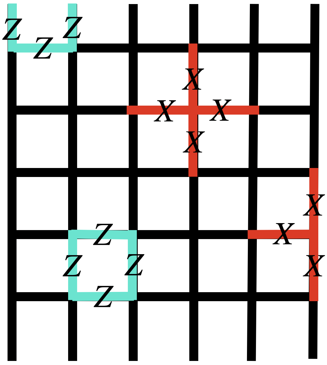
Since our goal is to implement the circuit in Fig. 5 in constant time, we must understand whether the gates that appear in this circuit diagram can be implemented in constant time on the surface code. We shall see towards the end of this section that preparation of an analogue of the state (as opposed to the exact state over the logical qubits) and measurement in the -basis can be done in constant time. So let us focus instead on whether we can implement the unitary gates in Eq. (21).
Because the surface code is a CSS code, it allows for a straightforward implementation of a transversal CNOT gate. Moreover, the CZ gate can be viewed as a CNOT gate conjugated by Hadamards. By folding a surface code in half along its diagonal line, it is possible to implement the logical Hadamard by applying a transversal Hadamard gate on all the qubits followed by a local relabeling of the qubits Moussa 2016 (which builds upon the local unitary equivalence between the the color code and surface code Kubica et al. 2015). We remark that this folding operation is accessible in an interleaved architecture Bombin et al. 2021. Therefore, the CZ gate can also be implemented in constant time. Implementation of can also be done in constant time, either by injecting a eigenstate of the Pauli- operator, or by applying a transversal gate in the folded surface code picture. The transversal gate option, however, requires an extra entangling gate which may adversely affect the threshold and the sub-threshold scaling. On the other hand, the injection requires an additional logical qubit for every logical data qubit, incurring up to a increase in the footprint.
Fortunately, it is possible to have the best of both worlds. Below, we explain a method to modify Eq. (21) so that one does not need to apply the gate explicitly. The price we have to pay is modest; we only need two additional logical qubits, one that keeps the eigenstate of and another one dedicated to increasing the size of the state to .
The key idea is to not apply the explicitly, but instead update the observable that needs to be measured. In this case, the Pauli string simply becomes a tensor product of s and s. In the surface code, measurement in the basis is easy, but measurement in the -basis is less straightforward; the former can be done in constant time, but to the best of our knowledge, measurement in the basis requires an implementation of a single-qubit Clifford gate such as or . However, this Pauli string (say ), up to the stabilizer of the state, is “almost” equal to a Pauli string consisting purely of s. An important observation is that the state obeys the following stabilizer constraint, both before and after the gates in Eq. (21) are applied:
| (23) |
for all . Therefore, if has an even number of s,
| (24) |
where is the number of s in . If , up to a phase, the joint parity of can be measured by measuring all the qubits in the -basis, an operation that can be performed in constant time. If is odd, then there will be one leftover . In that case, one can apply the gate corresponding to the case for the ’th data qubit, which will be initialized to the eigenstate of . This makes the last Pauli in equal to , making even. Moreover, the eigenstate of is returned to its original state after this process, which can be reused later; see Fig. 7 for an example.
Therefore, we have seen that one can perform a PPM using a single state and a eigenstate of , as well as CNOT, CZ, and measurement in the -basis. Once the eigenstate of is prepared at the beginning of the computation, if the state can be prepared in constant time, every operation discussed so far can be done in constant time. Next, we explain how the state preparation can be carried out, thus completing the description of our protocol.
Naïvely, preparation of the state seems to require time. A straightforward way to do this is to initialize all the logical qubits in the state on a one-dimensional array and measure the joint parity of . While the first step requires constant time, the second step requires time if we insist on interacting the surface code patches only via their boundary, using lattice surgery Horsman et al. 2012.
However, for our purposes, it is possible to get away with preparing the state over a long surface code patch; see Fig. 8. Of course, this long surface code patch is not exactly the state. However, they are equivalent up to a Pauli- measurement along the qubits that connect the neighboring patches. Upon measuring these qubits, one must eventually apply a correction.


These partial measurements by themselves do not seem to make the preparation of the state fault-tolerant. However, used in conjunction with the final -basis measurements on the remaining qubits in the ancilla block, we can measure the Pauli Product operator fault-tolerantly. This can be seen by inspecting the stabilizer generators with support strictly on the ancilla block after applying the gates described above in D.3. One can verify that these include all the star operators of the long ancilla block. Moreover, while the errors will undoubtedly spread from the data block, they will spread in a local manner thanks to the transversal nature of the gates used. Therefore, the standard argument in surface code-based error correction Dennis et al. 2002 implies that one can simply measure the entire ancilla block in the -basis and decode, thus fault-tolerantly extracting the measurement outcome of the logical operator of the long ancilla block. This measurement outcome is precisely the PPM. Since the preparation of the state on the long ancilla block can be performed in time, by the discussion in D.3, we conclude that it is possible to perform a -time fault-tolerant PPM.
To summarize, we have shown that an arbitrary fault-tolerant PPM can be performed in constant time. Moreover, all of these operations can be implemented on a planar architecture, involving two folded layers of surface code patches that are superimposed together; see Fig. 9.


Injection of distilled magic states can be implemented by simply increasing the number of logical qubits in the data and the ancilla blocks. Specifically, suppose we can create states in a single logical clock cycle. It will suffice to add extra logical qubits in the data and the ancilla block and store the magic states in the newly allotted qubits in the data block. Since the number of magic state factories is typically much smaller than the number of logical qubits, this additive overhead is expected to be small. Moreover, the magic state factories can be spaced out sufficiently far apart from each other to avoid any routing issues. In the regime studied in this paper, once the number of magic state factories exceeds , the gain from having an extra magic state factory is expected to be insignificant. Since the smallest number of logical qubits needed exceeds a few thousand, we can take the average spacing between the magic state factories to be at least a few hundred, enough room to have independent magic state factories that do not interfere with each other. Of course, one may opt to use more sophisticated distillation protocols that generate multiple magic states at the same time Bravyi and Haah 2012; Haah et al. 2018; Haah et al. 2017; Haah and Hastings 2018. In those cases, the extra logical qubits will need to be physically close to each other.
One may worry that assigning a fixed location for the magic states will cause a routing problem; as we explain below, this is not the case. Thanks to the fact that we can apply arbitrary PPMs, the location of the magic states does not matter.
D.4 Compilation and Execution
We now explain how the newly introduced PPM can be used in practice to compile a quantum algorithm. What we describe below mostly follows from Litinski’s observations Litinski 2019a. Suppose we are given a description of a quantum circuit in terms of Clifford and T-gates. One can, without loss of generality, rewrite this circuit as a sequence of gates of the following form:
| (25) |
where is a Pauli operator, followed by Cliffords and single-qubit measurements. Instead of applying the Cliffords directly, one can simply replace the single-qubit measurements by PPMs. Moreover, Litinski showed that a gate in Eq. (25) can be implemented by consuming a single state and a PPM, followed by a Clifford correction. Therefore, an arbitrary quantum computation can be expressed as a sequence of PPMs on states and a data block, followed by a Clifford correction.
In fact, it is possible to remove the need to apply the Clifford correction entirely. The idea is to dynamically update the gates used in the circuit. Without loss of generality, suppose we have converted the circuit in the form described above, namely, as a sequence of PPMs followed by Clifford corrections of the following form:
| (26) |
for some , where is the Pauli being measured. One can view this as a low-level instruction to the fault-tolerant quantum computer. Given such an instruction, we can execute the circuit on a quantum computer in the following way.
Define the Clifford frame, which is a lookup table of size , where is the number of qubits in the circuit. The Clifford frame is similar to the tableau first introduced by Aaronson and Gottesman Aaronson and Gottesman 2004 and is a compact representation of a Clifford gate. Since the Clifford group generates an automorphism on the Paulis, it suffices to specify their action on the generators, which we choose to be and for , each representing the logical - and -operators of each surface code patch. It is convenient to view the Clifford frame as a table that tells us how to convert each PPM and Clifford correction based on the Clifford corrections that precede them. Specifically, let and be the ’th Pauli operator appearing in the instruction. The Clifford frame converts these Paulis in the following way,
| (27) |
where and and similarly for . The Clifford frame table contains this data; see Table 9 for an example.
| 1 | 0 | 0 | 0 | 0 | 0 | ||
| 1 | 1 | 0 | 1 | 0 | 0 | ||
| 0 | 0 | 1 | 0 | 0 | 0 | ||
| 1 | 0 | 0 | 1 | 0 | 0 | ||
| 0 | 1 | 0 | 0 | 0 | 0 | ||
| 0 | 0 | 0 | 0 | 0 | 1 |
When executing a quantum circuit, the instruction will remain as is, but the Clifford frame will change dynamically. In the beginning, the Clifford frame will be initialized such that
| (28) | |||
In this very first step, we will have a PPM, which can be implemented using either the procedure described above or the one in Ref. Litinski 2019a. Then, suppose the result of the PPM indicates that a Clifford update must be carried out. Instead of applying this Clifford, say , we can update all the remaining PPMs and Clifford corrections by updating the Pauli that underlies them as
| (29) |
However, the instruction set for practical quantum algorithms will be lower bounded by the number of T-gates used, which is often on the order of at least even for state-of-the-art algorithms von Burg et al. 2020; Lee et al. 2020. Updating every gate appearing afterwards will lead to a number of updates of order , which is a significant amount of computation even for a modern computer. Therefore, this is an unwieldy approach. Instead, it is better to update the table such as in Table 9. This amounts to updating and for every .
Happily, such a calculation is extremely simple. For instance, given a , if it commutes with the Pauli operator appearing in the correcting Clifford defined in Eq. (26), no update is needed. Checking the commutation relation only requires number of bitwise operations and parity calculations for -bit strings. If they do not commute, is updated as up to a phase. Both the phase and the updated Pauli can also be computed using number of bitwise operations and parity calculations for -bit strings. Thus, the amount of classical computation scales as parity calculations and bitwise-operations over -bit strings.
Let us emphasize that this calculation can be trivially parallelized to parity calculations and bit-wise operations distributed over processors. Moreover, modern CPUs can perform such operations over thousands of bits on the order of nanoseconds. Therefore, we do not expect the update of the Clifford frame to be a significant bottleneck for the computation.
D.5 Speedups
At first, one may think that a sequence of PPMs can be implemented in time, independent of whether they commute with each other. While we cannot completely discount this possibility, we will demand the sequence of PPMs to satisfy an important constraint. If we were to implement PPMs in a single logical clock cycle, we demand all the Paulis that underlie the PPMs to commute with each other.
If they do not, we encounter the following difficulty. Decoding a logical qubit requires syndrome measurement outcomes in a block, where the last factor of comes from time Dennis et al. 2002. Upon collecting all of these measurement outcomes and decoding, one must apply a correction operation. If certain layers of the block undergo the transversal gates described above, the measurement outcome of the ancilla block may, depending on the outcome of the decoding, have to be retroactively changed. Doing so would necessitate a change in the PPM outcome that occurred in the past, which would in turn signal that a Clifford correction in Eq. (26) was applied incorrectly, resulting in an incorrectly-updated Clifford frame. The incorrect Clifford frame may have triggered an incorrect PPM, which may have already happened.
Fortunately, such a problem is moot if the Paulis that underlie the PPMs commute with each other. In that case, the Clifford corrections also commute with the PPMs; see Eq. (26). Therefore, the Clifford corrections do not change the PPMs within that block. One can simply perform all the PPMs and then update the Clifford frame before we move to the next block.
With this constraint in mind, the speedup we can achieve using this approach is limited by the ratio of T-count and T-depth. In our setup we can optimistically expect up to a -fold speedup with a negligible change in the footprint of the device.
Another constraint is the code distance. At best, one can apply PPMs in a single logical clock cycle using our method. The estimated code distance in Section III.3 ranged from to , suggesting that the best-case scenario of a -fold speedup may be attainable. However, note that whether this is possible or not depends on many microscopic details, such as the timescale needed for different physical operations. Moreover, we would like to emphasize that the threshold and the sub-threshold behavior of the code may change when we implement the transversal gates. The exact extent to which we can speed up the computation using our approach can only be determined by carefully inspecting all of these different factors. These studies are beyond the scope of this paper and are left for future work.
Keeping these caveats in mind, we can estimate the optimistic computation time for a single phase estimation for the molecules described below to be on the order of hours for the cc-pVDZ basis set and hours for the cc-pVTZ basis set.
Appendix E Proof for logarithmic depth “Gizens” rotations
Theorem 1.
Let . Define a -layer circuit as
| (30) |
Then the angles can be chosen such that .
Proof.
Proceed by induction. After layers, assume that the circuit applies
| (31) |
where
| (32) |
Then the action of layer is to rotate
| (33) |
Provided that we choose such that , we therefore have that after layers,
| (34) |
For the base case , we require that
| (35) |
which is trivially achieved by the single Gizens rotation with . After layers, the coefficients are
| (36) |
and we have prepared as intended. ∎
References
- Shor (1994) P. W. Shor, Algorithms for quantum computation: discrete logarithms and factoring, in Proceedings 35th Annual Symposium on Foundations of Computer Science (1994) pp. 124–134.
- Pagano et al. (2020) G. Pagano, A. Bapat, P. Becker, K. S. Collins, A. De, P. W. Hess, H. B. Kaplan, A. Kyprianidis, W. L. Tan, C. Baldwin, L. T. Brady, A. Deshpande, F. Liu, S. Jordan, A. V. Gorshkov, and C. Monroe, Quantum approximate optimization of the long-range Ising model with a trapped-ion quantum simulator, Proceedings of the National Academy of Sciences of the United States of America 117, 25396 (2020), arXiv:1906.02700 .
- Feynman (1982) R. P. Feynman, Simulating physics with computers, Int. J. Theor. Phys. 21, 467 (1982).
- Lloyd (1996) S. Lloyd, Universal Quantum Simulators, Science 273, 1073 (1996).
- McArdle et al. (2020) S. McArdle, S. Endo, A. Aspuru-Guzik, S. C. Benjamin, and X. Yuan, Quantum computational chemistry, Rev. Mod. Phys. 92, 015003 (2020).
- Muller and Blume-Kohout (2015) R. P. Muller and R. Blume-Kohout, The Promise of Quantum Simulation, ACS Nano 9, 7738 (2015).
- Jiang et al. (2012) W. Jiang, N. J. DeYonker, J. J. Determan, and A. K. Wilson, Toward Accurate Theoretical Thermochemistry of First Row Transition Metal Complexes, J. Phys. Chem. A 116, 870 (2012).
- Weymuth et al. (2014) T. Weymuth, E. P. A. Couzijn, P. Chen, and M. Reiher, New Benchmark Set of Transition-Metal Coordination Reactions for the Assessment of Density Functionals, J. Chem. Theory Comput. 10, 3092 (2014).
- Poulin et al. (2014) D. Poulin, M. B. Hastings, D. Wecker, N. Wiebe, A. C. Doherty, and M. Troyer, The Trotter Step Size Required for Accurate Quantum Simulation of Quantum Chemistry, (2014), arXiv:1406.4920 .
- Reiher et al. (2017) M. Reiher, N. Wiebe, K. M. Svore, D. Wecker, and M. Troyer, Elucidating reaction mechanisms on quantum computers, PNAS 10.1073/pnas.1619152114 (2017).
- Babbush et al. (2018) R. Babbush, C. M. Gidney, D. W. Berry, N. Wiebe, J. McClean, A. Paler, A. Fowler, and H. Neven, Encoding Electronic Spectra in Quantum Circuits with Linear T Complexity, Physical Review X 8, 041015 (2018).
- Berry et al. (2019) D. W. Berry, C. Gidney, M. Motta, J. R. McClean, and R. Babbush, Qubitization of Arbitrary Basis Quantum Chemistry Leveraging Sparsity and Low Rank Factorization, Quantum 3, 208 (2019).
- von Burg et al. (2020) V. von Burg, G. H. Low, T. Häner, D. S. Steiger, M. Reiher, M. Roetteler, and M. Troyer, Quantum computing enhanced computational catalysis (2020), arXiv:2007.14460 [quant-ph] .
- Lee et al. (2020) J. Lee, D. W. Berry, C. Gidney, W. J. Huggins, J. R. McClean, N. Wiebe, and R. Babbush, Even more efficient quantum computations of chemistry through tensor hypercontraction (2020), arXiv:2011.03494 [quant-ph] .
- Rice et al. (2021) J. E. Rice, T. P. Gujarati, M. Motta, T. Y. Takeshita, E. Lee, J. A. Latone, and J. M. Garcia, Quantum computation of dominant products in lithium–sulfur batteries, The Journal of Chemical Physics 154, 134115 (2021), https://doi.org/10.1063/5.0044068 .
- Gujarati et al. (2021) T. P. Gujarati, T. Takeshita, A. Hintennach, and E. Lee, A heuristic quantum-classical algorithm for modeling substitutionally disordered binary crystalline materials (2021), arXiv:2004.00957 [quant-ph] .
- Takeshita et al. (2020) T. Takeshita, N. C. Rubin, Z. Jiang, E. Lee, R. Babbush, and J. R. McClean, Increasing the representation accuracy of quantum simulations of chemistry without extra quantum resources, Phys. Rev. X 10, 011004 (2020).
- Su et al. (2021) Y. Su, D. W. Berry, N. Wiebe, N. Rubin, and R. Babbush, Fault-tolerant quantum simulations of chemistry in first quantization (2021), arXiv:2105.12767 [quant-ph] .
- Li et al. (2019) Z. Li, J. Li, N. S. Dattani, C. J. Umrigar, and G. K.-L. Chan, The electronic complexity of the ground-state of the FeMo cofactor of nitrogenase as relevant to quantum simulations, The Journal of Chemical Physics 150, 024302 (2019).
- Bartolucci et al. (2021) S. Bartolucci, P. Birchall, H. Bombin, H. Cable, C. Dawson, M. Gimeno-Segovia, E. Johnston, K. Kieling, N. Nickerson, M. Pant, F. Pastawski, T. Rudolph, and C. Sparrow, Fusion-based quantum computation, (2021), arXiv:2101.09310 .
- Bombin et al. (2021) H. Bombin, I. H. Kim, D. Litinski, N. Nickerson, M. Pant, F. Pastawski, S. Roberts, and T. Rudolph, Interleaving: Modular architectures for fault-tolerant photonic quantum computing, (2021), arXiv:2103.08612 [quant-ph] .
- Browne and Rudolph (2005) D. E. Browne and T. Rudolph, Resource-Efficient Linear Optical Quantum Computation, Phys. Rev. Lett. 95, 010501 (2005).
- Bravyi and Kitaev (2005) S. Bravyi and A. Kitaev, Universal quantum computation with ideal Clifford gates and noisy ancillas, Phys. Rev. A 71, 022316 (2005).
- Gidney and Fowler (2019) C. Gidney and A. G. Fowler, Efficient magic state factories with a catalyzed to transformation, Quantum 3, 135 (2019).
- Litinski (2019a) D. Litinski, A game of surface codes: Large-scale quantum computing with lattice surgery, Quantum 3, 128 (2019a).
- Litinski (2019b) D. Litinski, Magic state distillation: Not as costly as you think, Quantum 3, 205 (2019b).
- Gidney and Ekera (2019) C. Gidney and M. Ekera, How to factor 2048 bit RSA integers in 8 hours using 20 million noisy qubits (2019), arXiv:1905.09749 [quant-ph] .
- Goodenough and Kim (2010) J. B. Goodenough and Y. Kim, Challenges for rechargeable Li batteries, Chemistry of Materials 22, 587 (2010).
- Xu (2004) K. Xu, Nonaqueous liquid electrolytes for lithium-based rechargeable batteries, Chemical Reviews 104, 4303 (2004).
- Weber et al. (2019) R. Weber, M. Genovese, A. J. Louli, S. Hames, C. Martin, I. G. Hill, and J. R. Dahn, Long cycle life and dendrite-free lithium morphology in anode-free lithium pouch cells enabled by a dual-salt liquid electrolyte, Nature Energy 4, 683 (2019).
- Urban et al. (2016) A. Urban, D. H. Seo, and G. Ceder, Computational understanding of Li-ion batteries, npj Computational Materials 2, 10.1038/npjcompumats.2016.2 (2016).
- Wang et al. (2018a) A. Wang, S. Kadam, H. Li, S. Shi, and Y. Qi, Review on modeling of the anode solid electrolyte interphase (SEI) for lithium-ion batteries, npj Computational Materials 4, 10.1038/s41524-018-0064-0 (2018a).
- Zhang (2006) S. S. Zhang, A review on electrolyte additives for lithium-ion batteries, Journal of Power Sources 162, 1379 (2006).
- Im et al. (2017) J. Im, J. Lee, M.-H. Ryou, Y. M. Lee, and K. Y. Cho, Fluorinated Carbonate-Based Electrolyte for High-Voltage Li(Ni 0.5 Mn 0.3 Co 0.2 )O 2 /Graphite Lithium-Ion Battery , Journal of The Electrochemical Society 164, A6381 (2017).
- Pople (1999) J. A. Pople, Nobel lecture: Quantum chemical models, Rev. Mod. Phys. 71, 1267 (1999).
- Perdew et al. (1996) J. P. Perdew, K. Burke, and M. Ernzerhof, Generalized Gradient Approximation Made Simple, Phys. Rev. Lett. 77, 3865 (1996).
- Kresse and Hafner (1993) G. Kresse and J. Hafner, Ab initio molecular dynamics for liquid metals, Phys. Rev. B 47, 558 (1993).
- Kresse and Hafner (1994) G. Kresse and J. Hafner, Ab initio molecular-dynamics simulation of the liquid-metal–amorphous-semiconductor transition in germanium, Phys. Rev. B 49, 14251 (1994).
- Kresse and Furthmüller (1996) G. Kresse and J. Furthmüller, Efficiency of ab-initio total energy calculations for metals and semiconductors using a plane-wave basis set, Comput. Mat. Sci. 6, 15 (1996).
- Kresse and Furthmüller (1996) G. Kresse and J. Furthmüller, Efficient iterative schemes for ab initio total-energy calculations using a plane-wave basis set, Phys. Rev. B 54, 11169 (1996).
- Low and Chuang (2019) G. H. Low and I. L. Chuang, Hamiltonian Simulation by Qubitization, Quantum 3, 163 (2019).
- Kohn (1999) W. Kohn, Nobel lecture: Electronic structure of matter—wave functions and density functionals, Rev. Mod. Phys. 71, 1253 (1999).
- Tubman et al. (2018) N. M. Tubman, C. Mejuto-Zaera, J. M. Epstein, D. Hait, D. S. Levine, W. Huggins, Z. Jiang, J. R. McClean, R. Babbush, M. Head-Gordon, and K. B. Whaley, Postponing the orthogonality catastrophe: efficient state preparation for electronic structure simulations on quantum devices (2018), arXiv:1809.05523 [quant-ph] .
- Horsman et al. (2012) C. Horsman, A. G. Fowler, S. Devitt, and R. V. Meter, Surface code quantum computing by lattice surgery, New Journal of Physics 14, 123011 (2012).
- Łodyga et al. (2015) J. Łodyga, P. Mazurek, A. Grudka, and M. Horodecki, Simple scheme for encoding and decoding a qubit in unknown state for various topological codes, Scientific reports 5, 1 (2015).
- Brown and Roberts (2020) B. J. Brown and S. Roberts, Universal fault-tolerant measurement-based quantum computation, Physical Review Research 2, 033305 (2020).
- Bravyi and Haah (2012) S. Bravyi and J. Haah, Magic-state distillation with low overhead, Phys. Rev. A 86, 052329 (2012).
- Haah et al. (2018) J. Haah, M. B. Hastings, D. Poulin, and D. Wecker, Magic State Distillation at Intermediate Size, Quantum Info. Comput. 18, 114–140 (2018).
- Haah and Hastings (2018) J. Haah and M. B. Hastings, Codes and protocols for distilling , controlled-, and Toffoli gates, Quantum 2, 71 (2018).
- Li (2015) Y. Li, A magic state’s fidelity can be superior to the operations that created it, New Journal of Physics 17, 023037 (2015).
- Haah et al. (2017) J. Haah, M. B. Hastings, D. Poulin, and D. Wecker, Magic state distillation with low space overhead and optimal asymptotic input count, Quantum 1, 31 (2017).
- Górecki et al. (2020) W. Górecki, R. Demkowicz-Dobrzański, H. M. Wiseman, and D. W. Berry, -Corrected Heisenberg Limit, Phys. Rev. Lett. 124, 10.1103/PhysRevLett.124.030501 (2020).
- Kitaev (2003) A. Kitaev, Fault-tolerant quantum computation by anyons, Annals of Physics 303, 2 (2003).
- Bravyi and Kitaev (1998) S. B. Bravyi and A. Y. Kitaev, Quantum codes on a lattice with boundary, (1998), arXiv:quant-ph/9811052 .
- Dennis et al. (2002) E. Dennis, A. Kitaev, A. Landahl, and J. Preskill, Topological quantum memory, Journal of Mathematical Physics 43, 4452 (2002).
- Fowler et al. (2012) A. G. Fowler, M. Mariantoni, J. M. Martinis, and A. N. Cleland, Surface codes: Towards practical large-scale quantum computation, Phys. Rev. A 86, 032324 (2012).
- Paesani et al. (2019) S. Paesani, Y. Ding, R. Santagati, L. Chakhmakhchyan, C. Vigliar, K. Rottwitt, L. K. Oxenløwe, J. Wang, M. G. Thompson, and A. Laing, Generation and sampling of quantum states of light in a silicon chip, Nature Physics 15, 925 (2019).
- Wang et al. (2018b) C. Wang, M. Zhang, X. Chen, M. Bertrand, A. Shams-Ansari, S. Chandrasekhar, P. Winzer, and M. Lončar, Integrated lithium niobate electro-optic modulators operating at cmos-compatible voltages, Nature 562, 101 (2018b).
- Eltes et al. (2020) F. Eltes, G. E. Villarreal-Garcia, D. Caimi, H. Siegwart, A. A. Gentile, A. Hart, P. Stark, G. D. Marshall, M. G. Thompson, J. Barreto, et al., An integrated optical modulator operating at cryogenic temperatures, Nature Materials 19, 1164 (2020).
- Delfosse and Nickerson (2017) N. Delfosse and N. H. Nickerson, Almost-linear time decoding algorithm for topological codes (2017), arXiv:1709.06218 [quant-ph] .
- Kolmogorov (2009) V. Kolmogorov, Blossom V: a new implementation of a minimum cost perfect matching algorithm, Mathematical Programming Computation 1, 43 (2009).
- Fowler (2013) A. G. Fowler, Time-optimal quantum computation (2013), arXiv:1210.4626 [quant-ph] .
- Campbell (2021) E. T. Campbell, Early fault-tolerant simulations of the hubbard model, Quantum Science and Technology 7, 015007 (2021).
- Kivlichan et al. (2020) I. D. Kivlichan, C. Gidney, D. W. Berry, N. Wiebe, J. McClean, W. Sun, Z. Jiang, N. Rubin, A. Fowler, A. Aspuru-Guzik, H. Neven, and R. Babbush, Improved Fault-Tolerant Quantum Simulation of Condensed-Phase Correlated Electrons via Trotterization, Quantum 4, 296 (2020).
- Raussendorf et al. (2003) R. Raussendorf, D. E. Browne, and H. J. Briegel, Measurement-based quantum computation on cluster states, Phys. Rev. A 68, 022312 (2003).
- Raussendorf et al. (2006) R. Raussendorf, J. Harrington, and K. Goyal, A fault-tolerant one-way quantum computer, Annals of physics 321, 2242 (2006).
- Raussendorf et al. (2007) R. Raussendorf, J. Harrington, and K. Goyal, Topological fault-tolerance in cluster state quantum computation, New Journal of Physics 9, 199 (2007).
- Li and Hayashi (2020) M.-J. Li and T. Hayashi, Chapter 1 - Advances in low-loss, large-area, and multicore fibers, in Optical Fiber Telecommunications VII, edited by A. E. Willner (Academic Press, 2020) pp. 3 – 50.
- Childs and Wiebe (2012) A. M. Childs and N. Wiebe, Hamiltonian Simulation Using Linear Combinations of Unitary Operations, Quantum Information and Computation 12, 10.26421/qic12.11-12 (2012).
- Low et al. (2018) G. H. Low, V. Kliuchnikov, and L. Schaeffer, Trading T-gates for dirty qubits in state preparation and unitary synthesis (2018), arXiv:1812.00954 [quant-ph] .
- Wan (2021) K. Wan, Exponentially faster implementations of Select() for fermionic Hamiltonians, Quantum 5, 380 (2021).
- Grover and Rudolph (2002) L. Grover and T. Rudolph, Creating superpositions that correspond to efficiently integrable probability distributions, (2002), arXiv:quant-ph/0208112 .
- Jones (2013) C. Jones, Low-overhead constructions for the fault-tolerant Toffoli gate, Phys. Rev. A 87, 022328 (2013).
- Selinger (2013) P. Selinger, Quantum circuits of -depth one, Physical Review A 87, 10.1103/physreva.87.042302 (2013).
- Campbell and Howard (2017) E. T. Campbell and M. Howard, Unified framework for magic state distillation and multiqubit gate synthesis with reduced resource cost, Physical Review A 95, 10.1103/physreva.95.022316 (2017).
- Gidney (2020) C. Gidney, Quantum block lookahead adders and the wait for magic states (2020), arXiv:2012.01624 [quant-ph] .
- Draper et al. (2006) T. G. Draper, S. A. Kutin, E. M. Rains, and K. M. Svore, A Logarithmic-Depth Quantum Carry-Lookahead Adder, Quantum Info. Comput. 6, 351–369 (2006).
- Chamberland et al. (2020) C. Chamberland, K. Noh, P. Arrangoiz-Arriola, E. T. Campbell, C. T. Hann, J. Iverson, H. Putterman, T. C. Bohdanowicz, S. T. Flammia, A. Keller, G. Refael, J. Preskill, L. Jiang, A. H. Safavi-Naeini, O. Painter, and F. G. S. L. Brandao, Building a fault-tolerant quantum computer using concatenated cat codes, (2020), arXiv:2012.04108 .
- Moussa (2016) J. E. Moussa, Transversal Clifford gates on folded surface codes, Phys. Rev. A 94, 042316 (2016).
- Kubica et al. (2015) A. Kubica, B. Yoshida, and F. Pastawski, Unfolding the color code, New Journal of Physics 17, 083026 (2015).
- Aaronson and Gottesman (2004) S. Aaronson and D. Gottesman, Improved simulation of stabilizer circuits, Phys. Rev. A 70, 052328 (2004).