The Drag Instability in a 2D Isothermal C-shock

Since there is no background structure parallel to the shock front in a 2D plane-parallel, perpendicular shock, no fluid motion is normal to the shock flow. Resultantly, the background states of a 2D perpendicular shock are the same as those in a 1D perpendicular shock. Therefore, a detailed description of the background states can be found in GC20. For clarity, here we simply summarize the shock model to smoothly connect to the linear analysis to be presented later in the paper. We consider the gas flow toward the $+x$ direction across the shock with the magnetic field in the $y$-direction. The equilibrium equations for a plane-parallel shock (i.e. $\partial/\partial t=\partial/\partial y=0$) are derived from Equations(1)–(5), which are given by Equations(6)–(10) in GC20 to provide the background state of our linear analysis in the shock frame. In these equilibrium equations, GC20 also employed a strong coupling approximation under which the ion-neutral drag is balanced by the magnetic pressure gradient of the ions, i.e., $\gamma\rho_{n}L_{B}V_{d}=V_{A,i}^{2}$ where $L_{B}\equiv(-d\ln B/dx)^{-1}$ and $V_{A,i}$ is the Alfvén speed of the ions. Additionally, the equilibrium between cosmic ionization and recombination is assumed; namely, $\beta\rho_{i}^{2}=\xi_{\mathrm{CR}}\rho_{n}$ (see Chen & Ostriker 2012 for justifications of such a choice).

Applying the zero-gradient boundary conditions ($d/dx=0$) far upstream and downstream (i.e., no structures in the steady pre- and post-shock regions), Chen & Ostriker 2012 derived the 1D structure equation of a C-shock. Together with the pre-shock conditions described by $n_{0}$ (neutral number density), $v_{0}=V_{i,0}=V_{n,0}$ (shock velocity), $B_{0}$, and $\chi_{i0}$ (here and throughout this paper, we use the subscript 0 to denote a physical quantity in the pre-shock region), the field compression ratio $r_{B}\equiv B/B_{0}=V_{i,0}/V_{i}$ as well as the neutral compression ratio $r_{n}\equiv\rho_{n}/\rho_{n,0}=V_{n,0}/V_{n}$ can be solved, and $\rho_{i}$, $\rho_{n}$, $B$, $V_{i}$, and $V_{n}$ can be subsequently obtained throughout the shock width. Following GC20, we place the shock front at $x=0$ pc for convenience to plot and refer to shock properties as a function of $x$. In this setup of the problem, the background drift velocity $V_{d}=V_{i}-V_{n}<0$ inside the C-shock (i.e. within the smooth shock transition). As in GC20, we adopt the 1D steady C-shock model shown in Figure 3 of Chen & Ostriker 2012 as the fiducial model for the background state in the shock frame, with the pre-shock parameters $n_{0}=500$ cm^-3, $v_{0}=5$ km/s, $B_{0}=5\mu$G, and $\chi_{i0}=10$. The left panel of Figure 1 shows $r_{n}/r_{B}$ in the fiducial model, which is the same as Figure 1 in GC20.

We now consider the perturbation eigenvector given by $U(\omega,k_{x},k_{y})\equiv(\delta\rho_{i},\delta v_{x,i},\delta v_{y,i},\delta B_{x},\delta B_{y},\delta\rho_{n},\delta v_{x,n},\delta v_{y,n})^{T}$ multiplied by $\exp[\mathrm{i}(k_{x}x+k_{y}y+\omega t)]$ under the WKBJ approximation, where $k_{x}$ is the longitudinal wavenumber, $k_{y}$ is the transverse wavenumber, and $\omega$ is the eigenvalue evaluated in the shock frame. By substituting these perturbations and the background states into the equations (1)–(5), the following linearized equations are obtained (see Gu et al. 2004 and GC20 in the 1D case):

where

Without the loss of generality, we adopt a constant wavenumber $k_{x}$ of $1/0.015$ pc${}^{-1}(\equiv k_{fid}$), as used in GC20. The choice of $k_{x}$ is made to satisfy the WKBJ approximation, as demonstrated in the right panel of Figure 1 where $k_{x}L_{p}$ and $k_{x}L_{B}$ are shown to be all much larger than unity (GC20, also refer to Figure 1 in).

Figure 2 shows the growth rate $\Gamma_{grow}$ ($=$Im[$\omega]<0$, left panel) and its corresponding wave frequency $\omega_{wave}$ ($=$Re[$\omega]$, right panel) of the unstable wave mode as a function of $k_{y}/k_{x}$ in the shock frame, at the location of $x\approx 0.2$ pc in the middle of the C-shock. It is the only unstable mode among all eigenmodes computed from Equation(6). When the longitudinal wavelengths are not exceptionally short (i.e., $k_{x}=k_{fid}$ and $5k_{fid}$ in the figure), the growth rate decreases approximately with increasing $k_{y}/k_{x}$. However, when $k_{x}$ is as large as $20k_{fid}$ (green curve) and $50k_{fid}$ (red curve), the growth rate decreases and even drops to zero, except when $k_{y}/k_{x}$ is sufficiently large in this particular example, which corresponds to a jump of the wave frequency around $k_{y}/k_{x}\gtrsim 12.7$, as shown in the right panel of Figure 2. We explore the underlying physics for the mode properties with simplified dispersion relations in the following subsection.

The eigenvalue problem for Equation(6) amounts to a complicated equation containing a polynomial of $\omega$ to the eighth power. To make the physical analysis of the unstable mode extractable, we attempt to numerically solve Equation(6) by removing as many terms as possible in the matrix $P$ but still obtain the same growth rate and wave frequency as those shown in Figure 2. After this exercise, we realize that Equation(6) can be further reduced to

where $\Gamma_{i}=\mathrm{i}(\omega+k_{x}V_{i})$ is the eigenvalue in the comoving frame of the ions and $\Gamma_{n}=\mathrm{i}(\omega+k_{x}V_{n})$ is the eigenvalue in the comoving frame of the neutrals. Since the collisional rate for an ion with the ambient neutrals $\gamma\rho_{n}$ is tremendously large in a weakly ionized cloud, Equation(17) implies that $\delta v_{i,y}\sim\delta v_{n,y}$, which allows Equation(20) to be further simplified to

and consequently, Equation (16) can be approximated to

The absence of the induction equations for $\delta{\bf B}$ and the momentum equation for $\delta v_{i,x}$ in the above reduced set of linear equations (16)–(20) indicates that the disturbance of the ion flow along the shock direction and that of magnetic fields plays a minor role in the dynamical evolution of the 2D drag instability.

In a 2D perpendicular shock, the linearized equations should approach the 1D result when $k_{y}\ll k_{x}$ (i.e., a transversely large-scale mode). The drag instability can occur in a 1D steady C-shock (GC20). Specifically, for the definite occurrence of the instability in 1D, the rate of the mode $\Gamma_{n}$ observed in the comoving frame of the neutrals is considerably smaller than both the recombination rate $2\beta\rho_{i}$ and the ion-neutral drift rate across a distance of one wavelength (i.e., $k|V_{d}|$), whereas it is considerably larger than the neutral collision rate with the ions (i.e., $\gamma\rho_{i}$) and the sound-crossing rate over one wavelength (i.e., $k_{x}c_{s}$). When the aforementioned conditions are satisfied, the 2D linearized equations (i.e., Equations(18), (19), & (22)) are reduced to those for a 1D perpendicular shock, which yield the simplified dispersion relation (Gu et al. 2004; GC20)

where the positive sign corresponds to a growing wave. As pointed out by GC20, the wave frequency in the shock frame $\omega_{wave}$ is dominated by $k_{x}V_{n}$ instead of the imaginary part of $\Gamma_{n}$ due to the fast background flow across the shock width downstream.

On the other hand, in the regime where $k_{y}\gg k_{x}$ (i.e., a transversely small-scale mode) such that $k_{y}c_{s}$ is much larger than $2\beta\rho_{i}$, $k_{x}V_{i}$, and $k_{x}V_{n}$, Equation(22) suggests that the terms associated with ionization, recombination, and the background shock flows are less significant, revealing a mode with the wave frequency Re[$\omega$]$\approx k_{y}c_{s}$ much larger than Im[$\omega]$. Therefore, Equation(22) suggests the relation $\delta\rho_{i}/\rho_{i}\approx\delta\rho_{n}/\rho_{n}$. In this regime, the in-phase relation between $\delta\rho_{i}$ and $\delta\rho_{n}$ is no longer maintained by the ionization–recombination equilibrium in the regime of a small $k_{y}/k_{x}$ but is a consequence of the fast acoustic wave along the background magnetic fields,¹¹ 1 In comparison, $\delta\rho_{i}/\rho_{i}=(1/2)\delta\rho_{n}/\rho_{n}$ when the ionization–recombination equilibrium is attained. The factor $1/2$ does not appear in this regime when the slow mode is faster than the recombination process. i.e., the so-called slow mode, because $c_{s}<V_{A,n}$ in our fiducial model (Shu 1992, e.g.,). This result, along with Equations(18), (19), and (21), yield the following simplified dispersion relation:

where $k^{2}\equiv k_{x}^{2}+k_{y}^{2}$ and moreover, we have used $\Gamma_{n}^{2}\gamma\rho_{i}\approx k_{y}^{2}c_{s}^{2}\gamma\rho_{i}$ from Equation(22) and $k_{y}c_{s}\gg\sqrt{k_{x}|V_{d}|\gamma\rho_{i}}$ in deriving the above equation. The inequality $k_{y}c_{s}\gg\sqrt{k_{x}|V_{d}|\gamma\rho_{i}}$ holds in the regime where $k_{y}c_{s}\gg 2\beta\rho_{i}$ is being considered here, along with $2\beta\rho_{i}\gg\sqrt{k_{x}|V_{d}|\gamma\rho_{i}}$ in the fiducial model (GC20, see the left panel of Figure 3 in).²² 2 Recall that in a 1D C-shock, $\sqrt{k_{x}|V_{d}|\gamma\rho_{i}}$ is about the growth rate of the drag instability (see Equation 23), which is smaller than $2\beta\rho_{i}$ such that the ionization–recombination equilibrium can be attained for the perturbations to allow the instability to occur.

The positive sign of Equation(24) corresponds to a growing wave with the growth rate related to the ion-neutral drag and the wave frequency $k_{y}c_{s}$ associated with the slow mode. More specifically, in the comoving frame of the neutrals, the phase velocity of the unstable wave is about $-k_{y}c_{s}/k_{x}\hat{x}-c_{s}\hat{y}$ and the group velocity is approximately $-(k_{x}/k_{y})c_{s}\hat{x}-c_{s}\hat{y}$. Hence, in this regime, while both the phase and signal of the unstable wave propagate mainly along the background field lines at the sound speed, the signal also propagates upstream slowly at a speed much smaller than the sound speed. In the shock frame, the phase velocity of the unstable wave is about $[-k_{y}c_{s}/k_{x}+V_{n}]\hat{x}+[-c_{s}+(k_{x}/k_{y})V_{n}]\hat{y}\approx-k_{y}c_{s}/k_{x}\hat{x}-c_{s}\hat{y}$.

Based on the above simplified dispersion relations for unstable modes on different transverse scales, we may be able to interpret the results illustrated in Figure 2. When $k_{y}/k_{x}\rightarrow 0$, both the growth rate and wave frequency converge to the 1D result for the drag instability (GC20), as illustrated by the flat curves for $k_{y}/k_{x}<1$ in Figure 2. However, as $k_{y}/k_{x}$ increases, a new property of the growing mode associated with 2D emerges when the acoustic wave along the background field line, i.e. the slow mode, becomes important. This happens when $c_{s}k_{y}\sim k_{x}V_{n}$ as suggested by the transition of the dispersion relation from Equation(23) to Equation(24). Physically, it occurs when the slow-mode rate $c_{s}k_{y}$ introduced by the additional dimension along the background field in the $y$-direction becomes comparable to the shock-crossing rate $k_{x}V_{n}$ in the $x$-axis through the C-shock. Owing to this transition at the large $k_{y}$, the jump of the wave frequency from a negative to a positive value occurs at $k_{y}/k_{x}\sim V_{n}/c_{s}\equiv\hat{k}_{jump}\approx 16.84$ at $x\approx 0.2$ pc, which agrees with the right panel of Figure 2. While we show the value of $\hat{k}_{jump}$ at one particular $x$, the range of $\hat{k}_{jump}$ within a C-shock can be estimated by the pre-shock conditions. The $V_{n}$ decreases from $v_{0}$ at the beginning of a shock to $v_{0}/r_{f}$ at the end of a shock, where $r_{f}$ is the final compression ratio of the neutral density in the post-shock region given approximately by $\sqrt{2}v_{0}/v_{A,n,0}$ (Chen & Ostriker 2012). Hence, $\hat{k}_{jump}$ decreases from $v_{0}/c_{s}$ to $(v_{0}/r_{f})/c_{s}\approx B_{0}/(\sqrt{4\pi\rho_{n,0}}c_{s})$. In our fiducial model, $\hat{k}_{jump}$ changes from about 25 to 3 across the shock width. In the typical environments of star-forming clouds, $v_{0}\sim$ 1-6 km/s, $n_{0}\sim$ 100-1000 1/cm³, $B_{0}\sim 5-10$ $\mu$G, and the temperature is about 10 K (Chen & Ostriker 2012, e.g., see Table 1 in). Therefore, $\hat{k}_{jump}$ can decrease from $\sim$ 10-30 at the beginning of a C-shock to $\sim$ 1.5-5 at the end of a C-shock.

As $k_{y}/k_{x}$ further increases to an even larger value, the behavior of the growing mode follows the dispersion relation described by Equation(24). This is demonstrated in Figure 3, which zooms in to the region where $k_{y}/k_{x}>20$ in Figure 2. The dashed lines present the growth rate Re[$\Gamma_{n}$] (left panel) and the wave frequency Im[$\Gamma_{n}-k_{x}V_{n}$] (right panel) calculated from Equation(24). As $k_{y}/k_{x}$ increases, the exact growth rates of the unstable mode for various $k_{x}$ computed from Equation(6) converge to Re[$\Gamma_{n}$] while the exact wave frequencies $\omega_{wave}$ overlap with Im[$\Gamma_{n}-kV_{n}$] in the entire zoomed-in region. The slow-mode frequency $k_{y}c_{s}$, as illustrated by the dashed-dotted lines, is also plotted for each value of $k_{x}$. As $k_{y}/k_{x}$ increases, the wave frequency $\omega_{wave}$ in all cases converges toward $k_{y}c_{s}$, confirming that the slow mode emerges and predominates on small transverse scales for the drag instability. Note that the positive wave frequency for $k_{y}/k_{x}>\hat{k}_{jump}$ indicates a growing wave propagating upstream within the 2D perpendicular C-shock, in stark contrast to the growing mode for $k_{y}/k_{x}<\hat{k}_{jump}$, which is more dynamically dominated by the wave convected with the downstream flow across the shock width, similar to the result for a 1D C-shock.

In the case of a moderate value of $k_{x}$ (i.e., $k_{x}=k_{fid}$ and $5k_{fid}$), the growth rate decreases almost monotonically with increasing $k_{y}$ when $k_{y}/k_{x}\gtrsim\hat{k}_{jump}$, in an approximate agreement with the trend described by Equation(24). On the other hand, in the regime where $k_{y}/k_{x}<1$, the growth rate is small or nearly zero when $k_{x}$ is large enough (i.e., $k_{x}=50$ and $100k_{fid}$ in Figure 2) for the small-scale gas pressure perturbation along the shock direction to suppress the growth (Gu et al. 2004; GC20). However, a growing mode exists when $k_{y}/k_{x}\gtrsim 12.7$. Its growth rate rises significantly during the wave frequency transition and then declines, according to Equation(24), as $k_{y}/k_{x}$ increases to a large value. We are unable to derive a simple dispersion relation to describe the rise of the growth rate during the wave frequency transition. It is because more terms in Equations(16)–(20) become comparably important and thus cannot be neglected as a proper approximation for deriving Equation(24). Nevertheless, this complexity of the distinct behaviors of the growth rate at the wave frequency transition can be unraveled by studying the phase differences between perturbed quantities, which will be presented in the next subsection.

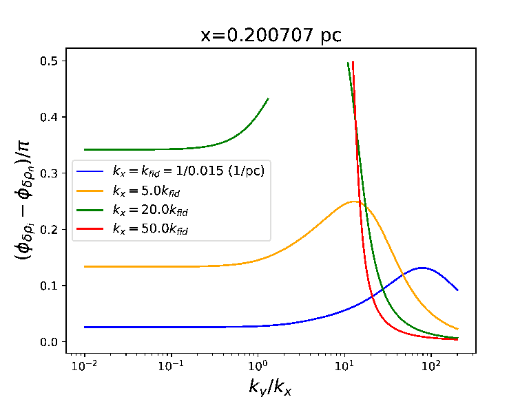
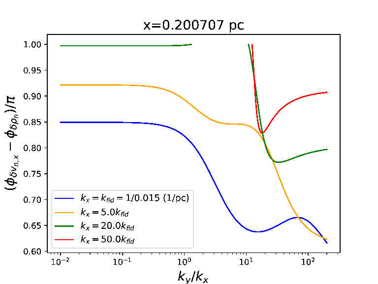
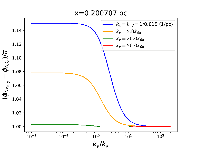
We illustrate the phase differences in Figure 4 corresponding to the growth rate and wave frequency shown in Figure 2. Figure 4 includes the phase difference between the density perturbations, as well as those between the neutral velocity and density perturbations. The flat part of the curves in the range of $k_{y}/k_{x}\lesssim 1$ corresponds to the flat part of the curves in Figure 2, resembling the 1D drag instability for the 2D unstable modes. In contrast to the cases for the small $k_{x}$ (i.e., blue and orange curves), the phase difference between $\delta\rho_{i}$ and $\delta\rho_{n}$ in the cases for the large $k_{x}$ (green and red curves in panel (a) of Figure 4) exhibit a dramatic change when $k_{y}/k_{x}\approx\hat{k}_{jump}=16.8$, corresponding to the jump of the wave frequency. Since the wave frequency of the mode $\omega_{wave}$ is small around this jump transition, the Doppler-shift frequency $k_{x}V_{i}$ with a large $k_{x}$ becomes nonnegligible compared to the ionization rate in the continuity equation of the ions. Consequently, the phase difference between the ion and neutral density perturbations does not stay small by the ionization–recombination equilibrium but becomes large. The phase difference decreases steeply with increasing $k_{y}/k_{x}$ because the rate of the mode is predominated quickly by the slow mode $\approx k_{y}c_{s}$, resulting in the small phase difference between the ion and neutral density perturbations for a large $k_{y}/k_{x}$. It is in accordance with the result that $\delta\rho_{i}/\rho_{i}\approx\delta\rho_{n}/\rho_{n}$ when deriving Equation(24).

The drastic change in $\phi_{\delta\rho_{i}}-\phi_{\delta\rho_{n}}$ also causes the steep change in $\phi_{\delta v_{n,x}}-\phi_{\delta\rho_{n}}$ from $\pi$ to $\approx 0.8\pi$ around the frequency transition (see the green and red curves in panel (b) of Figure 4) through the linearized continuity and momentum equations, leading to a bump in the growth rate of the drag instability near the frequency transition, as shown in the left panel of Figure 2.³³ 3 Recall that the drag instability in a 1D case is driven by the canonical phase difference $3\pi/4$ between $\phi_{\delta v_{n,x}}$ and $\phi_{\delta\rho_{n}}$ (Gu et al. 2004; GC20). Since an acoustic mode can be characterized by the phase difference $\pi$ between density and velocity perturbations, the nearly out-of-phase difference between $\delta v_{n,y}$ and $\delta\rho_{n}$ shown in panel (c) of Figure 4 for $k_{y}/k_{x}\gtrsim 16.8$ reconfirms the right panel of Figure 3, i.e., the emergence of the slow mode when $k_{y}/k_{x}\gtrsim\hat{k}_{jump}$. It also agrees with Equation(21) on the relation $\Gamma_{n}\sim\mathrm{i}k_{y}c_{s}$ for $k_{y}/k_{x}>\hat{k}_{jump}$, which leads to $\delta\rho_{n}/\rho_{n}\sim-\delta v_{n,y}/c_{s}$, i.e., out of phase between $\delta\rho_{n}$ and $\delta v_{n,y}$ for a slow mode.

It was shown by GC20 that the growth of the drag instability in a 1D perpendicular shock is limited by the short time span for an unstable wave to stay within a C-shock as the wave is convected downstream by a fast flow across the shock; specifically, the local growth rate $\Gamma_{grow}$ is much smaller than the wave frequency in the shock frame $\omega_{wave}$. Consequently, a stronger shock with a larger shock width favors a more appreciable growth of the 1D drag instability in the typical environments of star-forming clouds investigated by the authors. However, for a 2D perpendicular shock, as has been studied in the preceding subsection, the transition of the wave frequency from a negative to a positive value allows for the presence of a slowly traveling mode with an arbitrarily small wave frequency in the shock frame when $k_{y}/k_{x}\sim\hat{k}_{jump}$, thereby allowing a tremendous amount of time for the growth of the drag instability within a shock width in this transition regime.

We investigate this expectation by simply considering a mode with a small wave frequency $\omega_{wave}=-10^{-14}$ 1/s $\ll$ the flow crossing time over one longitudinal wavelength $k_{x}V_{n}$. According to the eigenvalue problem, a family of unstable modes should exist with the proper combination of the wavenumbers $k_{x}$ and $k_{y}$ as a function of $x$. For the purpose of computational convenience without loss of generality, we first consider the uniform $k_{x}$ given by the fiducial wavenumber $k_{x}=k_{fid}=$ 1/(0.015 pc), while allowing the $k_{y}$ of the mode to vary with $x$. The results are shown in Figure 5. The resulting growth rate $\Gamma_{grow}$ is indeed larger than $\omega_{wave}$ in most of the region within the C-shock, as illustrated in the left panel of Figure 5. The corresponding profile of $k_{y}/k_{x}$ decreases from 25 to 3 with increasing $x$, in agreement with the transition wavenumber ratio $k_{y}/k_{x}\approx\hat{k}_{jump}=V_{n}/c_{s}$, where $V_{n}$ decreases across the shock width due to density compression, as has been explained in Section II.2. Next, we consider the uniform $k_{y}$ given by $15k_{fid}$ (i.e. a transversely small-scale mode) while allowing the $k_{x}$ of the mode to vary with $x$. The results of the growth rate and wave frequency are considerably similar to those shown in Figure 5, affirming the slow propagation of the unstable modes with $k_{y}/k_{x}\approx\hat{k}_{jump}$ in a 2D perpendicular C-shock. We also study the “counterpart” mode with the small positive wave frequency $\omega_{wave}=10^{-14}$ 1/s for the same case of either the uniform $k_{x}$ or uniform $k_{y}$. We find that the profiles of the growth rate and $k_{y}/k_{x}$ are almost identical to those presented in Figure 5, except that the unstable wave slowly propagates upstream rather than downstream due to the sign change of $\omega_{wave}$.

As the unstable wave propagates slowly at the phase velocity $v_{ph,x}$, the unstable mode is nearly comoving with the shock during the cloud lifetime, which is typically about tens of millions of years (Engargiola et al. 2003; Blitz et al. 2007; Kawamura et al. 2009; Murray 2011; Miura et al. 2012; Meidt et al. 2015; Jeffreson & Kruijssen 2018). Consequently, the MTG is no longer a proper measure for the growth of the slowly propagating modes in the shock frame. For instance, it takes about 82 million years for the unstable mode that we have considered with $\omega_{wave}=-10^{-14}$ 1/s and uniform $k_{x}=k_{fid}$ to travel across the entire shock width,⁴⁴ 4 The wave-crossing time through the shock width is given by $\int_{\rm shock\ width}dx/|v_{ph,x}|=\int dx/(|\omega_{wave}|/k_{x})$. which is $\gtrsim$ the cloud lifetime. It is evident from Figure 2 that there are modes that are almost/exactly stationary in the shock frame (i.e., $\omega_{wave}\approx 0$) and have $\Gamma_{grow}\sim 10^{-13}$ 1/s $\sim 1/0.3$ 1/Myr. Hence, the growth of these modes is approximately given by $\exp(\Gamma_{grow}t)$, which can be substantially larger than unity if $t$ is some fraction of the cloud lifetime. In contrast, the maximum growth of the unstable mode in the 1D case is limited by the shock width and thus is given by MTG, which is merely about 9.9 in the fiducial model (GC20). The 2D mode ought to grow to a nonlinear phase according to the expectation from the linear theory.

Figure 6 shows the amplitude of perturbations for the unstable mode presented in Figure 5. The perturbed quantities are normalized by the $y$-component of the magnetic field perturbation $|\delta B_{y}|/B$. It is evident from the figure that within the shock width where the unstable mode exists, the density perturbations $\delta\rho_{n}/\rho_{n}$ and $\delta\rho_{i}/\rho_{i}$ dominate over the others, implying that the growth of density perturbations plays a decisive role in the dynamical evolution of the instability. Although this outcome of promoting the local density growth of a wave turns out to be the same as that in the 1D case (GC20), the drag instability is coupled with the slow mode in the regime $k_{y}/k_{x}>\hat{k}_{jump}$ for a 2D perpendicular shock, as described in the previous section. This can also be realized from Figure 6, which shows $|\delta v_{n,y}|\gg|\delta v_{n,x}|$ and $|\delta v_{i,y}|\gg|\delta v_{i,x}|$ as a result of the presence of the slow mode propagating along the background magnetic fields in the $y$-direction.

It is worth noting that $\delta B_{x}$ and $\delta B_{y}$ are generated from $B$ due to the gradients of the longitudinal motion $\partial_{y}(\delta v_{i,x})$ (i.e., magnetic wiggling) and $\partial_{x}(\delta v_{i,x})$ (i.e., magnetic compression), respectively, through the induction equation such that $|\delta B_{x}|/|\delta B_{y}|=k_{y}/k_{x}$, in agreement with the ratios $|\delta B_{x}|/|\delta B_{y}|$ in Figure 6 and $k_{y}/k_{x}$ in the right panel of Figure 5. However, given their small amplitudes, magnetic field perturbations simply grow passively through the induction equation and do not play any significant role in the dynamics of the drag instability, confirming that the absence of the induction equation in the reduced set of linearized equations from Equations(16)–(20) still leads to the same growth rate and wave frequency of the drag instability. Finally, as a reminder, in the transversely large-scale regime where $k_{y}/k_{x}\ll V_{n}/c_{s}=\hat{k}_{jump}$ , the property of the drag instability in 2D resembles that in 1D, according to the analysis in the previous subsection. Therefore, the density growth also governs the dynamics of the drag instability for the transversely large-scale mode (GC20).

When $k_{y}/k_{x}\lesssim V_{n}/c_{s}\equiv\hat{k}_{jump}$ (i.e., transversely large-scale modes), the drag instability behaves similarly between 1D and 2D perpendicular C-shocks. When $k_{y}/k_{x}\gtrsim\hat{k}_{jump}$ (i.e., transversely small-scale modes), a new property of the growing mode emerges for 2D perpendicular C-shocks even for a large $k_{x}$, resulting from the ion-neutral drag coupled with the slow mode along the background magnetic field. When $k_{y}/k_{x}\sim\hat{k}_{jump}$, the sign transition of wave frequency occurs. This leads to an unstable mode of a small wave frequency and thus enables a slowly propagating mode to grow substantially within a C-shock, unlimited by the shock width. The linear result suggests that the density growth dominates the evolution of the perturbation growth driven by the drag instability for the modes on both transversely large and small scales.

In this section, we study the local stability of a 2D steady oblique shock in which magnetic fields are not normal to the shock flow. We adopt the background states constructed by Chen & Ostriker 2012. That is, the pre-shock flow is still along the $x$-direction, the shock front in the $y$-$z$ plane, and the pre-shock magnetic field in the $x$-$y$ plane (${\bf B_{0}}=B_{x,0}{\hat{x}}+B_{y,0}{\hat{y}}$), at an initial oblique angle $\theta_{0}$ to the inflow ($B_{y,0}/B_{x,0}=\tan\theta_{0}$). For a steady, parallel-plane oblique shock (i.e., $\partial_{t}=\partial_{y}=\partial_{z}=0$), Chen & Ostriker 2012 derived the equilibrium equations for $r_{n}\equiv\rho_{n}/\rho_{n,0}=v_{0}/V_{n,x}$, $r_{B}\equiv B_{y}/B_{y,0}$ ($B_{x}$ is constant because $\nabla\cdot{\bf B}=0$), and $r_{ix}\equiv v_{0}/V_{i,x}$ from Equations(1)-(5) based on the strong coupling approximation and ionization–recombination equilibrium. Note that $r_{B}$ is not equal to $r_{ix}$ for an oblique shock. By solving the equilibrium equations with a set of pre-shock conditions, the background states including $\rho_{i}$, $\rho_{n}$, $V_{i,x}$, $V_{n,x}$, $V_{i,y}$, $V_{n,y}$, and $B_{y}$ can be subsequently obtained as a function of $x$ within the shock and post-shock regions. Since the field line is not perpendicular to the incoming shock flow, both the field line and gas inflow will continuously change their directions relative to their initial direction as they move across the shock width until they reach the post-shock region (see Figure 7 in the case of the pre-shock conditions given by the fiducial model). As expected, $\bf B$ and $\bf V_{i}$ are first tilted toward the shock front (i.e. a large oblique angle shown in Figure 7) due to the earlier compression of $\rho_{i}$, followed by the subsequent tilt of $\bf V_{n}$ toward the shock front due to the later compression of $\rho_{n}$ within the shock. Finally, ${\bf V_{i}}={\bf V_{n}}$ in the post-shock region as in the pre-shock region, but with a final nonzero oblique angle. The shock width is given by the region between the pre- and post-shock. It is evident from Figure 7 that as $\theta_{0}$ decreases, the compression ratio increases and shock width decreases. Besides, $\bf B$ in the three cases of $\theta_{0}$ shown in Figure 7 all quickly becomes more or less normal to the shock flow by shock compression. All of these results are anticipated from the analysis in Chen & Ostriker 2012.

With the background states, the linearized equations are given by

where

where $V_{A,i}$ is still defined as $B_{y}^{2}/4\pi\rho_{i}$ in terms of the field component parallel to the shock front, which follows the same definition in the case of the 2D perpendicular shock. When the $x$-component of the pre-shock $B$ field is zero, $B_{x}=0$, $V_{i,y}=0$, and $V_{n,y}=0$ (thus $V_{d,y}=0$) throughout the shock. Thus, the matrix $O$ in the above equation for an oblique shock is reduced to the matrix $P$ in equation(6) for a perpendicular shock.

We solve the above eigenvalue problem for the fiducial model of the C-shock with a pre-shock oblique angle $\theta_{0}<90^{\circ}$. As in the perpendicular shock, we find that there is one unstable mode among the eight eigenmodes within a C-shock. Figure 8 shows the growth rate $\Gamma_{grow}$ and wave frequency in the shock frame $\omega_{wave}$ of the unstable mode as a function of $k_{y}/k_{x}$ in the case of $\theta_{0}=45^{\circ}$ with four values of $k_{x}$ at $x\approx 0.2$ pc, approximately in the middle of the oblique C-shock. The figure exhibits two clear general features. First of all, the growth rates and wave frequencies do not vary significantly but have values similar to the case of $k_{y}=0$ in the range of $k_{y}/k_{x}<1$, as shown by the flat part of the curves. The second feature is that regardless of the difference in $k_{x}$, the growth rates of the unstable mode all drop to zero when $k_{y}/k_{x}\approx 9.3$, and the corresponding wave frequencies exhibit a discontinuity at the same wavenumber ratio, which turns out to be exactly equal to $|V_{d,x}|/V_{d,y}$ at $x\approx 0.2$ pc in the fiducial model. We investigate the reason in the next subsections.

Since $V_{n,y}$ and $V_{i,y}$ other than $V_{n,x}$ and $V_{i,x}$ are present in an oblique shock, the Doppler-shift rates in the comoving frame of the ions $\Gamma_{i}$ and neutrals $\Gamma_{n}$ are expressed by $\mathrm{i}(\omega+k_{x}V_{i,x}+k_{y}V_{i,y})$ and $\mathrm{i}(\omega+k_{x}V_{n,x}+k_{y}V_{n,y})$, respectively. Following the same approach in Section II.2 for perpendicular shocks, we focus on the particular mode with $\Gamma_{n}$ smaller than $2\beta\rho_{i}$ and $kV_{d}$ but larger than $\gamma\rho_{i}$. The linear equations expressed in Equation(25) may be reduced to the same set of Equations(18), (19), (21), and (22), except that the additional drag term $\gamma V_{d,y}\delta\rho_{i}$ appears in the $y$-component of the momentum equation for the neutrals, namely (cf. Equation(21)):

Moreover, as the recombination rate $2\beta\rho_{i}>\Gamma_{n}$ for this mode, Equation(22) is reduced to $\delta\rho_{i}/\rho_{i}\approx(1/2)\delta\rho_{n}/\rho_{n}$ due to the ionization equilibrium. The resulting dispersion reads

In the regime where $k_{y}/k_{x}\ll 1$ and $\Gamma_{n}>k_{x}c_{s}$, the above equation is reduced to Equation(23), the typical growth rate and wave frequency for the 1D drag instability (Gu et al. 2004; GC20), but with a background state for an oblique shock. As in the case of a 2D perpendicular shock discussed in the preceding section, this mode behavior of an oblique shock is consistent with the flat part of the curves for both growth rate and wave frequency in Figure 8. As $k_{y}/k_{x}$ increases to the moderate value $|V_{d,x}|/V_{d,y}\equiv\hat{k}_{discon}=9.3$, Figure 8 shows that the growth rates decline and become zero around $\hat{k}_{discon}$. Besides, the corresponding wave frequencies decrease gradually with increasing $k_{y}/k_{x}$ and then abruptly drop around $\hat{k}_{discon}$. This behavior of the growth rate and wave frequency can be understood in terms of Equation(45), which admits a special solution Re$[\Gamma_{n}]=0$ when $k_{x}V_{d,x}+k_{y}V_{d,y}=0$. The dynamics attributed to the absence of the growing mode at $k_{y}/k_{x}=\hat{k}_{discon}$ is that the drag force in the $x$-direction (i.e., $\gamma V_{d,x}\delta\rho_{i}$) acts out of phase with the drag force in the $y$-direction for the neutrals (i.e., $\gamma V_{d,y}\delta\rho_{i}$), therefore suppressing the density enhancement in the neutral continuity equation and thus quenching the drag instability.

To explain the property of the wave frequency shown in the right panel of Figure 8, we investigate the behavior of Equation(45) near $k_{y}/k_{x}=\hat{k}_{discon}$. Because $kc_{x}\gg k_{x}V_{d,x}+k_{y}V_{d,y}\approx 0$ around this wavenumber ratio, the dispersion relation of the unstable mode described by Equation(45) is simplified to

where the plus (minus) sign of the imaginary part of the above expression (i.e., the wave frequency in the comoving frame of the neutrals) is taken when $k_{x}V_{d,x}+k_{y}V_{d,y}<0$ ($>0$). Due to this sign change, the wave frequency in the shock frame $\omega_{wave}$ (=Re[$\omega$]) at $k_{y}/k_{x}=k_{discon}$ exhibits a discontinuity, with the difference given by $\approx 2kc_{s}$. As $k_{y}/k_{x}$ increases beyond $\hat{k}_{discon}$ for a given $k_{x}$, Re[$\omega$] ($=-k_{x}V_{n,x}-k_{y}V_{n,y}-kc_{s}$) increases more negatively; approximately speaking, Re[$\omega$]$\approx-k_{y}(V_{n,y}+c_{s})\propto-k_{y}$, in close agreement with the right panel of Figure 8.

References

- André et al. (2014) André, P., Di Francesco, J., Ward-Thompson, D., Inutsuka, S. -I., Pudritz, R. E., Pineda, J. E. 2014, Protostars and Planets VI, Henrik Beuther, Ralf S. Klessen, Cornelis P. Dullemond, and Thomas Henning (eds.), University of Arizona Press, Tucson, 914 pp., p.27-51
- Ballesteros-Paredes et al. (2007) Ballesteros-Paredes, J., Klessen, R. S., Mac Low, M.-M., et al. 2007, Protostars and Planets V, B. Reipurth, D. Jewitt, and K. Keil (eds.), University of Arizona Press, Tucson, 951 pp., p.63-80
- Blitz et al. (2007) Blitz, L., Fukui, Y., Kawamura, A., Leroy, A., Mizuno, N., & Rosolowsky, E., 2007, Protostars and Planets V. Univ. Arizona Press, Tucson, AZ, p. 81
- Chen & Ostriker (2012) Chen, C.-Y, & Ostriker, E. 2012, ApJ, 744, 124
- Chen & Ostriker (2014) Chen, C.-Y, & Ostriker, E. 2014, ApJ, 785, 69 2, ApJ, 567, 947
- Dalgarno (2006) Dalgarno, A. 2006, Proceedings of the National Academy of Science, 103, 12269
- Draine (1980) Draine, B. T. 1980, ApJ, 241, 1021
- Draine & McKee (1993) Draine, B. T., & McKee, C. F. 1993, ARA&A, 31, 373
- Draine et al (1983) Draine, B. T., Roberge, W. G., & Dalgarno, A. 1983, ApJ, 264, 485
- Elmegreen & Scalo (2004) Elmegreen, B. G., & Scalo, J. 2004, Annu. Rev. Astron. Astrophys., 42, 211
- Engargiola et al. (2003) Engargiola, G., Plambeck, R. L., Rosolowsky, E., & Blitz, L., 2003, ApJS, 149, 343
- Falle et al. (2009) Falle, S.A.E.G., Hartquist, T.W., van Loo, S. In: Pogorlov, N.V., Audit, E., Colella, P., Zank, G.P. 2009, (eds.) Numerical Modeling of Space Plasma Flows, p. 80. Astronomical Society of the Pacific
- Flower & Pineau Des Forêts (1998) Flower, D. R., & Pineau Des Forêts, G. 1998, MNRAS, 297, 1182
- Flower & Pineau Des Forêts (2010) Flower, D. R., & Pineau Des Forêts, G. 2010, MNRAS, 406, 1745
- Fukui & Kawamura (2010) Fukui, Y., & Kawamura, A. 2010, ARA&A, 48, 547
- Girichidis et al. (2020) Girichidis, P., Offner, S.S.R., Kritsuk, A.G. et al. 2020, Space Sci Rev, 216, 68
- (17) Gu, P.-G., & Chen, C.-Y. 2020, ApJ, 898, 67 (GC20)
- Gu et al. (2004) Gu, P.-G., Lin, D. N. C., & Vishniac, E. T., Astrophysics & Space Science, 292, 261
- Gusdorf et al. (2008) Gusdorf, A., Cabrit, S., Flower, D. R., et al. 2008, A&A, 482, 809
- Hennebelle & Falgarone (2012) Hennebelle, P., & Falgarone, E. 2012, Astron. Astrophys. Rev., 20, 55
- Hennebelle & Inutsuka (2019) Hennebelle, P., & Inutsuka, S.-I. 2019, Frontiers in Astronomy and Space Sciences, 6, 5
- Hezareh et al. (2010) Hezareh, T., Houde, M., McCoey, C., et al. 2010, ApJ, 720, 603
- Hezareh et al. (2014) Hezareh, T., Csengeri, T., Houde, M., et al. 2014, MNRAS, 438, 663
- Indriolo & McCall (2012) Indriolo, N., & McCall, B. J. 2012, ApJ, 745, 91
- Jeffreson & Kruijssen (2018) Jeffreson, S. M. R. & Kruijssen, J. M. D. 2018, MNRAS, 476, 3688
- Johansen & Youdin (2007) Johansen, A., & Youdin, A. 2007 ApJ, 662, 627
- Kawamura et al. (2009) Kawamura, A. et al., 2009, ApJS, 184, 1
- Kennicutt & Evans (2012) Kennicutt, R. C., & Evans, N. J. 2012, Annu. Rev. Astron. Astrophys. 50, 531
- Könyves et al. (2015) Könyves, V., André, P., Menśhchikov, A., Palmeirim, P., Arzoumanian, D., Schneider, N., et al. 2015, A&A, 584, 91
- Lehmann & Wardle (2016) Lehmann, A., & Wardle, M. 2016, MNRAS, 455, 2066
- Li & Nakamura (2004) Li, Z.-Y., & Nakamura, F. 2004, ApJ, 609. 83
- Li et al. (2014) Li, H.-B., Goodman, A., Sridharan, T. K., et al. 2014, Protostars and Planets VI, 101
- Li & Houde (2008) Li, H.-B., & Houde, M. 2008, ApJ, 677, 1151
- Mac Low (1999) Mac Low, M.-M. 1999, ApJ, 524, 169
- Mac Low et al. (1998) Mac Low, M.-M., Klessen, R. S., Burkert A. et al., 1998, Phys. Rev. Lett. 80, 2754
- McKee et al. (2010) McKee, C. F., Li, P. S., & Klein, R. I. 2010, ApJ, 720, 1612
- Meidt et al. (2015) Meidt, S. E. et al., 2015, ApJ, 806, 72
- Mestel & Spitzer (1956) Mestel, L., & Spitzer, L. 1956, MNRAS, 116, 503
- Miura et al. (2012) Miura, R. E. et al., 2012, ApJ, 761, 37
- Murray (2011) Murray, N., 2011, ApJ, 729, 133
- Nakamura & Li (2005) Nakamura, F., & Li, Z.-Y. 2005, ApJ, 631, 411
- Nakamura & Li (2008) Nakamura, F., & Li, Z.-Y. 2008, ApJ, 687, 354
- Polychroni et al. (2013) Polychroni, D., Schisano, E., Elia, D., Roy, A., Molinari, S., Martin, P., et al. 2013, ApJ,777, 33
- Shu (1992) Shu, F. H. 1992, in Physics of Astrophysics, Vol. II, ed. F. H. Shu (Mill Valley, CA: Univ. Science Books)
- Smith & Mac Low (1997) Smith, M. D., & Mac Low, M.-M. 1997, A&A, 326, 801
- Spitzer (1956) Spitzer, L. 1956, Physics of Fully Ionized Gases, New York: Interscience Publishers
- Stone (1997) Stone, J. M. 1997, ApJ, 487, 271
- Stone et al. (1998) Stone, J. M., Ostriker, E. C., Gammie, C. F. 1998, ApJ508, 99
- Tang et al. (2018) Tang, K. S., Li, H.-B., & Lee, W.-K. 2018, ApJ, 862, 42
- Tielens (2005) Tielens, A. G. G. M. 2005, The Physics and Chemistry of the Interstellar Medium, Cambridge, UK: Cambridge University Press
- Valdivia et al. (2017) Valdivia, V., Godard, B., Hennebelle, P., et al. 2017, A&A, 600, A114
- Wardle (1990) Wardle, M. 1990, ApJ, 246, 98
- Wardle (1991) Wardle, M. 1991, MNRAS, 251, 119
- Wardle (1998) Wardle, M. 1998, MNRAS, 298, 507
- Xu & Li (2016) Xu, D., & Li, D. 2016, ApJ, 833, 90
- Zweibel (2015) Zweibel, E. 2015, Ambipolar Diffusion, in Magnetic Fields in Diffuse Media, ed. Alexander Lazarian, Elisabete M. de Gouveia Dal PinoClaudio Melioli, 407, 285