A symmetry on weakly increasing trees and
multiset Schett polynomials

As unified generalization of increasing trees and plane trees, the weakly increasing trees on a multiset were introduced recently in the joint work of the two authors with Ma and Zhou [24]. The objective of this article is to prove both bijectively and algebraically the symmetry of the joint distribution of “even-degree nodes on odd levels” and “odd-degree nodes” on weakly increasing trees. The discovery of this symmetric distribution was inspired by Dumont’s combinatorial interpretation of the Jacobi elliptic functions [15, 16], Deutsch’s combinatorial bijection on plane trees [11] and Liu’s recursive involution on increasing trees [28].

Let us begin with the definition of weakly increasing trees on a multiset. A plane tree $P$ can be defined recursively as follows: a node $v$ is one designated vertex, which is called the root of $P$. Then either $P$ contains only one node $v$, or it has a sequence $(P_{1},P_{2},\ldots,P_{k})$ of $k$ subtrees $P_{i}$, each of which is a plane tree. So, the subtrees of each node are linearly ordered. We write these subtrees in the order left to right when we draw such trees. We also write the root $v$ on the top and draw an edge from $v$ to the root of each of its subtrees. Let $(p_{1},p_{2},\ldots,p_{n})$ be a sequence of positive integers. Denote by $M=M(p_{1},p_{2},\ldots,p_{n})$ the multiset $\{1^{p_{1}},2^{p_{2}},\ldots,n^{p_{n}}\}$ and let $p=\sum_{i=1}^{n}p_{i}$.

Note that weakly increasing trees on $[n]:=\{1,2,\ldots,n\}$ are exactly increasing trees on $[n]$, while weakly increasing trees on $\{1^{n}\}$ are in obvious bijection with plane trees with $n$ edges. This enables us to study the unity between plane trees and increasing trees in the framework of weakly increasing trees. The enumerative results obtained in [24] reflect that weakly increasing trees is a natural and nice generalization of plane trees and increasing trees:

• •

  The number of weakly increasing trees on $M(p_{1},\ldots,p_{n})$ has a compact product formula

  $$|\mathcal{T}_{M}|=\frac{1}{1+N_{n}}\prod_{i=1}^{n}{N_{i}+p_{i}\choose p_{i}},$$

  where $N_{i}:=p_{1}+\cdots+p_{i}$ for each $i\in[n]$.

• •

  The $M$-Eulerian–Narayana polynomial, which interpolates between the Eulerian polynomial (when $M=[n]$) and the Narayana polynomial (when $M=\{1^{n}\}$), was defined by

  (1.1)

  $$A_{M}(t)=\sum_{T\in\mathcal{T}_{M}}t^{\mathsf{leaf}(T)},$$

  where $\mathsf{leaf}(T)$ denotes the number of leaves of $T$. The $\gamma$-positivity of $A_{M}(t)$ has an unified group action proof which possesses an unexpected application in interpreting the $\gamma$-coefficients of the $k$-multiset Eulerian polynomials (see [24] for $k=2$ and [26] for general $k$).

• •

  There are connections between $M$-Eulerian–Narayana polynomials for the multiset $M=\{1^{2},2^{2},\ldots,n^{2}\}$ (resp. $M=\{1^{2},2^{2},\ldots,(n-1)^{2},n\}$) and Savage and Schuster’s ${\bf s}$-Eulerian polynomials for the sequence ${\bf s}=(1,1,3,2,5,3,\ldots,2n-1,n,n+1)$ (resp. ${\bf s}=(1,1,3,2,5,3,\ldots,2n-1,n)$).

In this paper, we continue to investigate the weakly increasing trees by considering several classical tree statistics related to the degrees and levels of nodes. The degree (also called out-degree) of a node in a tree is the number of its children and the level of a node is measured by the number of edges lying on the unique path from the root to it. So the root lies at level $0$. For $T\in\mathcal{T}_{M}$, the six tree statistics on $T$ that we consider are:

• •

  The number of nodes of degree $q$ in $T$, denoted by $\mathsf{deg}_{q}(T)$. In particular, $\mathsf{deg}_{0}(T)=\mathsf{leaf}(T)$.

• •

  The number of nodes of degree $q$ in odd levels of $T$, denoted by $\mathsf{od}_{q}(T)$.

• •

  The number of nodes in even levels of $T$, denoted by $\mathsf{el}(T)$.

• •

  The number of odd-degree nodes in $T$, denoted by $\mathsf{odd}(T)$.

• •

  The number of even-degree nodes in odd (resp. even) levels of $T$, denoted by $\mathsf{oe}(T)$ (resp. $\mathsf{ee}(T)$).

The above six tree statistics have been extensively studied in the literature for plane trees in [6, 9, 10, 11, 18, 32] and for increasing trees in [3, 8, 23, 28]. Particularly, Deutsch [11] introduced a bijection $\widehat{(\,)}$ from the set $\mathcal{P}_{n}$ of plane trees with $n$ edges to itself such that for each $T\in\mathcal{P}_{n}$

Inspired by Deutsch’s result, a natural problem arises: is the above equidistribution still holds on increasing trees or even on weakly increasing trees? The answer to this question is affirmative and it turns out that Deutsch’s bijection $\widehat{(\,)}$ can be extended¹¹ 1 We learn that Shishuo Fu and his master student have also observed such extension independently. to weakly increasing trees.

In fact, Deutsch’s bijection $\widehat{(\,)}$ can be generalized directly to $\widehat{(\,)}=\widehat{(\,)}_{M}:\mathcal{T}_{M}\rightarrow\mathcal{T}_{M}$ by taking the labels of trees into account as follows. The mapping $\widehat{(\,)}$ is defined inductively. Firstly, set $\widehat{\emptyset}=\emptyset$. Let $T$ be a nonempty weakly increasing tree in $\mathcal{T}_{M}$. For any node $v$ of $T$ let $T_{v}$ denote the subtree of $T$ induced by $v$ and its descendants. Clearly, the leftmost child of the root $0$ in $T$ must be a node of label $1$ and let $H$ denote the subtree of $T$ induced by this $1$ and its descendants. Suppose that $u_{1},\ldots,u_{s}$ are all children of the root $0$ other than the leftmost child in $T$ from left to right. We construct the weakly increasing tree $\widehat{T}$ as follows:

• •

  Change the label $1$ of the root of $\widehat{H}$ to $0$ and denote by $\widehat{H}^{*}$ the resulting tree;

• •

  Attach an isolate node $1$ to the root $0$ of $\widehat{H}^{*}$ such that it is the leftmost child of $0$;

• •

  Make $\widehat{T}_{u_{1}},\ldots,\widehat{T}_{u_{s}}$ the branches of the above new node $1$ from left to right.

See Fig. 2 for graphical descriptions of $\widehat{T}$. By induction on the number of edges of the tree, we obtain the following generalization of Deutsch’s result.

Theorem 1.2 is new even for increasing trees, i.e., when $M=[n]$. It reflects again the wonderful unity between plane trees and increasing trees. One interesting consequence of Theorem 1.2 is

which provides a new interpretation of the $M$-Eulerian–Narayana polynomial $A_{M}(t)$ defined by (1.1). This interpretation for the classical Eulerian polynomials in terms of increasing trees was known in [4]. Noticing

another interesting corollary of Theorem 1.2 is the following equidistribution.

On the other hand, Liu [28] constructed recursively an involution on $\mathcal{T}_{n}$, the set of increasing trees on $[n]$, which proves a refined symmetry extension of Corollary 1.3 for $M=[n]$.

It is Corollary 1.3 and Theorem 1.4 that motivates the following refined symmetry distribution for weakly increasing trees.

Our construction of involution $\widetilde{(\,)}$ on weakly increasing trees, having close flavor as Deutsch’s bijection $\widehat{(\,)}$, is essentially different with Liu’s involution $\phi$ on increasing trees. We have no idea how Liu’s involution can be extended to weakly increasing trees.

The Jacobi elliptic function $\mathrm{sn}(u,\alpha)$ may be (see [19]) defined by the inverse of an elliptic integral:

where $\alpha\in(0,1)$ is a real number. The other two functions are given by

The Taylor expansions of $\mathrm{sn}(z,\alpha),\mathrm{cn}(z,\alpha)$ and $\mathrm{dn}(z,\alpha)$ read

Consider the derivative operator on the polynomials in three variables defined by

The polynomial $S_{n}(x,y,z):=D^{n}(x)$ is known as the $n$-th Schett polynomial (according to Dumont [15]) which has the form:

The first values of $S_{n}(x,y,z)$ are:

The main result of Schett [33] was to prove that

• •

  the coefficient of $(-1)^{n}\alpha^{2j}u^{2n+1}/(2n+1)!$ in the Taylor expansion of $\mathrm{sn}(u,\alpha)$ equals $s_{2n,0,j}$ or $s_{2n+1,0,j}$;

• •

  the coefficient of $(-1)^{n}\alpha^{2i}u^{2n}/(2n)!$ (resp. $(-1)^{n}\alpha^{2n-2i}u^{2n}/(2n)!$) in the Taylor expansion of $\mathrm{cn}(u,\alpha)$ (resp. $\mathrm{dn}(u,\alpha)$) equals $s_{2n-1,i,0}$ or $s_{2n,i,0}$.

This indicates that Schett polynomials is a generalization of the Jacobi elliptic functions. Schett also noticed that $S_{m}(1,1,1)=\sum_{i,j\geq 0}s_{m,i,j}=m!$, which inspired Dumont [15, 16] to find the first interpretation of the Schett polynomials in terms of the parity of cycle peaks in permutations. Our consideration of the parity of the degrees and levels of nodes in increasing trees leads to a new interpretation of the Schett polynomials $S_{n}(x,y,z)$.

In view of Theorem 1.6, the joint distribution in (1.2)

is named the multiset Schett polynomial for the multiset $M$, extending the Jacobi elliptic functions from sets to multisets. In particular, we connect the Jacobi elliptic functions for plane trees to fighting fish with a marked tail originally studied by Duchi, Guerrini, Rinaldi and Schaeffer [14].

Gamma-positive polynomials arise frequently in enumerative combinatorics and have recent impetus coming from enumerative geometry; see the two recent surveys by Brändén [5] and by Athanasiadis [2]. A univariate polynomial $f(x)$ of degree $n$ is said to be $\gamma$-positive if it can be expanded as

with $\gamma_{k}\geq 0$. If such an expansion exists, then $f(x)$ is also palindromic (or symmetric) and unimodal. Moreover, the $\gamma$-coefficients $\gamma_{k}$ usually (but not always) have nice combinatorial interpretations, which makes this theme even more charming. The classical Eulerian polynomials, as well as their various generalizations [4, 27, 24], are some of the typical examples arising from permutation statistics.

A bivariate polynomial $h(x,y)$ is said to be homogeneous $\gamma$-positive, if $h(x,y)$ is homogeneous and $h(x,1)$ is $\gamma$-positive. A trivariate polynomial $p(x,y,z)=\sum_{i}x^{i}s_{i}(y,z)$ is partial $\gamma$-positive if every $s_{i}(y,z)$ is homogeneous $\gamma$-positive. There has been recent interest in investigating partial $\gamma$-positive polynomials with combinatorial meanings [29, 30, 25]. Generalizing the symmetry in (1.2), we aim to prove the partial $\gamma$-positivity of the reduced multiset Schett polynomial

Noticing the relationships

we see that the reduced multiset Schett polynomial $\hat{S}_{M}(x,y,z)$ encodes essentially the same information as $S_{M}(x,y,z)$.

The two statistics $\mathsf{act}$ and $\mathsf{eact}$ concerned are defined as follows.

The purpose of this paper is threefold. One is to construct the involution $\widetilde{(\,)},:\mathcal{T}_{M}\rightarrow\mathcal{T}_{M}$ to prove combinatorially the refined symmetry (1.2), which is provided in Section 2, as well as several relevant interesting consequences. The second is to study the algebraic aspect of the refined symmetry (1.2), including proofs of Theorem 1.6 and a conjecture of Ma–Mansour–Wang–Yeh [31] via Chen’s context-free grammar and a generating function proof of (1.2), which are fulfilled in Section 3. The last is to develop a group action on weakly increasing binary trees to prove Theorem 1.7, which forms the content of Section 4. This paper reflects appropriately again (cf. [21]) the deep ideas of our great master, M.P. Schützenberger: every algebraic relation is to be given a combinatorial counterpart and vice versa.

In this section, we construct the involution $\widetilde{(\,)}:\mathcal{T}_{M}\rightarrow\mathcal{T}_{M}$ for Theorem 1.5. It will be defined recursively.

For $M=\emptyset\text{ and }\{1\}$, we let $\widetilde{T}=T$ for any $T\in\mathcal{T}_{M}$. If $M=[2]$ and $\{1^{2}\}$, we let

$T$	$\widetilde{T}$	$T$	$\widetilde{T}$

.

For a general fixed multiset $M$ and $T\in\mathcal{T}_{M}$, we have the decomposition of $T$ (see the left graph of Fig. 3) as:

• •

  The leftmost child of the root $0$ is a node with label $1$. Let $x$ and $y$ be the leftmost child and the closest sibling of this special $1$ in $T$. It is possible that $x$ or $y$ may not exist, which does not affect our construction.

• •

  Let $v_{1},\ldots,v_{s}$ be all the siblings of $x$ from left to right. Denote $F=T_{x}$ the subtree of $T$ induced by $x$ and its descendants.

• •

  Let $u_{1},\ldots,u_{t}$ be all the children of $y$ from left to right. Denote $H$ the subtree of $T$ induced by the root and its children to the right of $y$ together with their descendants.

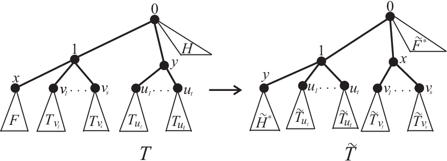
The main idea underling the construction is to exchange the role of $x$ and $y$ and further exchange their siblings with their children. Let us define $\widetilde{T}$ recursively by the following steps (see again Fig. 3 for nice visualization of our involution):

• i)

  Change the label $x$ of the root of $\widehat{F}$ to $0$ and denote by $\widehat{F}^{*}$ the resulting tree;

• ii)

  Attach a node $1$ and a node $x$ at the root $0$ of $\widehat{F}^{*}$ as its first and second children, respectively;

• iii)

  Change the label $0$ of the root of $\widehat{H}$ to $y$ and attach the resulting tree, denoted $\widehat{H}^{*}$, at the node $1$ as its leftmost branch; further attach the subtrees $\widetilde{T}_{u_{1}},\ldots,\widetilde{T}_{u_{t}}$ at the node $1$ as its branches from left to right;

• iv)

  Finally, attach the subtrees $\widetilde{T}_{v_{1}},\ldots,\widetilde{T}_{v_{s}}$ at the node $x$ as its branches from left to right and let the resulting tree be $\widetilde{T}$ (see the right graph in Fig. 3).

For example, for $M=\{1^{2},2^{2}\}$ in Fig. 1, the mapping $\widetilde{(\,)}$ works as $\widetilde{T}_{1}=T_{7},\widetilde{T}_{2}=T_{18},\widetilde{T}_{3}=T_{8},\widetilde{T}_{4}=T_{11},\widetilde{T}_{5}=T_{10},\widetilde{T}_{6}=T_{17},\widetilde{T}_{9}=T_{15},\widetilde{T}_{12}=T_{14}$ and $\widetilde{T}_{13}=T_{16}$. It is clearly from the above construction that $\widetilde{T}$ is a weakly increasing trees in $\mathcal{T}_{M}$ and so the mapping $\widetilde{(\,)}:\mathcal{T}_{M}\rightarrow\mathcal{T}_{M}$ is well-defined. Moreover, this mapping is an involution, as evident from the construction by induction on the size of $M$.

It remains to verify that

Let us first consider the number of odd-degree nodes. We need to distinguish three cases:

1. (1)

   If both $x$ and $y$ exist, then

   	$\displaystyle\mathsf{odd}(T)$	$\displaystyle=\mathsf{odd}(H)+\mathsf{odd}(F)+\sum_{i=0}^{s}\mathsf{odd}(T_{v_{i}})+\sum_{i=0}^{t}\mathsf{odd}(T_{u_{i}})+\chi(\text{$s$ even})+\chi(\text{$t$ odd})$
   		$\displaystyle=\mathsf{oe}(\widetilde{H}^{*})+\mathsf{oe}(\widetilde{F}^{*})+\sum_{i=0}^{s}\mathsf{oe}(\widetilde{T}_{v_{i}})+\sum_{i=0}^{t}\mathsf{oe}(\widetilde{T}_{u_{i}})+\chi(\text{$s$ even})+\chi(\text{$t$ odd})=\mathsf{oe}(\widetilde{T}),$

   where $\chi(\mathsf{S})$ equals $1$, if the statement $\mathsf{S}$ is true; and $0$, otherwise.

2. (2)

   If $x$ does not exist, then

   	$\displaystyle\mathsf{odd}(T)$	$\displaystyle=\mathsf{odd}(H)+\sum_{i=0}^{s}\mathsf{odd}(T_{v_{i}})+\chi(\text{$t$ odd})$
   		$\displaystyle=\mathsf{oe}(\widetilde{H}^{*})+\sum_{i=0}^{t}\mathsf{oe}(\widetilde{T}_{u_{i}})+\chi(\text{$t$ odd})=\mathsf{oe}(\widetilde{T}).$

3. (3)

   If $x$ does not exist, then

   	$\displaystyle\mathsf{odd}(T)$	$\displaystyle=1+\mathsf{odd}(F)+\sum_{i=0}^{s}\mathsf{odd}(T_{v_{i}})+\chi(\text{$s$ even})$
   		$\displaystyle=1+\mathsf{oe}(\widetilde{F}^{*})+\sum_{i=0}^{s}\mathsf{oe}(\widetilde{T}_{v_{i}})+\chi(\text{$s$ even})=\mathsf{oe}(\widetilde{T}).$

In either case, we have

Since $\widetilde{(\,)}$ is an involution, it follows that

also holds. Finally, we need to consider the number of even-degree nodes on even levels:

This finishes the proof that the involution $\widetilde{(\,)}:\mathcal{T}_{M}\rightarrow\mathcal{T}_{M}$ has the feature (2.1) and provides the combinatorial proof of symmetry (1.2).

References

- [1] D. André, Développement de and , C. R. Math. Acad. Sci. Paris, 88 (1879), 965–979.
- [2] C.A. Athanasiadis, Gamma-positivity in combinatorics and geometry, Sém. Lothar. Combin. 77 (2018), Article B77i, 64pp (electronic).
- [3] F. Bergeron, P. Flajolet, B. Salvy, Varieties of increasing trees, Lecture Notes in Comput. Sci., 581 (1992), 24–48.
- [4] P. Brändén, Actions on permutations and unimodality of descent polynomials, European J. Combin., 29 (2008), 514–531.
- [5] P. Brändén, Unimodality, log-concavity, real-rootedness and beyond, Handbook of Enumerative Combinatorics, CRC Press Book. (arXiv:1410.6601)
- [6] W.Y.C. Chen, A general bijective algorithm for trees, Proc. Natl. Acad. Sci. USA, 87 (1990), 9635–9639.
- [7] W.Y.C. Chen, Context-free grammars, differential operators and formal power series, Theoret. Comput. Sci., 117 (1993), 113–129.
- [8] W.Y.C. Chen and A.M. Fu, Context-free grammars for permutations and increasing trees, Adv. in Appl. Math., 39 (2017), 58–82.
- [9] N. Dershowitz and S. Zakes, Enumerations of ordered trees, Discrete Math., 31 (1980), 9–28.
- [10] N. Dershowitz and S. Zakes, Applied tree enumerations, Lecture Notes in Comput. Sci., 112 (1981), 180–193.
- [11] E. Deutsch, A bijection on ordered trees and its consequences, J. Combin. Theory Ser. A, 90 (2000), 210–215.
- [12] E. Deutsch and L. Shapiro, A survey of the fine numbers, Discrete Math., 241 (2001), 241–265.
- [13] E. Deutsch, S. Feretić and M. Noy, Diagonally convex directed polyominoes and even trees: a bijection and related issues, Discrete Math., 256 (2002), 645–654.
- [14] E. Duchi, V. Guerrini, S. Rinaldi and G. Schaeffer, Fighting fish: enumerative properties (extended abstract at FPSAC2017), Sém. Lothar. Combin., 78B (2017), Art. 43, 12 pp. (see also the full version in arXiv:1611.04625)
- [15] D. Dumont, A combinatorial interpretation for the schett recurrence on the Jacobian elliptic functions, Math. Comp., 33 (1979), 1293–1297.
- [16] D. Dumont, Une approche combinatoire des fonctions elliptiques de Jacobi, Adv. in Math., 41 (1981), 1–39.
- [17] D. Dumont, Grammaires de William Chen et dérivations dans les arbres et arborescences, Sém. Lothar. Combin., 37 (1996), Art. B37a, 21 pp.
- [18] S.-P. Eu, S.-C. Liu and Y.-N. Yeh, Odd or even on plane trees, Discrete Math., 281 (2004), 189–196.
- [19] P. Flajolet and J. Françon, Elliptic functions, continued fractions and doubled permutations, European J. Combin., 10 (1989), 235–241.
- [20] D. Foata and G.-N. Han, André permutation calculus: a twin Seidel matrix sequence, Sém. Lothar. Combin., 73 (2014), Art. B73e, 54 pp.
- [21] D. Foata and D. Zeilberger, A classic proof of a recurrence for a very classical sequence, J. Combin. Theory Ser. A, 80 (1997), 380–384.
- [22] I.M. Gessel, A combinatorial proof of the multivariable Lagrange inversion formula, J. Combin. Theory Ser. A, 45 (1987), 178–195.
- [23] A.G. Kuznetsov, I.M. Pak and A.E. Postnikov, Increasing trees and alternating permutations, Russian Math. Surveys, 49 (1994), 79–114.
- [24] Z. Lin, J. Ma, S.-M. Ma, Y. Zhou, Weakly increasing trees on a multiset, Adv. in Appl. Math., 129 (2021), Article 102206, 29 pp.
- [25] Z. Lin, J. Ma and P.B. Zhang, Statistics on multipermutations and partial -positivity, J. Combin. Theory Ser. A, 183 (2021), Article 105488, 24 pp.
- [26] Z. Lin, C. Xu and T. Zhao, On the -positivity of multiset Eulerian polynomials, preprint.
- [27] Z. Lin and J. Zeng, The -positivity of basic Eulerian polynomials via group actions, J. Combin. Theory Ser. A, 135 (2015), 112–129.
- [28] S.-H. Liu, An involution on increasing trees, Discrete Math., 342 (2019), Article 11612.
- [29] S.-M. Ma, J. Ma and Y.-N. Yeh, -positivity and partial -positivity of descent-type polynomials, J. Combin. Theory Ser. A, 167 (2019), 257–293.
- [30] S.-M. Ma, J. Ma, Y.-N. Yeh and R.R. Zhou, Jacobian elliptic functions and a family of bivariate peak polynomials, European J. Combin., 97 (2021), Article 103371, 13 pp.
- [31] S.-M. Ma, T. Mansour, D.G.L. Wang and Y.-N. Yeh, Several variants of the Dumont differential system and permutation statistics, Sci. China Math., 62 (2019), 2033–2052.
- [32] J. Riordan, Enumeration of plane trees by branches and endpoints, J. Combin. Theory Ser. A, 19 (1975), 214–222.
- [33] A. Schett, Properties of the Taylor series expansion coefficients of the Jacobian elliptic functions, Math. Comp., 30 (1976), 143–147.