Magnetic Excitation of $\bm{t}$–$\bm{J}$ Model with Quasi-One-Dimensional Fermi Surface — Possible Relevance to LSCO Systems

As a theoretical model of high-$T_{\rm c}$ cuprates, we take the 2d $t$–$J$ model defined on a square lattice:

where $f_{i\,\sigma}$ ($b_{i}$) is a fermion (boson) operator that carries spin $\sigma$ (charge $e$), namely we adopt the slave-boson scheme. $t^{(l)}$ is the hopping integral between the $l$-th neighbor sites $i$ and $j$ ($l\leq 3$), $J>0$ is the superexchange coupling between the nearest neighbor spins, and $\mbox{\boldmath$S$}_{i}=\frac{1}{2}\sum_{\alpha,\beta}f_{i\,\alpha}^{\dagger}\mbox{\boldmath$\sigma$}_{\alpha\,\beta}f_{i\,\beta}$ with Pauli matrix $\sigma$. The constraint eq. (2) excludes double occupations at every site.

The q-1dFS can be determined as a fully self-consistent solution by introducing some small spatial anisotropy in the $t$–$J$ modelyamase2. The resulting q-1dFS, however, is not quantitatively consistent with ARPES data at each $\delta$. In this paper, we aim at a semiquantitative study of magnetic excitations in LSCO systems based on the FS consistent with the ARPES resultsino. Therefore, rather than sticking to such self-consistent treatment, we take the following phenomenological procedure to reproduce the FS consistent with FS segments observed by ARPES at each $\delta$.

We introduce the mean fields: $\chi^{(l)}\equiv\langle\sum_{\sigma}f_{i\,\sigma}^{\dagger}f_{j\,\sigma}\rangle$, $\langle b_{i}^{\dagger}b_{j}\rangle$ and $\Delta_{\tau}\equiv\langle f_{i\,\uparrow}f_{i+\tau\,\downarrow}-f_{i\,\downarrow}f_{i+\tau\,\uparrow}\rangle$, where each is taken to be a real constant independent of lattice coordinates, and $\tau$ represents the nearest neighbor bond direction, namely $\tau=x$ or $y$. The local constraint eq. (2) is loosened to a global one, $\sum_{i}(\sum_{\sigma}f_{i\,\sigma}^{\dagger}f_{i\,\sigma}+b_{i}^{\dagger}b_{i})=N$, with $N$ being the total number of lattice sites. We then decouple the Hamiltonian eq. (1) to obtain

where

and $\mu$ is the chemical potential. We neglect boson degree of freedom, assuming the condensation to the bottom of its band. This assumption will be reasonable at low temperature and leads to $\left<b_{i}^{\dagger}b_{j}\right>\approx\delta$.

Focusing our attention on LSCO systems, we take band parameters astanamoto1 $t^{(1)}/J=4$, $t^{(2)}/t^{(1)}=-1/6$ and $t^{(3)}/t^{(1)}=0$, and determine mean fields self-consistently. The resulting ‘2dFS’ turns out to reproduce the observed FSino in LSCO with $\delta=0.30$xD, but not with lower $\delta$ $($$\stackrel{{\scriptstyle<}}{{\sim}}$$0.22)$. In order to reproduce the FS on the basis of the q-1d picture of the FS shown in Fig. 1, we reduce for the q-1dFS($x$) the value of $F_{y}$ at each $\delta$, keeping the other parameters, $F_{x}$, $F^{{}^{\prime}}$, $F^{{}^{\prime\prime}}$, $\mu$ and $\Delta_{0}$, fixed:

The value of $\alpha$ is chosen to adjust our theoretical q-1dFS($x$) near $(0,\,\pi)$ to the observed FS segmentsino. The obtained values are plotted in Fig. 2: the band anisotropy decreases with increasing $\delta$ and eventually disappears at $\delta=0.30$ where the ‘2dFS’ is realized. Note that the ‘2dFS’ was used for discussing the LSCO systems in the previous theorytanamoto1; tanamoto2. Hence, the present theory recovers the previous one at high $\delta$.

Using the mean-field Hamiltonian, eq. (3), we calculate the irreducible dynamical magnetic susceptibility as

where $\beta^{-1}=T$ is temperature and

The value of $\Gamma$ should be a positive infinitesimal, but here we set $\Gamma=0.01J$, which may simulate finite lifetime of fermions.

The RPA dynamical magnetic susceptibility is then obtained as

where $J(\mbox{\boldmath$q$})=J(\cos q_{x}+\cos q_{y})$ and we introduce a numerical factor $r$ for convenience. In this RPA, where $r=1$, $\chi(\mbox{\boldmath$q$},\,0)$ diverges at low temperature in the wide doping-region $\delta$$\stackrel{{\scriptstyle<}}{{\sim}}$$0.17$ (in the $d$-RVB state). This magnetic instability will be an artifact, since such divergence of $\chi(\mbox{\boldmath$q$},\,0)$ will be suppressed by higher order corrections to $\chi_{0}(\mbox{\boldmath$q$},\,\omega)$. This aspect we take into account phenomenologically by reducing the value of $r$ to 0.35. As a result, the divergence of $\chi(\mbox{\boldmath$q$},\,0)$ is limited to the region $\delta$$\stackrel{{\scriptstyle<}}{{\sim}}$$0.02\;(0.05)$ in the $d$-RVB (u-RVB) state.

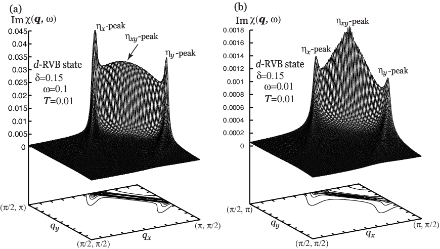
In Fig. 3(a), we show the $q$-dependence of ${\rm Im}\chi(\mbox{\boldmath$q$},\,\omega)$ at $\omega=0.1$ in the region $\frac{\pi}{2}\leq q_{x},q_{y}\leq\pi$ together with the projected contour-lines on the $q$-plane. The overall structure of ${\rm Im}\chi(\mbox{\boldmath$q$},\,\omega)$ is almost 2d-like even in the state with the q-1dFS($x$), except for the absence of the exact tetragonal symmetry, $(q_{x},\,q_{y})\rightarrow(\pm q_{y},\,\pm q_{x})$. There exist two different incommensurate (IC-) peaks at $(\pi-2\pi\eta_{x},\,\pi)$ and $(\pi,\,\pi-2\pi\eta_{y})$, which we call the $\eta_{x}$-peak and the $\eta_{y}$-peak, respectively. These peaks are connected with each other by a ‘wall’, as seen from the dense contour lines in Fig. 3(a). The center of the ‘wall’ located at $(\pi-2\pi\eta_{xy},\,\pi-2\pi\eta_{xy})$ forms a local maximum or a diagonal IC (DIC-) peak, which we call the $\eta_{xy}$-peak. With decreasing $\omega$, the $\eta_{x},\eta_{y}$-peaks are rapidly suppressed compared with the $\eta_{xy}$-peak, and the latter then becomes dominant as shown in Fig. 3(b).

These structures of ${\rm Im}\chi(\mbox{\boldmath$q$},\,\omega)$ can be understood in terms of fermiology as follows. In the present q-1dFS($x$), $`2k_{F}$’-scattering vectors are located on the gray lines in Fig. 4. Along this gray line ${\rm Im}\chi(\mbox{\boldmath$q$},\,\omega)$ shows the ‘wall’ structure, and the locations of the $\eta_{xy}$-peak are denoted by $`+$’ and those of the $\eta_{x},\eta_{y}$-peaks by the open symbols. Since the same open symbols are connected by the reciprocal lattice unit, Umklapp processes also contribute to the $\eta_{x},\eta_{y}$-peaks. We show in Fig. 4 the main scattering processes for each peak around $(\pi,\,\pi)$. (Umklapp processes are not shown.) Each scattering process originates from the $d$-wave gap node. In particular, the $\eta_{xy}$-peak results from the scattering between the $d$-wave gap nodes. This is why the $\eta_{xy}$-peak becomes dominant at lower $\omega$.

To see the $\omega$-dependence of ${\rm Im}\chi(\mbox{\boldmath$q$},\,\omega)$ more clearly, we perform the $q$-scan along three lines, each of which is across the $\eta_{x}$-peak, the $\eta_{y}$-peak or the $\eta_{xy}$-peak, respectively, and show the result in Fig. 5 for several choices of $\omega$ at $\delta=0.10$. With increasing $\omega$, the peak becomes broader and the $\eta_{x},\eta_{y}$-peaks develop more rapidly than that of the $\eta_{xy}$-peak. The location of each peak does not change appreciably up to $\omega\sim 0.2$ and shifts toward $(\pi,\,\pi)$ at larger $\omega$. This insensitivity to $\omega$ is weakened for lower $\delta$ and is limited to $\omega$$\stackrel{{\scriptstyle<}}{{\sim}}$$0.1$ at $\delta=0.05$.

In Fig. 6, we show the $\delta$-dependence of ${\rm Im}\chi(\mbox{\boldmath$q$},\,\omega)$ at $\omega=0.01$. Both the $\eta_{x},\eta_{y}$-peaks and the $\eta_{xy}$-peak remain sharp down to low $\delta$. The latter develops at lower $\delta$ relative to the former.

To study effects of the $d$-wave gap, we show in Fig. 7 ${\rm Im}\chi(\mbox{\boldmath$q$},\,\omega)$ in the u-RVB state at several values of $\omega$. As in the $d$-RVB state (Fig. 5), sharp peaks exist up to $\omega\sim 0.1$, although such $\omega$-range is reduced compared with the $d$-RVB state, and the peak width gets broader. Hence, for the existence of the $\eta_{x},\eta_{y}$-peaks and the $\eta_{xy}$-peak, the $d$-wave gap is not essential but the q-1dFS is. (In §3.5, we will see that for the 2dFS such sharp peaks are possible only in the $d$-RVB state.)

Figure 8 shows ${\rm Im}\chi(\mbox{\boldmath$q$},\,\omega)$ as a function of $\omega$; $q$ is fixed to the peak position, $\eta_{y}=0.135\;(0.130)$ or $\eta_{xy}=0.066\;(0.058)$, in the $d$-RVB (u-RVB) state for $\delta=0.22$. Both the $\eta_{y}$-peak and the $\eta_{xy}$-peak are suppressed by the $d$-wave gap, because the $d$-wave gap reduces the density of states responsible to the low energy scattering. For the $\eta_{y}$-peak in the $d$-RVB, a gap-like behavior appears at low $\omega$, and becomes clearer with decreasing both $T$ and $\Gamma$ as shown by the thin line ($T=10^{-3}$ and $\Gamma=10^{-4}$) in Fig. 8(a). This gap, which we call magnetic gapmagneticgap $\omega_{\rm mg}$, is approximately given by

where $q$ is the scattering vector, $(\pi,\,\pi-2\pi\eta_{y})$, and $\mbox{\boldmath$k$}_{\rm node}$ is a $d$-wave gap node position on the FS. Since the $\eta_{xy}$-peak in the $d$-RVB results mainly from the scattering between the $d$-wave gap nodes (Fig. 4), the value of $\mbox{\boldmath$k$}_{\rm node}$ is estimated to be $-\frac{1}{2}(\pi-2\pi\eta_{xy},\,\pi-2\pi\eta_{xy})$. Substituting the values of $\eta_{xy}$ and $\eta_{y}$ into eq. (14), we get $\omega_{\rm mg}(\mbox{\boldmath$q$})=0.057$, which is in good agreement with Fig. 8(a). (This good agreement has also been checked for other hole density.) In Fig. 9, we plot $\omega_{\rm mg}(\mbox{\boldmath$q$})$ as a function of $\delta$ together with the $d$-wave singlet order $\Delta_{0}$. Note the different $\delta$-dependence between $\omega_{\rm mg}(\mbox{\boldmath$q$})$ and $\Delta_{0}$. (In Appendix B, we give analytic formulae for estimating the values of $\eta_{xy}$ and $\eta_{y}$. The magnitude of the magnetic gap is then obtained from eq. (14) without any calculations of ${\rm Im}\chi(\mbox{\boldmath$q$},\,\omega)$.)

On the other hand, the magnetic gap is zero at the $\eta_{xy}$-peak. This does not, however, mean that effects of the $d$-wave gap are smaller compared with the $\eta_{y}$-peak. Using the result shown in Fig. 8, we show in Fig. 10 the ratio,

for both the $\eta_{y}$-peak and the $\eta_{xy}$-peak as a function of $\omega$. At $\omega\approx 0$, the $d$-wave gap suppresses the $\eta_{y}$-peak more strongly than the $\eta_{xy}$-peak. However, once $\omega$ exceeds $\omega_{\rm mg}$, the suppression of the $\eta_{xy}$-peak becomes more prominent than the $\eta_{y}$-peak.

Next, we investigate effects of the interlayer hopping, $t_{\perp}$, on the (single-layer) results presented so far. This introduces mixing between the two kinds of q-1d bands. Details of the formalism are given in Appendix A.

Reflecting the relative shift of Cu sites by $[\frac{1}{2},\frac{1}{2},\frac{1}{2}]$ (tetragonal notation) between the adjacent CuO₂ layers, the band dispersion along the $k_{z}$-direction is obtained as

We set the interlayer transfer integral to be $t_{\perp}=0.05t^{(1)}$ so that the band width of $\epsilon_{\mbox{\boldmath$k$}}$ is about 0.1 times that of $\xi_{\mbox{\boldmath$k$}}$pickett. (We neglect the interlayer magnetic interaction, whose order is $\sim 10^{-5}J$thio; peters; lyons.) In Fig. 11, we show the FS at $k_{z}=0$ and $\pi$ obtained by setting $\Delta_{\mbox{\boldmath$k$}}=0$ in eq. (25). The FS consists of the outer FS (solid line in Fig. 11) and the inner FS (gray line).

Taking $q_{z}=0$, we show in Figs. 12(a) and 12(b) the $q$-dependence of ${\rm Im}\chi(\mbox{\boldmath$q$},\,\omega)$ at $\omega=0.01$ for $\delta=0.10$ and $0.22$ (bold solid line) in the $d$-RVB state, comparing it with the (single-layer) result for the q-1dFS($x$) (thin dotted line). The IC-peaks at $(\pi-2\pi\eta_{{}_{\rm IC}},\,\pi)$ and $(\pi,\,\pi-2\pi\eta_{{}_{\rm IC}})$ remain sharp, and recover the fourfold symmetry around $(\pi,\,\pi)$. The peak position is almost the same as that of the (single-layer) $\eta_{x},\eta_{y}$-peaks, and the width becomes slightly broader. On the other hand, the DIC-peak at $(\pi-2\pi\eta_{{}_{\rm DIC}},\,\pi-2\pi\eta_{{}_{\rm DIC}})$ gets much broader compared with the (single-layer) $\eta_{xy}$-peak and is largely suppressed at high $\delta$ $($$\stackrel{{\scriptstyle>}}{{\sim}}$$0.22)$.

Figures 12(c) and 12(d) show the results in the u-RVB state. As in the $d$-RVB, IC-peaks are seen, but the line shape changes qualitatively. The IC-peak has a hump on the $(\pi,\,\pi)$ side at $\delta=0.10$. This hump originates from the (single-layer) $\eta_{x}$-peak for the q-1dFS($x$). Such structure develops into a double-peak structure at higher $\delta$. With further increasing $\delta$ $($$\stackrel{{\scriptstyle>}}{{\sim}}$$0.23)$, the double peaks merge into a single sharp peak because of the decrease of the band anisotropy, $\alpha\rightarrow 1$. As for the DIC-peak, the line shape is almost the same as that for the (single-layer) q-1dFS($x$). The peak height relative to the IC-peak is suppressed at higher $\delta$ as in the case of the $d$-RVB.

With increasing $\omega$, the IC-peak develops more rapidly than the DIC-peak, and become broader so that the fine structures such as the hump or the double-peak structure are smeared. These $\omega$-dependence share the common features to the (single-layer) results shown in Figs. 5 and 7.

In Fig. 13, we plot the $\delta$-dependence of $\eta_{{}_{\rm IC}}$ and $\eta_{{}_{\rm DIC}}$ at $\omega=0.01{\rm}$ in the $d$-RVB (a) and u-RVB (b) — the $\eta_{{}_{\rm DIC}}$ at high $\delta$ is not shown since the peak height of the DIC-peak is less than 50% of the IC-peak. (For the low doping region $\delta\leq 0.05$ in the u-RVB, we take $r=0.2$, instead of $r=0.35$, to avoid magnetic instability in eq. (13).) In both states, the values of $\eta_{{}_{\rm IC}}$ and $\eta_{{}_{\rm DIC}}$ increase smoothly as a function of $\delta$, except in the region $0.18$$\stackrel{{\scriptstyle<}}{{\sim}}$$\delta$$\stackrel{{\scriptstyle<}}{{\sim}}$$0.23$ in the u-RVB, where ${\rm Im}\chi(\mbox{\boldmath$q$},\,\omega)$ shows the double peaks. Their peak positions are plotted by filled circles with different size so that the smaller indicates the position of the lower peak. Since the relative height changes from the larger $\eta_{{}_{\rm IC}}$ to the smaller $\eta_{{}_{\rm IC}}$ in $0.19$$\stackrel{{\scriptstyle<}}{{\sim}}$$\delta$$\stackrel{{\scriptstyle<}}{{\sim}}$$0.21$ in Fig. 13(b), this may appear as a saturation behavior of $\eta_{{}_{\rm IC}}$ in $0.15$$\stackrel{{\scriptstyle<}}{{\sim}}$$\delta$$\stackrel{{\scriptstyle<}}{{\sim}}$$0.20$.

At higher $\omega$, the $\delta$-dependence of $\eta_{{}_{\rm IC}}$ and $\eta_{{}_{\rm DIC}}$ in the $d$-RVB is almost the same as that at $\omega=0.01$, since the positions of the (single-layer) $\eta_{x},\eta_{y},\eta_{xy}$-peaks do not change appreciably with $\omega$ as shown in Fig. 5. In the u-RVB state, however, the value of $\eta_{{}_{\rm IC}}$ gets smaller especially in low $\delta($$\stackrel{{\scriptstyle<}}{{\sim}}$$0.15)$ and possible saturation behavior in $0.15$$\stackrel{{\scriptstyle<}}{{\sim}}$$\delta$$\stackrel{{\scriptstyle<}}{{\sim}}$$0.20$ is smeared out. This qualitative difference from that at $\omega=0.01$ is due to the smearing of the hump and the double-peak structures of ${\rm Im}\chi(\mbox{\boldmath$q$},\,\omega)$. In contrast, the value of $\eta_{{}_{\rm DIC}}$ remains almost the same with increasing $\omega$, as seen in the (single-layer) result shown in Fig. 7.

So far we have seen magnetic excitation at low $T$ $(=0.01J)$. With increasing $T$, the following two effects may be expected. (i) The IC-peaks are thermally smeared out to form a C-peak. (ii) The q-1dFS is destabilized and is replaced by a ‘2dFS’. Here the possible ‘2dFS’ is the one obtained with the same band parameters as used in § 2.1, but $F_{x}=F_{y}$ is kept for each $\delta$. The resulting FS at $\delta=0.15$ is ‘electron-like’ centered at $(0,\,0)$ as shown in Fig. 14.

We thus calculate ${\rm Im}\chi(\mbox{\boldmath$q$},\,\omega)$ for several choices of $T$ for both the q-1dFS and the ‘2dFS’ in the u-RVB state. We include the interlayer hopping and set $\omega=0.1$ and $\delta=0.15$. Figure 15 shows that the IC-peak exists for both FSs in $T$$\stackrel{{\scriptstyle<}}{{\sim}}$$0.1$. At $T=0.2$, however, a broad C-peak is realized for the q-1dFS, and a weak IC-peak or an essentially flat topped commensurate (C-) peak for the ‘2dFS’.

As we discussed in the previous paperyamase1, the present q-1d picture of the FS is consistent with the ARPES data in LSCOino. Moreover, recent data in ARPESzhou2, the $k$-space distribution of low-energy spectral weight integrated down to 30meV below Fermi energy, has turned out to be consistent with our predicted FS shown in Fig. 11. We, however, note a different arguments from ours that the FS in LSCO will be the 2dFS shown in Fig. 16ino. (Note the difference in topology from the ‘2dFS’ shown in Fig. 14.) We thus investigate the difference in magnetic excitation between the q-1dFS and the 2dFS here.

We take the band parameters, $t^{(1)}/J=4,t^{(2)}/t^{(1)}=-1/6$, and $t^{(3)}/t^{(1)}=1/5$ and determine mean fields by minimizing the free energy in the same fashion as §2.1, but now with $F_{x}=F_{y}$. We then obtain 2dFS shown in Fig. 16.

Using this 2dFS, we show ${\rm Im}\chi(\mbox{\boldmath$q$},\,\omega)$ for several choices of $\omega$ in Figs. 17(a) and 17(b). In the $d$-RVB, both the sharp IC-peak and the sharp DIC-peak are realized. In the u-RVB, however, a broad C-peak becomes dominant and the remnants of the IC,DIC-peaks appear as weak substructures. This feature contrasts with the case of the q-1dFS where the sharp IC,DIC-peaks are realized even in the u-RVB. This difference may be understood by noting that the 2dFS allows the scattering vector $(\pi,\,\pi)$ from one point to the other on the FS while the q-1dFS does not. (When we introduce hybridization between the two kinds of the q-1d bands, the resulting FS (Fig. 11) allows such $(\pi,\,\pi)$ scattering vectors. However, these scatterings occur through the interlayer hopping and do not contribute appreciably to ${\rm Im}\chi(\mbox{\boldmath$q$},\,\omega)$ as seen from Figs. 12(c) and 12(d).)

Now we discuss a possible q-1d picture of the FS in LSCO systems from the viewpoint of magnetic excitation. We take the following four subjects: (i) IC-peak at high temperature, (ii) $\omega$-dependence and magnetic gap, (iii) incommensurability versus hole density, and (iv) IC-peak versus DIC-peak.

We have seen in §3.4 that for the 2dFS (Fig. 16) the IC-peak is realized only in the $d$-RVB state and is replaced by the essentially C-peak in the u-RVB state within the $\omega$-range studied here. This feature is consistent with experimental data for YBCOdai; arai; bourges. Moreover, the 2dFS shown in Fig. 16 is consistent with the FS observed by ARPESschabel. We therefore consider that magnetic excitation in YBCO systems may be understood on the basis of the 2dFS, as has been discussed theoreticallytanamoto2; lee; levin.

We have seen that fermiology can be a central concept for understanding magnetic excitation in high-$T_{\rm c}$ cuprates. This viewpoint contrasts with the ‘spin-charge stripes’ scenariotranquada1; tranquada2; tranquada3 where it is the formation of ‘charge stripes’, not effects of the FS, that gives rise to the magnetic IC,DIC-peaks.

Nonetheless, possible realization of the ‘charge stripes’ is interesting. In the present study, we have assumed that the charge density is uniform. When we relax this restriction, some kind of charge ordering may be stabilized in the state with a q-1dFS, which we are trying to clarify.

In §2.1, we have fit a q-1dFS near $(\pi,\,0)$ or $(0,\,\pi)$ to the observed FS segments by ARPESino. Figure 2 implies that band anisotropy remains even at high $\delta\,($$\stackrel{{\scriptstyle>}}{{\sim}}$$0.20)$. Such band anisotropy, however, can not be understood in terms of our previous argumentsyamase2 (see §1), since the crystal structure in LSCO with $\delta$$\stackrel{{\scriptstyle>}}{{\sim}}$$0.20$yamada is the HTT where we expect a ‘2dFS’. This problem should be resolved in a future.

References

- (1) J. M. Tranquada, B. J. Sternlieb, J. D. Axe, Y. Nakamura and S. Uchida: Nature 375 (1995) 561.
- (2) J. M. Tranquada, J. D. Axe, N. Ichikawa, Y. Nakamura, S. Uchida and B. Nachumi: Phys. Rev. B 54 (1996) 7489.
- (3) J. M. Tranquada, J. D. Axe, N. Ichikawa, A. R. Moodenbaugh, Y. Nakamura and S. Uchida: Phys. Rev. Lett. 78 (1997) 338.
- (4) N. Ichikawa, S. Uchida, J. M. Tranquada, T. Niemöller, P. M. Gehring, S.-H. Lee and J. R. Schneider: Phys. Rev. Lett. 85 (2000) 1738.
- (5) M. V. Zimmermann, A. Vigliante, T. Niemöller, N. Ichikawa, T. Frello, J. Madsen, P. Wochner, S. Uchida, N. H. Andersen, J. M. Tranquada, D. Gibbs and J. R. Schneider: Europhys. Lett. 41 (1998) 629.
- (6) T. Niemöller, N. Ichikawa, T. Frello, H. Hünnefeld, N. H. Andersen, S.Uchida, J. R. Schneider and J. M. Tranquada: Eur. Phys. J. B 12 (1999) 509.
- (7) More precisely, the superlattice peaks are observed only at , and the extinction at has been argued as due to structure factorstranquada2.
- (8) V. J. Emery, S. A. Kivelson and O. Zacher: Phys. Rev. B 56 (1997) 6120.
- (9) S. A. Kivelson, E. Fradokin and V. J. Emery: Nature 393 (1998) 550.
- (10) M. I. Salkola, V. J. Emery and S. A. Kivelson: Phys. Rev. Lett. 77 (1996) 155.
- (11) T. Tohyama, S. Nagai, Y. Shibata and S. Maekawa: Phys. Rev. Lett. 82 (1999) 4910.
- (12) K. Machida and M. Ichioka: J. Phys. Soc. Jpn. 68 (1999) 2168; M. Ichioka and K. Machida: ibid. 68 (1999) 4020.
- (13) H. Yamase and H. Kohno: J. Phys. Soc. Jpn. 69 (2000) 332; H. Yamase, H. Kohno and H. Fukuyama: Physica B 284–288 (2000) 1375.
- (14) H. Yamase and H. Kohno: J. Phys. Soc. Jpn. 69 (2000) 2151.
- (15) H. Yamase, H. Kohno and H. Fukuyama: Physica C 341–348 (2000) 321.
- (16) A. Ino, C. Kim, T. Mizokawa, Z.-X. Shen, A. Fujimori, M. Takaba, K. Tamasaku, H. Eisaki and S. Uchida: J. Phys. Soc. Jpn. 68 (1999) 1496; A. Ino, C. Kim, M. Nakamura, T. Yoshida, T. Mizokawa, Z.-X. Shen, A. Fujimori, T. Kakeshita, H. Eisaki and S. Uchida: cond-mat/0005370.
- (17) K. Yamada, C. H. Lee, K. Kurahashi, J. Wada, S. Wakimoto, S. Ueki, H. Kimura, Y. Endoh, S. Hosoya, G. Shirane, R. J. Birgeneau, M. Greven, M. A. Kastner and Y. J. Kim: Phys. Rev. B 57 (1998) 6165.
- (18) M. K. Crawford, R. L. Harlow, E. M. McCarron, W. E. Farneth, J. D. Axe, H. Chou and Q. Huang: Phys. Rev. B 44 (1991) 7749.
- (19) B. Büchner, M. Breuer, A. Freimuth and A. P. Kampf: Phys. Rev. Lett. 73 (1994) 1841.
- (20) S. Sakita, F. Nakamura, T. Suzuki and T. Fujita: J. Phys. Soc. Jpn. 68 (1999) 2755.
- (21) T. R. Thurston, R. J. Birgeneau, D. R. Gabbe, H. P. Jenssen, M. A. Kastner, P. J. Picone, N. W. Preyer, J. D. Axe, P. Böni, G. Shirane, M. Sato, K. Fukuda and S. Shamoto: Phys. Rev. B 39 (1989) 4327.
- (22) C. H. Lee, K. Yamada, M. Arai, S. Wakimoto, S. Hosoya and Y. Endoh: Physica C 257 (1996) 264.
- (23) H. Kimura, K. Hirota, C. H. Lee, K. Yamada and G. Shirane: J. Phys. Soc. Jpn. 69 (2000) 851.
- (24) C. J. Halboth and W. Metzner: Phys. Rev. Lett. 85 (2000) 5162.
- (25) T. Tanamoto, H. Kohno and H. Fukuyama: J. Phys. Soc. Jpn. 61 (1992) 1886; ibid. 62 (1993) 717.
- (26) We consider to be equal to the Sr2+ concentration, .
- (27) T. Tanamoto, H. Kohno and H. Fukuyama: J. Phys. Soc. Jpn. 62 (1993) 1455; ibid. 63 (1994) 2739.
- (28) The magnetic gap is often referred to the ‘spin gap’. In this paper, however, we use the ‘spin gap’ as a terminology indicating the normal state gap.
- (29) W. E. Pickett: Rev. Mod. Phys. 61 (1989) 433.
- (30) C. J. Peters, R. J. Birgeneau, M. A. Kastner, H. Yoshizawa, Y. Endoh, J. Tranquada, G. Shirane, Y. Hidaka, M. Oda, M. Suzuki and T. Murakami: Phys. Rev. B 37 (1988) 9761.
- (31) T. Thio, T. R. Thurston, N. W. Preyer, P. J. Picone, M. A. Kastner, H. P. Jenssen, D. R. Gabbe, C. Y. Chen, R. J. Birgeneau and A. Aharony: Phys. Rev. B 38 (1988) 905.
- (32) K. B. Lyons, P. A. Fleury, J. P. Remeika, A. C. Cooper and T. J. Negran: Phys. Rev. B 37 (1988) 2353.
- (33) X. J. Zhou, T. Yoshida, S. A. Kellar, P. V. Bogdanov, E. D. Lu, A. Lanzara, M. Nakamura, T. Noda, T. Kakeshita, H. Eisaki, S. Uchida, A. Fujimori, Z. Hussain and Z.-X. Shen: Phys. Rev. Lett. 86 (2001) 5578.
- (34) G. Aeppli, T. E. Mason, S. M. Hayden, H. A. Mook and J. Kulda: Science 278 (1997) 1432.
- (35) T. E. Mason, G. Aeppli and H. A. Mook: Phys. Rev. Lett. 68 (1992) 1414.
- (36) T. Nakano, N. Momono, M. Oda and M. Ido: J. Phys. Soc. Jpn. 67 (1998) 2622.
- (37) N. Momono, T. Matsuzaki, T. Nagata, M. Oda and M. Ido: J. Low Temp. Phys. 117 (1999) 353.
- (38) S. Ohsugi, Y. Kitaoka, K. Ishida, G. Zheng and K. Asayama: J. Phys. Soc. Jpn. 60 (1991) 2351; ibid. 63 (1994) 700.
- (39) M. Matsuda, K. Yamada, Y. Endoh, T. R. Thurston, G. Shirane, R. J. Birgeneau, M. A. Kastner, I. Tanaka and H. Kojima: Phys. Rev. B 49 (1994) 6958.
- (40) C. H. Lee, K. Yamada, Y. Endoh, G. Shirane, R. J. Birgeneau, M. A. Kastner, M. Greven and Y.-J. Kim: J. Phys. Soc. Jpn. 69 (2000) 1170.
- (41) B. Lake, G. Aeppli, T. E. Mason, A. Schröder, D. F. McMorrow, K. Lefmann, M. Isshiki, M. Nohara, H. Takagi and S. M. Hayden: Nature 400 (1999) 43.
- (42) H. Yamase, H. Kohno, H. Fukuyama and M. Ogata: J. Phys. Soc. Jpn. 68 (1999) 1082; J. Phys. Chem. Solids 60 (1999) 1063.
- (43) H. Matsushita, H. Kimura, M. Fujita, K. Yamada, K. Hirota and Y. Endoh: J. Phys. Chem. Solids. 60 (1999) 1071.
- (44) T. Suzuki, T. Goto, K. Chiba, T. Shinoda, T. Fukase, H. Kimura, K. Yamada, M. Ohashi and Y. Yamaguchi: Phys. Rev. B 57 (1998) R3229.
- (45) H. Kimura, K. Hirota, H. Matushita, K. Yamada, Y. Endoh, S. H. Lee, C. F. Majkrzak, R. Erwin, G. Shirane, M. Greven, Y. S. Lee, M. A. Kastner and R. J. Birgeneau: Phys. Rev. B 59 (1999) 6517.
- (46) K. Yamada: private communications.
- (47) N. Ichikawa: Doctor Thesis, University of Tokyo, Tokyo, 1999.
- (48) N. Ichikawa: private communications.
- (49) S. Wakimoto, R. J. Birgeneau, M. A. Kastner, Y. S. Lee, R. Erwin, P. M. Gehring, S. H. Lee, M. Fujita, K. Yamada, Y. Endoh, K. Hirota and G. Shirane: Phys. Rev. B 61 (2000) 3699.
- (50) M. Matsuda, M. Fujita, K. Yamada, R. J. Birgeneau, M. A. Kastner, H. Hiraka, Y. Endoh, S. Wakimoto and G. Shirane: Phys. Rev. B 62 (2000) 9148.
- (51) M. Fujita, K. Yamada, H. Hiraka, P. M. Gehring, S. H. Lee, S. Wakimoto and G. Shirane: cond-mat/010320.
- (52) H. Fukuyama: J. Phys. Chem. Solids 59 (1998) 447.
- (53) P. Dai, H. A. Mook and F. Dǒgan: Phys. Rev. Lett. 80 (1998) 1738.
- (54) M. Arai, T. Nishijima, Y. Endoh, T. Egami, S. Tajima, K. Tomimoto, Y. Shiohara, M. Takahashi, A. Garrett and S. M. Bennington: Phys. Rev. Lett. 83 (1999) 608.
- (55) P. Bourges, Y. Sidis, H. F. Fong, L. P. Regnault, J. Bossy, A. Ivanov and B. Keimer: Science 288 (2000) 1234.
- (56) M. C. Schabel, C.-H. Park, A. Matsuura, Z.-X. Shen, D. A. Bonn, Ruixing Liang and W. N. Hardy: Phys. Rev. B 57 (1998) 6107.
- (57) J. Brinckmann and P. A. Lee: Phys. Rev. Lett. 82 (1999) 2915.
- (58) Q. Si, Y. Zha, K. Levin and J. P. Lu: Phys. Rev. B 47 (1993) 9055; Y. Zha, K. Levin and Q. Si: ibid. 47 (1993) 9124; D. Z. Liu, Y. Zha and K. Levin: Phys. Rev. Lett. 75 (1995) 4130; Y.-J. Kao, Q. Si and K. Levin: Phys. Rev. B 61 (2000) R11898.