Optimal Bayesian Smoothing of Functional Observations over a Large Graph

Functional observations at various locations are commonly encountered in spatial statistics, and are often called spatio-temporal data. Extracting the underlying signal from such noisy spatio-temporal data involves smoothing over both space and time. In the Bayesian context, Gaussian processes are often used to describe spatio-temporal measurements (Banerjee et al. 2014). Functional data can also be associated with subjects, for instance, in medical or financial applications. In the modern era, the internet traffic data, or data obtained from wearable devices, are functional in nature, and are typically collected from many sources simultaneously. Unlike in the spatial context, a clear notion of the closeness of physical locations over which a smoothing can be carried out may be lacking, but some other notion of connectivity may be meaningful. Such a complex relational network may be described by a graph, with subjects standing for the nodes of the graph, and an edge connecting two nodes stands for a relation. Typically, the underlying graph has a large number of nodes. In most contexts, the graph is given or is easily identified. For instance, in spatial statistics, closeness of physical locations may clearly define neighboring nodes and constitute a graph, while in other contexts such as a protein interaction network (Sharan et al. 2007) or an image interpolation problem (Liu et al. 2013), the graph structure comes from the nature of the problem. In some other contexts such as voting patterns by politicians on issues (Poole and Rosenthal 1991), the graph may have to be estimated from the data using models for interaction such as the Ising model (Cipra 1987).

When the observations at the nodes of the graph are scalar measurements, an asymptotic framework for assessing the estimation of their parameters was proposed by Kirichenko and van Zanten 2018 in terms of the so-called graph-Laplacian. The growth of the eigenvalues of the graph-Laplacian leads to a notion of a dimension of the graph. Kirichenko and van Zanten 2018 introduced smoothness classes determined by a weighted Euclidean distance on the parameter vector using an appropriate power of the graph-Laplacian, depending on the dimension of the graph. Then they obtained the minimax rates of estimation in these smoothness classes under infill asymptotics. Kirichenko and van Zanten 2017 developed a Bayesian procedure using a multivariate normal prior with an appropriate dispersion matrix, and showed that the resulting Bayesian procedure achieves the minimax rate of estimation. Further, as the prior does not use the knowledge of smoothness, the obtained rate automatically adapts to the smoothness.

In this paper, we consider functional observations over a domain $\mathbb{T}$ at the nodes of a graph. The goal is to optimally recover their underlying mean functions. The functional observations are assumed to be distributed according to Gaussian processes on $\mathbb{L}_{2}(\mathbb{T})$, the space of square-integrable functions on $\mathbb{T}$. Multidimensional observations at nodes are treated by considering a finite set $\mathbb{T}$, while a continuous domain gives functional observations. We characterize the minimax rate for inference on the vector of means taking values in a certain type of smoothness classes in $(\mathbb{L}_{2}(\mathbb{T}))^{n}$. We then construct a Bayesian procedure using a joint Gaussian process prior with covariance kernel determined by an appropriate power of the graph-Laplacian when the smoothness level is given. We show that the posterior contraction rate equals the minimax rate, thus showing the asymptotic optimality of the proposed Bayesian procedure in the frequentist sense. We note that as the function becomes infinitely smooth, we recover the rate obtained by Kirichenko and van Zanten 2017 for scalar observations. As the graphical smoothness increases indefinitely, the classical setting with independent and identically distributed (i.i.d.) replications of functional observations is approached and standard rates for one-dimensional function smoothing are recovered. By using a random series prior with an unspecified number of terms, we show that the Bayesian procedure can adapt to the unknown smoothness, in that a single prior achieves the obtained rate simultaneously for all levels of smoothness, within a logarithmic factor. Then, we show that in a fixed smoothness setting, with an optimal choice of the prior, a posterior credible ball inflated by an appropriate constant, has frequentist coverage converging to one. Therefore, the resulting credible ball, which is easy to obtain by posterior simulation, can serve as a confidence ball in the frequentist sense, thus justifying Bayesian uncertainty quantification in the frequentist sense. The result is new even in the context of scalar observations. Finally, a posterior contraction result for discrete domain quantifying the accuracy of estimating trend of a multivariate time series is presented.

The following notations will be used throughout the paper. The symbols ‘$\lesssim$’ ‘$\gtrsim$’ will stand for inequality up to an unimportant constant multiple, and $\asymp$ for the equality of the order of magnitude. For a vector $a$ (respectively matrix $\mathrm{A}$), $a^{\tiny{\mathrm{T}}}$ (respectively, $\mathrm{A}^{\tiny{\mathrm{T}}}$) will denote the transpose. Let $\mathrm{I}$ stand for the $n\times n$ identity matrix. The indicator function is denoted by $\mathbbm{1}$ and the number of elements of a finite set by $\#$.

The paper is organized as follows. In the next section, we describe the model, present the preliminaries on graph-Laplacian and multidimensional Gaussian processes, and introduce the prior. In Section 3, the minimax rate is characterized, posterior contraction rates are obtained in both known and unknown smoothness settings, and asymptotic coverage of an appropriate credible ball is obtained. A simulation study comparing the performance of the proposed procedure with the random forest and a parallelly implemented univariate time series imputation algorithm is presented in Section 4. The proposed method is also illustrated with a daily temperature data at weather stations in North Carolina. Proofs are given in the appendix.

Let $G=(V,E)$ stand for a connected undirected graph with the set of nodes $V$, where $E\subset V\times V$ is the set of edges not containing any diagonal element. Suppose that with each node $i\in V$, there is an associated characteristic $f_{i}$, which is assumed to “change gradually over neighboring nodes”. The notion of a gradual change can be made precise when the cardinality $n$ of $V$ is large, in a manner similar to in-fill asymptotics used on a lattice. However, unlike the latter case where grid-points are regularly placed and the geometry is homogeneous, a notion of smoothness on a graph should take the structure of the graph in consideration. This can be captured by the adjacency matrix $\mathrm{A}=(\!(a_{ij})\!)$ with $a_{ij}=\mathbbm{1}\{(i,j)\in E\}$. Let $\mathrm{D}=(\!(d_{ij})\!)$ stand for the diagonal matrix with $d_{ii}=\#\{j\in V:(i,j)\in E\}$, the degree of the $i$th node. Then the graph-Laplacian is defined by $\mathrm{L}=\mathrm{D}-\mathrm{A}$. Clearly, $\mathrm{L}$ is symmetric, and can be shown to be positive semi-definite with the minimum eigenvalue always $0$ (corresponding to the eigenvector $(1,\ldots,1)$) and all other eigenvalues are positive. Let $0=\lambda_{0}<\lambda_{1}\leq\cdots\leq\lambda_{n-1}$ stand for the eigenvalues of $\mathrm{L}$. A common situation is that

for some constants $C_{1},C_{2}$, positive integer $i_{0}$, $\kappa\in(0,1]$, and $r\geq 1$, known as the dimension of the graph. For instance, if the graph is a $d$-dimensional lattice, $r=d$, so $r$ generalizes the notion of dimension to a general graph. By a result of Mohar et al. 1991, $\lambda_{1}\geq 4/n^{2}$, so $r<1$ is not possible. The value of $r$ may be obtained numerically by regressing $\log\lambda_{i}$ against $\log i$, such as in the small world-graph (Watts and Strogatz 1998) and a protein-interaction graph (Kolaczyk and Csárdi 2014), or for the dataset used in Section 4. As argued in Kirichenko and van Zanten 2017, we may assume that $\kappa=1$ in (2.1) at the expense of a larger value for the constant $C_{2}$.

When the characteristics associated with the nodes are real-valued, the object of interest is an $n$-dimensional column vector $f=(f_{1},\ldots,f_{n})^{\tiny{\mathrm{T}}}$, and the accuracy of estimation is measured by the normalized Euclidean norm $(n^{-1}\sum_{i=1}^{n}f_{i}^{2})^{1/2}$, Kirichenko and van Zanten 2017; Kirichenko and van Zanten 2018 considered smoothness classes based on the graph-Laplacian as follows: a Sobolev ball of regularity $\beta$ and radius $Q$ is defined to be $H^{\beta}(Q)=\{f:f^{\tiny{\mathrm{T}}}(\mathrm{I}+(n^{2/r}\mathrm{L})^{\beta})f\leq nQ^{2}\}$. The primary motivation behind the choice is that if the graph is a one-dimensional lattice (so $r=1$) and $f_{i}=f(i/n)$ for some smooth function $f$ on $[0,1]$, then the regularity $\beta=1$ in the above sense corresponds to the Sobolev regularity of order $1$ for the function $f$. Under this setting, Kirichenko and van Zanten 2018 showed that, based on independent observations $Y_{i}\sim\mathrm{N}(f_{i},\sigma^{2})$ where $\sigma$ is fixed or lies in a compact subinterval of $(0,\infty)$, the minimax rate of estimation in $H^{\beta}(Q)$ is $n^{-\beta/(2\beta+r)}$. This can be achieved by a multivariate normal prior on $f$:

provided that $\beta\leq\alpha+r/2$. The matrix powers are well-defined through the spectral theorem in view of the nonnegative definiteness of $\mathrm{L}$. Because the prior does not depend on the underlying regularity index $\beta$, the Bayesian method is automatically rate-adaptive, on the range $\beta\in(0,\alpha+r/2]$. They also showed that the full-range adaptation up to a logarithmic factor is possible using a different prior based on the exponential of the Laplacian.

To generalize the results of Kirichenko and van Zanten 2017; Kirichenko and van Zanten 2018 to functional observations, we model $Y_{1},\ldots,Y_{n}$ as independent Gaussian processes on $\mathbb{L}_{2}(\mathbb{T})$ for a compact domain $\mathbb{T}$, with mean functions $f_{1},\ldots,f_{n}$ respectively, and a common known covariance kernel $\sigma_{n}^{2}\Sigma$. The kernel $\Sigma$ acts as a compact operator on $\mathbb{L}_{2}(\mathbb{T})$, and hence has eigenvalues $\kappa_{j}\downarrow 0$. Let $\psi_{j}$ stand for the normalized eigenfunction of $\Sigma$ corresponding to the eigenvalue $\kappa_{j}$. Since Bayesian inference needs a likelihood function, the family of measures of $Y=(Y_{1},\ldots,Y_{n})^{\tiny{\mathrm{T}}}$ as $(f_{1},\ldots,f_{n})^{\tiny{\mathrm{T}}}$ varies over possible values must be absolutely continuous with respect to each other. This can hold only if $f_{1},\ldots,f_{n}$ belong to the reproducing kernel Hilbert space (RKHS) $\mathbb{H}$ of the covariance kernel $\Sigma$; see Appendix I of Ghosal and van der Vaart 2017. The RKHS $\mathbb{H}$ is a subspace of $\mathbb{L}_{2}(\mathbb{T})$ consisting of functions $g=\sum_{j=1}^{\infty}\kappa_{j}^{1/2}\theta_{j}\psi_{j}$, where $\sum_{j=1}^{\infty}\theta_{j}^{2}<\infty$. The RKHS norm $\|\cdot\|_{\mathbb{H}}$ on $\mathbb{H}$ given by $\|g\|_{\mathbb{H}}^{2}=\sum_{j=1}^{\infty}\theta_{j}^{2}$ makes $\mathbb{H}$ a Hilbert space.

The space where $f=(f_{1},\ldots,f_{n})^{\tiny{\mathrm{T}}}$ takes values is $\mathbb{H}^{n}$ equipped with the normalized aggregated norm $\|f\|_{n}=(n^{-1}\sum_{i=1}^{n}\|f_{i}\|_{\mathbb{H}}^{2})^{1/2}$. We denote the corresponding inner product by $\langle\cdot,\cdot\rangle_{n}$. Write $f_{i}=\sum_{j=1}^{\infty}\kappa_{j}^{1/2}\theta_{ij}\psi_{j}$, $i=1,2,\ldots$. Also let $\theta_{j}=(\theta_{1j},\ldots,\theta_{nj})^{\tiny{\mathrm{T}}}\in\mathbb{R}^{n}$ stand for the vector of the $j$th coefficients in the expansion of $f_{1},\ldots,f_{n}$ in terms of the basis $\mathcal{B}=(\psi_{1},\psi_{2},\ldots)$. Note that $f$ has an eigen-representation $f=\sum_{i=0}^{n-1}\sum_{j=1}^{\infty}\kappa_{j}^{1/2}\vartheta_{ij}\psi_{j}e_{i}$, where $e_{0},\ldots,e_{n-1}$ are the eigenvectors of $\mathrm{L}$ corresponding to the eigenvalues $\lambda_{0},\ldots,\lambda_{n-1}$. A equivalent canonical model is given by $Z_{ij}\sim\mathrm{N}(\vartheta_{ij},1)$ independently, where $Z_{ij}=\kappa_{j}^{-1/2}\int\langle Y,e_{i}\rangle\psi_{j}$ and $\vartheta_{ij}=\kappa_{j}^{-1/2}\int\langle f,e_{i}\rangle\psi_{j}$. Note that if $i\neq i^{\prime}$, $Z_{ij}$ and $Z_{i^{\prime}j^{\prime}}$ are clearly independent for any $j,j^{\prime}$, while $\mathrm{Cov}(Z_{ij},Z_{ij^{\prime}})=\kappa_{j}^{-1/2}\kappa_{j^{\prime}}^{-1/2}\int\!\int\Sigma(s,t)\psi_{j}(s)\psi_{j^{\prime}}(t)ds\,dt=(\kappa_{j}/\kappa_{j^{\prime}})^{1/2}\int\psi_{j}(t)\psi_{j^{\prime}}(t)dt=\mathbbm{1}(j=j^{\prime})$, so $Z_{ij}$ and $Z_{ij^{\prime}}$ are also independent for $j\neq j^{\prime}$.

The smoothness of a vector of functions on the graph can be described in terms of these coefficients. For $\beta,\gamma>0$, to quantify the regularity with respect to the graphical structure and the temporal direction respectively, define the $(\beta,\gamma)$-Sobolev ball $\mathcal{H}^{\beta,\gamma}(Q)$ of radius $Q$ in $\mathbb{H}^{n}$ by

To understand the notion, consider the white noise model $dY_{i}(t)=f_{i}(t)dt+dB_{i}(t)$ in the equivalent form $Y_{i}(t)=\int_{0}^{t}f_{i}(s)ds+B_{i}(t)$, where $B_{i}$ are independent standard Brownian motions. Then $\kappa_{2j-1}=\kappa_{2j}=j^{-1}$ and the smoothness $\gamma$ in the above sense coincides with the common Sobolev smoothness of each component function $f_{i}$.

We note that an $n\times n$-matrix $\mathrm{A}=(\!(a_{il})\!)$ can also be identified as a linear operator on $\mathbb{H}^{n}$ through the relation $\mathrm{A}(h_{1},\ldots,h_{n})^{\tiny{\mathrm{T}}}=(\sum_{l=1}^{n}a_{1l}h_{l},\ldots,\sum_{l=1}^{n}a_{nl}h_{l})^{\tiny{\mathrm{T}}}$ for any $(h_{1},\ldots,h_{n})^{\tiny{\mathrm{T}}}\in\mathbb{H}^{n}$. For an $n\times n$-matrix $\mathrm{A}$ and a linear operator $B$ on $\mathbb{H}$, define the Kronecker product $\mathrm{A}\otimes B$ to be a linear operator on $\mathbb{H}^{n}$ such that $(\mathrm{A}\otimes B)(h_{1},\ldots,h_{n})^{\tiny{\mathrm{T}}}=\mathrm{A}(Bh_{1},\ldots,Bh_{n})^{\tiny{\mathrm{T}}}$. If $\mathrm{A}$ is a (symmetric) nonnegative definite matrix and $B$ is a Hermitian nonnegative definite operator on $\mathbb{H}$, then it is easy to verify that $\mathrm{A}\otimes B$ is a Hermitian nonnegative definite operator on $\mathbb{H}^{n}$. If $\psi,\phi\in\mathbb{H}$, the tensor product $\psi\otimes\phi$ is a linear operator on $\mathbb{H}$ defined by $(\psi\otimes\phi)(h)=\langle\phi,h\rangle_{\mathbb{H}}\psi$.

We put a multivariate Gaussian process prior on $f\in\mathbb{H}^{n}$ with a separable covariance operator given by a tensor product $S(\mathrm{L})\otimes\Omega$, where $S(\mathrm{L})$ is a positive definite matrix depending on the graph Laplacian $\mathrm{L}$, and $\Omega$ is a covariance kernel on $\mathbb{H}$ with appropriate regularity. In the next section, we describe appropriate choices for $S(\mathrm{L})$ and $\Omega$.

We first obtain the minimax rate over Sobolev balls $\mathcal{H}^{\beta,\gamma}(Q)$ for any $Q>0$. The minimax risk for the problem is defined by $R_{n}=\inf_{T_{n}}\sup\{\mathrm{E}_{f}\|T_{n}-f\|_{2,n}^{2}:f\in\mathcal{H}^{\beta,\gamma}(Q)\}$, where the infimum is taken over all possible estimators. The decay rate of the square root of the minimax risk with $n$ is called the minimax rate.

To simplify certain bounds, we also make a simplifying assumption that $i_{0}=1$, and hence the smoothness condition given by the Sobolev ball can be simplified to $\sum_{i=1}^{n}\sum_{j=1}^{\infty}i^{2\beta/r}j^{2\gamma}\vartheta_{ij}^{2}\leq nQ^{2}$ after adjusting the constant $Q$. We assume throughout that $\sigma_{n}=1$, because the general case may be obtained by scaling: if $\epsilon_{n}$ is the rate obtained under this standard scaling, then the rate in the general case will be $\sigma_{n}\epsilon_{n}$.

To derive the minimax rate, we use the canonical form of the problem. Our proof will use the techniques of Tsybakov 2009 based on Pinsker’s theorem. This requires constructing the “Pinsker estimator” and studying its risk, which has been addressed so far only for a single sequence. Extension to the double-index setting is a major technical advancement.

It is natural to try and construct a Bayesian procedure attaining the minimax optimal rate. Recall that for a statistical model $\{X^{(n)}\sim P_{\theta}:\theta\in\Theta\}$ with prior $\theta\sim\Pi$, the posterior contraction rate at $\theta_{0}\in\Theta$ with respect to a metric $d$ is a sequence $\epsilon_{n}\to 0$ such that $P_{\theta_{0}}\Pi(\theta:d(\theta,\theta_{0})>M_{n}\epsilon_{n}|X^{(n)})\to 0$ for every $M_{n}\to\infty$. First we consider the case of known smoothness.

In our setting, we assume that the covariance kernel of the functional observations is completely known. By a slight extension of our arguments, we may include an unknown scale in the formulation as long as it remains bounded between two known positive numbers and is given a positive and continuous prior density on that interval. For simplicity, we forgo the more general statements; see Kirichenko and van Zanten 2017 for the additional arguments in the scalar case.

We note that if $\gamma\to\infty$, the underlying signal functionals become infinitely smooth, and the complexity of function estimation reduces to that of scalars or fixed dimensional objects. In this case, the posterior contraction rate coincides with $n^{-\beta/(2\beta+r)}$, the same rate Kirichenko and van Zanten 2017 obtained for real-valued observations on a graph. On the other hand, if $\beta\to\infty$, the problem reduces to that of replicated ordinary functional data and the posterior contraction rate coincides with the classical estimation rate $n^{-\gamma/(2\gamma+1)}$ for $\gamma$-smooth functions. It may be noted that we have used a more general Weibull prior on $c$ instead of the exponential used by Kirichenko and van Zanten 2017, to allow a broader range of values of $\gamma$ for larger $a$.

It is well-known that the posterior contraction rate is determined by the rate of concentration of the prior distribution near the true value in terms of the Kullback-Leibler divergence and the effective size of the parameter space measured by the metric entropy (Ghosal et al. 2000). For Gaussian process priors, van der Vaart and van Zanten 2008 further showed that these properties are controlled by the RKHS of the Gaussian process prior. Let the RKHS of $\mathrm{GP}(0,\Omega)$ with $\Omega$ in Theorem 2 be denoted by $\mathbb{K}\subset\mathbb{H}$ with RKHS norm $\|\cdot\|_{\mathbb{K}}$. It is easy to see that $\mathbb{K}=\{\sum_{j=1}^{\infty}\kappa_{j}^{1/2}z_{j}\psi_{j}:\sum_{j=1}^{\infty}j^{2\gamma+1}z_{j}^{2}<\infty\}$ with $\|\sum_{j=1}^{\infty}\kappa_{j}^{1/2}z_{j}\psi_{j}\|_{\mathbb{K}}^{2}=\sum_{j=1}^{\infty}j^{2\gamma+1}z_{j}^{2}$. Then for any fixed $c>0$, the RKHS of $\mathrm{GP}(0,(c/n)^{(2\alpha+r)/r}(\mathrm{L}+n^{-2}\mathrm{I})^{-(\alpha+r/2)}\otimes\Omega)$, and its approximation property and small ball probabilities are characterized in the following result. The primary challenge is to simultaneously address the variation over the graph and the time domain.

We note that the prior in Theorem 2 does not depend on the graphical smoothness $\beta$, and gives the targeted rate $n^{-\beta\gamma/(2\beta\gamma+\beta+r\gamma)}$, as long as $\beta\leq\alpha+r/2$. However, the prior needs to know the functional smoothness $\gamma$. The following result shows that a single prior can achieve this optimal rate (up to a logarithmic factor), that is, the Bayesian procedure adapts over the functional smoothness $\gamma$, as well as over the graphical smoothness $\beta$ on the whole range $(0,\infty)$. Here, we use a standard approach to adaptation over functional smoothness by considering a finite random series with a random number of terms (Shen and Ghosal 2015). To obtain adaptation over the graphical smoothness, unlike Kirichenko and van Zanten 2017 who used rescaled squared exponential Gaussian prior, we directly put a prior on the number of terms. The latter approach gives more numerical stability in the simulations.

A question of an immense interest is whether a Bayesian credible region obtained from the posterior distribution has adequate coverage. This is particularly relevant because providing a natural uncertainty quantification through the posterior distribution is an attractive feature of the Bayesian approach, and Bayesian credible sets are easy to obtain from posterior sampling. For fixed-dimensional regular families, the answer is affirmative in large samples. However, it was observed by Cox 1993, and further clarified by Knapik et al. 2011, that in a smooth signal estimation problem with a white noise, under the optimal smoothing, Bayesian credible sets can have arbitrarily low coverage probabilities. This is because under the optimal smoothing, the order of the bias matches that of the variability, thus shifting a credible region from its ideal position. The problem can be alleviated by controlling the bias to a manageable level. The approach pursued in Knapik et al. 2011 is undersmoothing, but this also makes the posterior contract sub-optimally. An alternative approach by inflating a credible region by a suitable constant (Szabó et al. 2015,Yoo and Ghosal 2016) will be pursued below. We assume that $i_{0}=1$ in (2.1) and the true smoothness $\beta$ and $\gamma$ are known and are not too low. We use a prior similar to Theorem 2 with a deterministic $c$ and choose the specific value $\alpha=\beta-r/2$.

The crux of the proof is to show that the posterior variation around its center is of the order of the variation of the posterior mean around the truth, and both matches the optimal rate. This will be done by a careful analysis of certain bias and variability terms of both the posterior distribution and the sampling distribution of the posterior mean. Explicit expressions obtained from conjugacy are very useful in this part, and hence the value of $c$ is deterministically chosen. The coverage also holds without the assumption $\gamma>\beta/r$, by only assuming that $\beta>r/2$, but then the diameter of the credible ball has a suboptimal order. The details are omitted, but the gap can be completed using some additional estimates obtained in the proof of the next theorem.

Now suppose that the functional data at the nodes are observed at regular grid points instead of continuously. More specifically, consider grid points $k/T$, $k=1,\ldots,T$, with meshwidth $T^{-1}$ and observations given by $Y_{i}(k/T)=f_{i}(k/T)+\varepsilon_{ik}$, where $f_{1},\ldots,f_{n}$ are the trend functions and $\varepsilon_{ik}$ are independent $\mathrm{N}(0,\sigma^{2})$ errors, $i=1,\ldots,n$, $k=1,\ldots,T$. These independent “nuggets” are thus random errors allowing fluctuations from a smooth trend of unknown functional form qualitatively related across neighboring nodes. The following result shows the posterior contraction rate for estimating the multivariate trend with respect to the normalized Euclidean distance $d_{n}(f,f^{*})=\big\{(nT)^{-1}\sum_{i=1}^{n}\sum_{k=1}^{T}|f_{i}(k/T)-f_{i}^{*}(k/T)|^{2}\big\}^{1/2}$ on the vector of trends, where $T=T_{n}$ gets larger with $n$. In this case, as the errors in the functional direction are also independent, a local smoothing in that direction also allows borrowing of information and $T$ plays an essential role in the rate. We put a prior on the signal functions through a discrete wavelet transformation of the whole collection of functions $(f_{1},\ldots,f_{n})$ and independent normal priors on the wavelet coefficients. After recovering the values of a function at the grid locations $k/T$, $k=1,\ldots,T$, we join the values by line-segments to construct the whole function. To simplify expressions in the proof, as in Theorem 5, we assume that $i_{0}=1$, so that $\lambda_{i}\asymp(i/n)^{2/r}$ for all $i=1,\ldots,n$. The functions are assumed to satisfy a discrete version of the graph-functional joint smoothness condition. We observe an interesting phase-transition phenomenon involving the relative values of the graphical and functional smoothness — if the individual functions are not sufficiently smooth compared with the smoothness in the graphical direction, the full benefit of the graphical smoothness may not be usable.

The theorem clearly shows the benefit of borrowing information across neighboring nodes: if each function is individually estimated, the accuracy of estimating the trend would have been only $T^{-\gamma/(2\gamma+1)}$. This assertion is numerically supported in our simulation results and the real-data analysis by the substantially lower prediction errors for our proposed methods compared with standard prediction techniques not taking the graphical relation in consideration.

In this section, we first study the performance of the proposed method on a set of simulated data, and later apply the method to analyze daily temperatures at several weather stations. We consider three different graphs. We consider a sparse weighted adjacency matrix that satisfies the geometry condition approximately. To obtain a weighted adjacency matrix with 100 nodes, we generate a $50\times 50$ symmetric matrix with entries uniformly generated from $(0,1)$ and delete the edges with a weight less than $0.8$. Furthermore, we generate two more graphs with 50 nodes, the Erdos-Reýni random graph using R package igraph (Csardi and Nepusz 2006) and cluster-type random graph using R package BDgraph (Mohammadi and Wit 2019). These graphs also approximately satisfy the geometry condition for different values of $r$ which is pre-computed following Kirichenko and van Zanten 2017. We consider 16 equidistant timepoints in the interval $[0,1]$. Our model is thus in discreet domain having the same setup as in Theorem 6. The true means is given by $f(t)=\sum_{i=0}^{n-1}3\sin\left(\frac{i}{2T}\right)\sqrt{n}i^{-1/2-2/r}e_{i}$, where $e_{i}$’s are the eigenvectors of the associated graph. The mean function then satisfies the smoothness condition with $\beta=2$. Subsequently, the data is generated as $Y_{i}(t)\sim\mathrm{N}(f_{i}(t),1)$. We generate 50 replicated datasets for each case.

Computational algorithm: We fit the model with prior : $\sigma^{-2}\sim$ Gamma$(0.1,0.1)$. Rest of the priors are as in Theorem 2. We implement an efficient Markov chain Monte Carlo (MCMC) sampling scheme for posterior computation. As described in Theorem6, our working model $f_{i}(k/T)$ is $f_{i}(k/T)=\sum_{m=1}^{n}\sum_{j=1}^{T}\vartheta_{mj}e_{mi}\psi_{j}(k/T)$. The error variance $\sigma^{2}$, and the coefficients $\vartheta_{mj}$’s are sampled using a Gibbs sampler from the full conditional conjugate posterior. To update the scale parameter $c$, we implement a Hamiltonian Monte Carlo (HMC) sampler (Neal 2011). To select optimal $\alpha$, we consider the 5-fold cross-validation framework. To implement our method, we generate 5000 post-burn MCMC samples after burn-in 5000 samples.

We discard 50% of data at random and train model in rest of the available data. Based on the estimated function from available data, we compute the mean at the missing locations and evaluate mean prediction MSE. In Table 1, we compare with the predicted values obtained by random forest using the R package missForest (Stekhoven and Bühlmann 2012), fPCA (functional PCA) method of fdapace (Carroll et al. 2021) and by univariate imputation technique using the R package imputeTS (Moritz and Bartz-Beielstein 2017). The former fits a random forest on the observed part and then predicts the missing part. It reports an out-of-bag imputation error using bootstrap aggregation. The imputeTS algorithm imputes using a spline based interpolation technique for each node independently. We use another method that uses singular value decomposition based missMDA (Josse and Husson 2016). Most standard imputation packages failed to produce any result. Examples include bootstrap based Amelia (Honaker et al. 2011), Expectation-Maximization (EM) algorithm based mtsdi (Junger and de Leon 2018), which are specially designed for spatio-temporal datasets and another EM based algorithm imputeR. In the simulation and data application, we consider wavelet bases to construct the prior variance $\Omega$. We also compute empirical coverages of the proposed method based on equal tail 95% credible intervals for the MCMC samples. Table 2 contrasts empirical coverages with the coverages due to inflated credible intervals. We set the inflation factor to $0.8\log n$ following Das and Ghosal 2017. Figure 1 compares the box plots across different methods based on the 50 simulated datasets. Spline estimates are omitted in this comparison due to their large magnitudes.

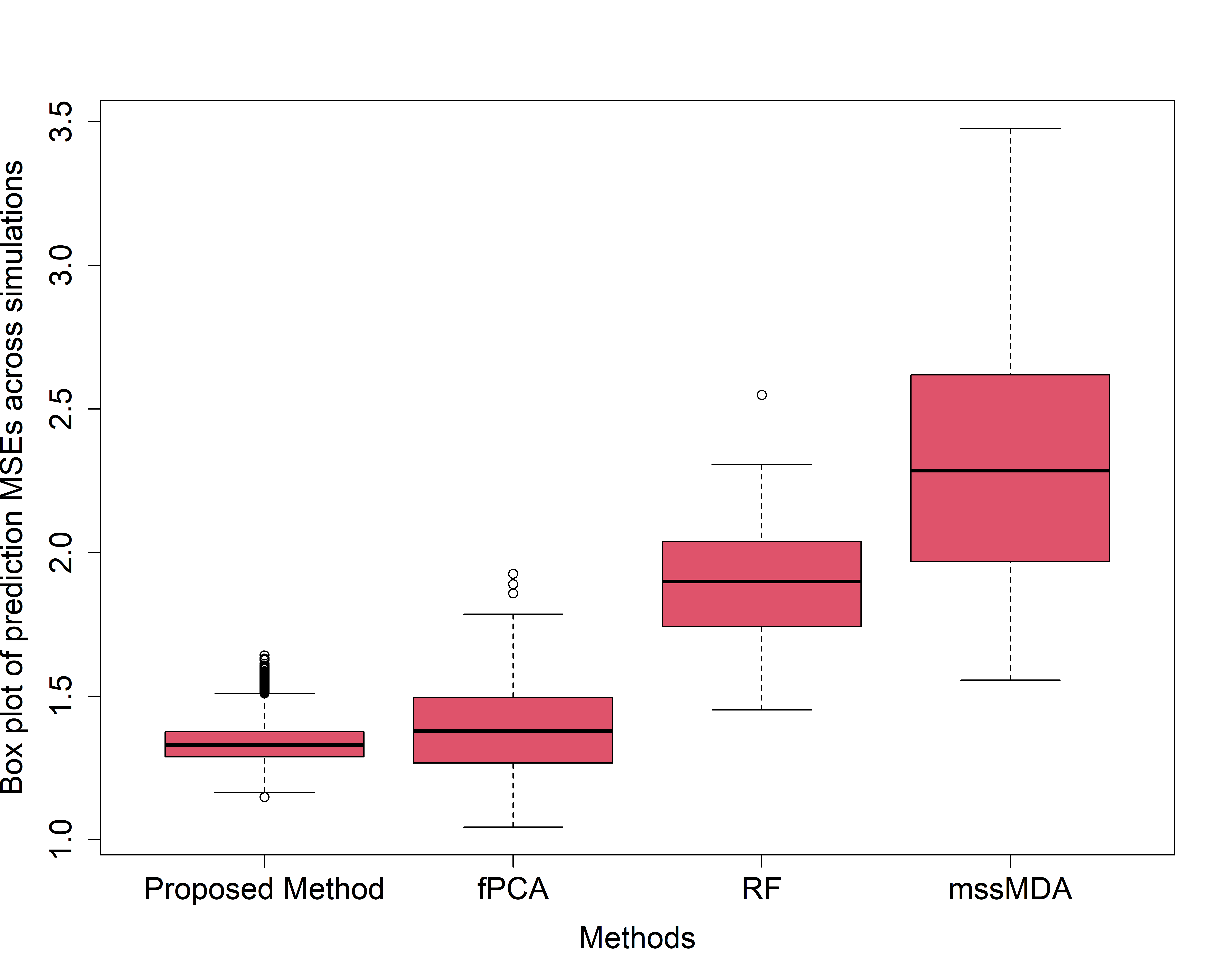
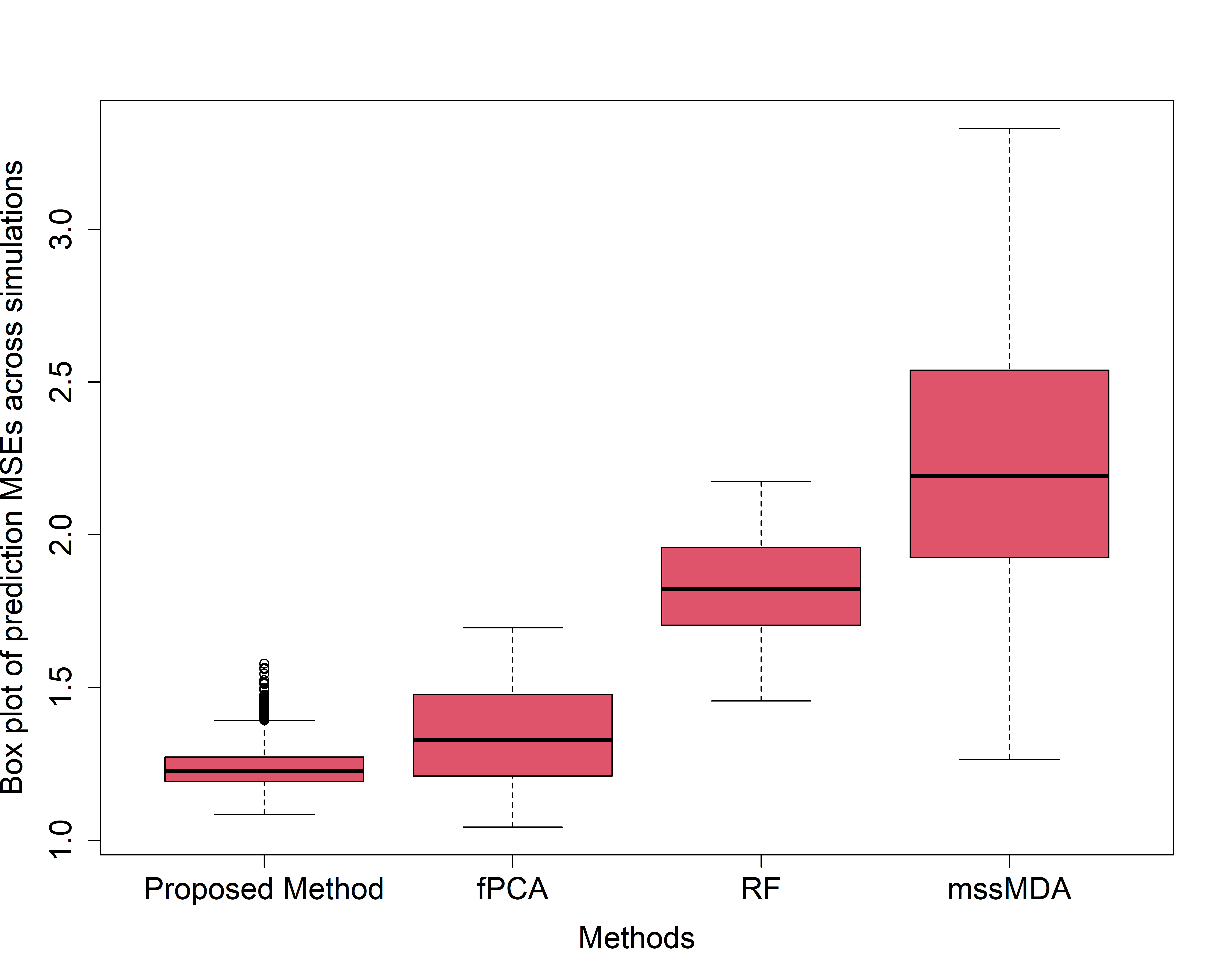
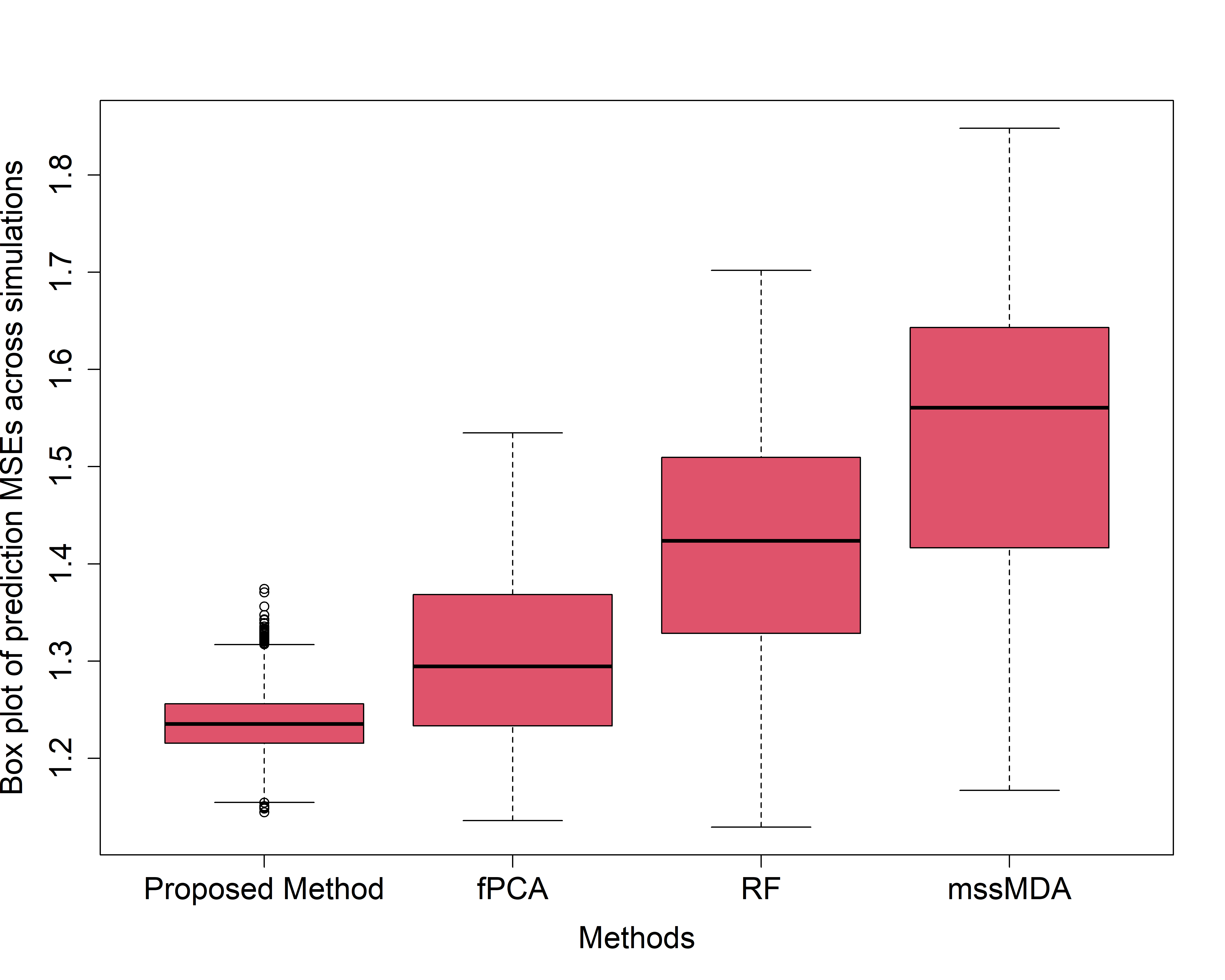
Now we illustrate the proposed method on a daily temperature dataset, collected by different weather stations across the US state of North Carolina. The dataset is downloaded from the website of the National Oceanic and Atmospheric Administration (NOAA). The values of daily average temperatures were collected at 158 weather locations over the year 2010. The dataset also contain the latitudes and longitudes of the weather stations. We construct weighted adjacency matrix ($A$) based on distances, as $A_{i,j}=10/d_{i,j}$. Here $d_{i,j}$ stands for the distance between $i$-$th$ and $j$-$th$ weather stations. In addition, we delete the edges having large $d_{i,j}$ to ensure sparsity. It is prudent to assume that the temperature reading of location (a) will have negligible impact on location (b) if there are geographically far apart. In this paper, we choose $70$-$th$ percentile of $d_{i,j}$’s as threshold. Thus, the resulting distanced based adjacency matrix in our case have $30\%$ non-zero weights after discarding the edges with large $d_{i,j}$. While studying evolution of mumps in England, Knight et al. 2016 also built a network structure among county towns based following a similar strategy. Figure 2 shows that the constructed binary adjacency matrix satisfies the geometry condition with dimension value $r=1.96$. We again randomly set aside $50\%$ of the observations for test data and train the model in rest. Based on the estimates, we predict at the missing locations and time points. Furthermore, we repeat this experiment using the data on four different months of the year. These four months are from four different seasons. We first mean-center and normalize the data. The comparisons here are limited to fPCA and PCA using missMDA. Other two competing methods from the simulation section could not provide estimates.

The statistical methods to analyze functional data have observed many new developments in the recent past (see Dabo-Niang and Ferraty 2008; Ferraty 2011; Goia and Vieu 2016; Aneiros et al. 2017; Aneiros et al. 2019). Functional PCA based approaches have been incredibly successful to model functional datasets in dense grid Hall et al. 2006. In Bayesian framework, clustering based approaches are proposed for functional clustering (Petrone et al. 2009; Rodríguez et al. 2009), and also in image regression (Meyer et al. 2015; Goldsmith et al. 2014). Wang et al. 2016 provides a thorough review on recent advancements on analyzing functional data.

In this work, we develop a method to study functional data on a given network. To the best of our knowledge, this is the first attempt on a network-linked FDA. The main novelties, apart from considering an FDA setup, is that we address the two-way smoothness issue, for studying minimax rate and Bayesian adaptation, a pioneering study, and we establish coverage in the graphical setting, which has not been done earlier even for scalar observations. There are some immediate extensions, we may consider. One extension could be modeling a multivariate functional dataset taking a two-stage approach. The graphical dependence may be computed in the first stage. The subsequent stage may apply our proposed functional data model using the estimated network from the first stage. Another extension may be to consider modeling time-varying networks.

We would like to thank the Editors of the journal, the editors of special issue, and reviewers for their constructive comments that improved presentation of the paper. The second author is partially funded by the ARO grant 76643-MA.

References

- Aneiros et al. (2017) Germán Aneiros, Enea G Bongiorno, Ricardo Cao, and Philippe Vieu. Functional statistics and related fields. Springer, 2017.
- Aneiros et al. (2019) Germán Aneiros, Ricardo Cao, and Philippe Vieu. Editorial on the special issue on functional data analysis and related topics, 2019.
- Banerjee et al. (2014) Sudipto Banerjee, Bradley P Carlin, and Alan E Gelfand. Hierarchical Modeling and Analysis for Spatial Data. CRC press, 2014.
- Belitser and Ghosal (2003) Eduard Belitser and Subhashis Ghosal. Adaptive Bayesian inference on the mean of an infinite-dimensional normal distribution. The Annals of Statistics, 31(2):536–559, 2003.
- Carroll et al. (2021) Cody Carroll, Alvaro Gajardo, Yaqing Chen, Xiongtao Dai, Jianing Fan, Pantelis Z. Hadjipantelis, Kyunghee Han, Hao Ji, Hans-Georg Mueller, and Jane-Ling Wang. fdapace: Functional Data Analysis and Empirical Dynamics, 2021. URL https://CRAN.R-project.org/package=fdapace. R package version 0.5.6.
- Cipra (1987) Barry A Cipra. An introduction to the Ising model. The American Mathematical Monthly, 94(10):937–959, 1987.
- Cox (1993) Dennis D Cox. An analysis of Bayesian inference for nonparametric regression. The Annals of Statistics, 21(2):903–923, 1993.
- Csardi and Nepusz (2006) Gabor Csardi and Tamas Nepusz. The igraph software package for complex network research. InterJournal, Complex Systems:1695, 2006. URL https://igraph.org.
- Dabo-Niang and Ferraty (2008) Sophie Dabo-Niang and Frédéric Ferraty. Functional and operatorial statistics. Springer Science & Business Media, 2008.
- Das and Ghosal (2017) Priyam Das and Subhashis Ghosal. Bayesian quantile regression using random b-spline series prior. Computational Statistics & Data Analysis, 109:121–143, 2017.
- Dunker et al. (1998) Th Dunker, MA Lifshits, and W Linde. Small deviation probabilities of sums of independent random variables. In High dimensional probability, pages 59–74. Springer, 1998.
- Ferraty (2011) Frédéric Ferraty. Recent advances in functional data analysis and related topics. 2011.
- Ghosal and van der Vaart (2017) Subhashis Ghosal and Aad van der Vaart. Fundamentals of Nonparametric Bayesian Inference. Cambridge University Press, Cambridge, 2017.
- Ghosal et al. (2000) Subhashis Ghosal, Jayanta K Ghosh, and Aad W van der Vaart. Convergence rates of posterior distributions. The Annals of Statistics, 28(2):500–531, 2000.
- Goia and Vieu (2016) A Goia and P Vieu. Special issue on statistical models and methods for high or infinite dimensional spaces. Journal of Multivariate Analysis, 146:1–352, 2016.
- Goldsmith et al. (2014) Jeff Goldsmith, Lei Huang, and Ciprian M Crainiceanu. Smooth scalar-on-image regression via spatial bayesian variable selection. Journal of Computational and Graphical Statistics, 23(1):46–64, 2014.
- Hall et al. (2006) Peter Hall, Hans-Georg Müller, and Jane-Ling Wang. Properties of principal component methods for functional and longitudinal data analysis. The annals of statistics, pages 1493–1517, 2006.
- Honaker et al. (2011) James Honaker, Gary King, and Matthew Blackwell. Amelia II: A program for missing data. Journal of Statistical Software, 45(7):1–47, 2011. URL http://www.jstatsoft.org/v45/i07/.
- Josse and Husson (2016) Julie Josse and François Husson. missMDA: A package for handling missing values in multivariate data analysis. Journal of Statistical Software, 70(1):1–31, 2016. doi: 10.18637/jss.v070.i01.
- Junger and de Leon (2018) Washington Junger and Antonio Ponce de Leon. mtsdi: Multivariate Time Series Data Imputation, 2018. URL https://CRAN.R-project.org/package=mtsdi. R package version 0.3.5.
- Kirichenko and van Zanten (2017) Alisa Kirichenko and Harry van Zanten. Estimating a smooth function on a large graph by Bayesian Laplacian regularisation. Electronic Journal of Statistics, 11(1):891–915, 2017.
- Kirichenko and van Zanten (2018) Alisa Kirichenko and Harry van Zanten. Minimax lower bounds for function estimation on graphs. Electronic Journal of Statistics, 12(1):651–666, 2018.
- Knapik et al. (2011) Bartek T Knapik, Aad W van der Vaart, and J Harry van Zanten. Bayesian inverse problems with Gaussian priors. The Annals of Statistics, 39(5):2626–2657, 2011.
- Knight et al. (2016) MI Knight, MA Nunes, and GP Nason. Modelling, detrending and decorrelation of network time series. arXiv preprint arXiv:1603.03221, 2016.
- Kolaczyk and Csárdi (2014) Eric D Kolaczyk and Gábor Csárdi. Statistical Analysis of Network Data with R, volume 65. Springer, 2014.
- Liu et al. (2013) Xianming Liu, Debin Zhao, Jiantao Zhou, Wen Gao, and Huifang Sun. Image interpolation via graph-based Bayesian label propagation. IEEE Transactions on Image Processing, 23(3):1084–1096, 2013.
- Meyer et al. (2015) Mark J Meyer, Brent A Coull, Francesco Versace, Paul Cinciripini, and Jeffrey S Morris. Bayesian function-on-function regression for multilevel functional data. Biometrics, 71(3):563–574, 2015.
- Mohammadi and Wit (2019) Reza Mohammadi and Ernst C. Wit. BDgraph: An R package for Bayesian structure learning in graphical models. Journal of Statistical Software, 89(3):1–30, 2019. doi: 10.18637/jss.v089.i03.
- Mohar et al. (1991) Bojan Mohar, Y Alavi, G Chartrand, and OR Oellermann. The Laplacian spectrum of graphs. Graph Theory, Combinatorics, and Applications, 2(12):871–898, 1991.
- Moritz and Bartz-Beielstein (2017) Steffen Moritz and Thomas Bartz-Beielstein. imputets: time series missing value imputation in r. R J., 9(1):207, 2017.
- Neal (2011) Radford M Neal. Mcmc using hamiltonian dynamics. Handbook of Markov Chain Monte Carlo, 2(11):2, 2011.
- Petrone et al. (2009) Sonia Petrone, Michele Guindani, and Alan E Gelfand. Hybrid dirichlet mixture models for functional data. Journal of the Royal Statistical Society: Series B (Statistical Methodology), 71(4):755–782, 2009.
- Poole and Rosenthal (1991) Keith T Poole and Howard Rosenthal. Patterns of congressional voting. American Journal of Political Science, 35(1):228–278, 1991.
- Rodríguez et al. (2009) Abel Rodríguez, David B Dunson, and Alan E Gelfand. Bayesian nonparametric functional data analysis through density estimation. Biometrika, 96(1):149–162, 2009.
- Sharan et al. (2007) Roded Sharan, Igor Ulitsky, and Ron Shamir. Network-based prediction of protein function. Molecular Systems Biology, 3(1), 2007.
- Shen and Ghosal (2015) Weining Shen and Subhashis Ghosal. Adaptive Bayesian procedures using random series priors. Scandinavian Journal of Statistics, 42(4):1194–1213, 2015.
- Stekhoven and Bühlmann (2012) Daniel J Stekhoven and Peter Bühlmann. Missforest—non-parametric missing value imputation for mixed-type data. Bioinformatics, 28(1):112–118, 2012.
- Szabó et al. (2015) Botond Szabó, Aad W Van Der Vaart, and JH van Zanten. Frequentist coverage of adaptive nonparametric Bayesian credible sets. The Annals of Statistics, 43(4):1391–1428, 2015.
- Tsybakov (2009) Alexandre B. Tsybakov. Introduction to Nonparametric Estimation. Springer Series in Statistics. Springer, New York., 2009.
- van der Vaart and van Zanten (2008) Aad W van der Vaart and J Harry van Zanten. Rates of contraction of posterior distributions based on Gaussian process priors. The Annals of Statistics, 36(3):1435–1463, 2008.
- Wang et al. (2016) Jane-Ling Wang, Jeng-Min Chiou, and Hans-Georg Müller. Functional data analysis. Annual Review of Statistics and Its Application, 3:257–295, 2016.
- Watts and Strogatz (1998) Duncan J Watts and Steven H Strogatz. Collective dynamics of ‘small-world’networks. Nature, 393(6684):440, 1998.
- Yoo and Ghosal (2016) William Weimin Yoo and Subhashis Ghosal. Supremum norm posterior contraction and credible sets for nonparametric multivariate regression. The Annals of Statistics, 44(3):1069–1102, 2016.