Portfolio Selection under Multivariate Merton Model with Correlated Jump Risk
Abstract.
Portfolio selection in the periodic investment of securities modeled by a multivariate Merton model with dependent jumps is considered. The optimization framework is designed to maximize expected terminal wealth when portfolio risk is measured by the Condition-Value-at-Risk (). Solving the portfolio optimization problem by Monte Carlo simulation often requires intensive and time-consuming computation; hence a faster and more efficient portfolio optimization method based on closed-form comonotonic bounds for the risk measure of the terminal wealth is proposed.
Keywords: Investment analysis, Conditional tail expectation, Merton model, Geometric Brownian motion, Comonotonicity.
2010 Mathematics Subject Classification: Primary C630; Secondary C580; C650
1. Introduction
The idea of portfolio optimization has been the focus of research groups and management teams since it was introduced by Markowitz in 1952 [13] and a wide variety of optimization methods using different financial models have been proposed. Dhaene et al. [7] studied multi-period portfolio selection in a Black-Scholes market. Kaas et al. [9] addressed the portfolio optimization problem with a constant mix strategy using comonotonic approximations and Weert et al. [20] extended their results to the selection of a multi-period portfolio related to a specific provisioning problem. Brown et al. [2] considered dynamic portfolio optimization in a discrete-time finite-horizon setting, and Xu et al. [21] studied portfolio optimization for a Black-Scholes market with stochastic drift. Recently Wang et al. [18] implemented the Merton model to price a power exchange option.
In this paper, we follow [18] and consider a multivariate Merton model with two kinds of dependent jumps. Uncommon jumps are such that the jump times in the marginal processes may differ from each other. These are individual jumps and occur upon the arrival of important new information which, for example, may have a marginal effect on the price only of certain stocks or cause an imbalance between their supply and demand thus changing their prices. Common jumps occur simultaneously in the marginal processes but the jump values may vary. These simultaneous jumps can be caused by changes in the investment rate, alterations in the economic outlook or other reasons that impose a price jump at a specific time on all stock values.
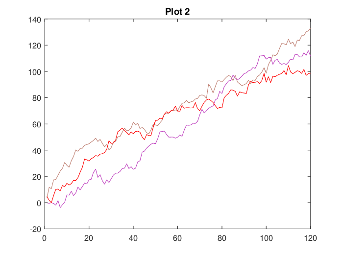
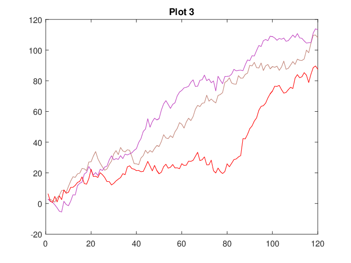
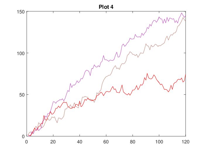
The flexibility of the Merton model enables it to fit financial data with correlated jumps and can be used to optimize a portfolio for a periodic investment problem in a constant mix strategy framework. Figure 1 illustrates this flexibility and compares it with three other models using simulated processes. The figure presents simulated data from four models, including processes without any jump terms (Plot 1), processes with common jumps but with different jump values (Plot 2), processes without common jumps (Plot 3), and processes with both types of jumps (Plot 4). These plots show the ability of the Merton model to take into account both individual jumps as well as jumps occurring at a specific times.

In order to solve the optimization problem for this model we need to solve a stochastic differential equation (SDE) corresponding to a portfolio containing multiple assets. In what follows we provide a closed-form solution for the terminal wealth process of the SDE corresponding to a constant mix strategy investment problem. To optimize a portfolio we maximize the terminal wealth process by controlling its risk measure and rather than applying numerical methods such as Monte Carlo Markov Chain (MCMC) to solve this optimization problem, we propose an alternative method using comonotonic bounds. This approach reduces computational complexity and returns a closed-form solution to the portfolio optimization problem for maximizing the expectation of terminal wealth when the corresponding risk measure of the comonotonic bound is under control.
The concept of comonotonicity has been thoroughly studied in actuarial and financial literature (Dhaene et al. [5] and Dhaene et al. [6]) and the assumption of comonotonic dependence structures between asset prices has proved to be a useful when solving financial problems such as derivative pricing (Deelstra et al. [3, 4] and Linders et al. [11]). Vanduffel et al. [17] used comonotonic approximations to obtain closed forms for the lower and upper bounds for the price of a continuously sampled European-style Asian option with fixed exercise price.
The rest of the paper is organized as follows. In Section 1 we introduce the Merton model, and review existing definitions and preliminary results. In Section 2, we present the main results; we first solve the SDE corresponding to the terminal wealth process of a portfolio following a jump-diffusion model containing one risk-free asset and risky assets and then obtain comonotonic bounds for the terminal wealth in order to solve the portfolio optimization problem while controlling of the terminal wealth. Proofs of all the results stated in this section may be found in the appendix. In Section 3, we carry out our optimization method on simulated data and data containing the daily prices of the stocks of Zoom Video Communication Inc. (ZM), and Tesla Inc. (TSLA) obtained from the market index.
Preliminaries
The base asset price in a Black-Scholes model follows the geometric Brownian motion process and the dynamics of the stock price are described by a continuous-time diffusion process whose sample path is continuous with probability one. Merton [14] illustrated that in order to satisfy the conditions of the Black-Scholes model, trading should take place continuously in time and the price dynamics of the stock should have a continuous sample path with probability one. However, since real world datasets are discrete realizations of variables and a continues path model does not provide for jumps, it is generally not suitable for real stock prices.
Following [18], we shall assume that all continuous time processes are Wiener and jump components are Poisson driven. Merton’s jump-diffusion model [15] is commonly used in literature and has abundant applications in financial data analysis. For example, Kolmanovsky et al. [10] applied this model to address the optimal containment control problem in a financial market, Wang et al. [19] investigated a power exchange option pricing problem assuming a jump-diffusion model, and Xu et al. [22] provided an analytical valuation of power exchange options based on the Merton model with dependent jumps. The model can be written as
where is the instantaneous expected return on the stock, is the instantaneous variance of the return conditional on arrival of no important new information, is a stochastic differential of the standard Brownian motion, and is a stochastic differential of a Poisson process defined based on the natural filtration of the random processes and . Moreover, and are assumed to be independent.
Bayraktar et al. [1] illustrated the advantages of the Merton model over a piecewise Markov model and Giesecke et al. [8] used it to study asset, commodity and energy prices, interest and exchange rates, and the timing of corporate and sovereign defaults.
In this paper, we study the return of a portfolio consisting of one risk-free asset together with several risky assets which follow the jump-diffusion Merton model. To be more specific, we assume that the jump risk common to all assets is diversifiable in the market and has a zero risk premium. This assumption ensures that there exists a risk neutral measure under which (for ), the dynamics of risky assets prices become
| (1.1) | |||||
where is the drift of geometric Brownian motion, is the volatility of the asset and are standard Brownian motions with and Moreover, and are independent Poisson processes with intensity rates and , respectively. Note that the SDE (1.1) is defined on the natural filtration of the random processes and We will use Theorem 6 (pg. 249) in [16] in the proof of Proposition 2.1 to show there exits a probability space on which the solution to the SDE (1.1) is unique. Discounted changes in assets price are divided into two groups: individual changes corresponding to and common changes corresponding to As in [18], for and denotes the jump magnitude of the -th common jump for the asset in while for denotes the -th individual jump of asset in We also assume that for all and the random variables are independent of and for fixed the random variables are for all and The variables and are also independent for but they may not be identically distributed.
We close this section by recalling definitions and theorems which will be required in Section 2.
Definition 1.1.
(Comonotonicity) The random vector is comonotonic if
where means equality in distribution, is the (generalized) inverse distribution function of for and is a uniform random variable on
Definition 1.2.
(Convex order). A random variable is said to precede in the sense of convex order , if and for all real
The following fundamental theorem (Kaas et al. [9]) provides convex bounds for sums of random variables.
Theorem 1.3.
(Convex bounds for sums of random variables). For any random vector and any random variable ,
In this paper we consider the risk measures and Calculating these risk measures for sums of random variables is not simple, but accurate and easy comonotonic approximations are available.
Definition 1.4.
()
For the set of real numbers and
(i) The Value-at-Risk
where and by convention,
(ii) The Conditional-Value-at-Risk
(iii) The Conditional-Left-side-Value-at-Risk
It is obvious that
| (1.2) |
Theorem 1.5.
(Dhaene et al. [7]) If the random vector is comonotonic and , for all then
Also, if all marginal distributions are continuous, then
2. Main results
In this section, we consider the terminal wealth of a portfolio modeled by the Merton model (1.1) and obtain a closed form expression for the terminal wealth of periodic investment on a portfolio with risk-free as well as risky assets. For this purpose, we consider a market where assets, (one risk-free and risky) are traded continuously. Suppose that at time the decision maker invests a fraction of his/her wealth in the -th risky asset and in the risk-free asset. Now let denote periodic endowments at predetermined points and suppose that the decision maker can only rebalance his/her portfolio at the beginning of each period. Also suppose that the price of the -th risky asset at time satisfies (1.1) and are continuous random variables with and
Assume that the price of the risk-free asset at time satisfies
| (2.3) |
and Then, according to (1.1) and (2.3), the return within the -th period is given by
| (2.4) | |||||
The following proposition provides a solution to the SDE given in (2.4).
Proposition 2.1.
We note that an investment of a unit amount of wealth at time will grow to at time where
So the wealth at the end of the -th period will satisfy the recursion equation
with Hence the terminal wealth can be written as
| (2.5) |
where
Due to limitation in borrowing from the risk-free asset, the proportion has an upper bound and so has an upper bound. We denote this upper bound by Therefore the terminal wealth problem reduces to the following optimization problem:
| (2.6) | |||
Although, the optimization problem (2.6) can be solved using MCMC approach, it is inefficient and slow, especially when and are large. Also, in general, the exact distribution of cannot be obtained. Therefore we search for the solution to this optimization problem using comonotonic bounds. We first proceed to calculate the comonotonic lower bound.
Theorem 2.2.
It is common to use the first-order Taylor expansion of the exponential function in (2.7) to obtain a closed-form solution to portfolio optimization (see for example [21]).
Corollary 2.3.
In order to solve problem (2.6) we first plug in for In other words, we first solve the following problem
| (2.9) | |||
From (1.2) it follows that the condition is equivalent to
Now it can be easily shown that
We may also compute also the expression for according to the following lemma.
Lemma 2.4.
A constant mix strategy implies keeping the investment proportions constant. In other words, the investor may buy and sell stocks along with changing market conditions, but the proportions of the various assets in the portfolio must remain constant. In the rest of this section we solve problem (2.9) for the constant mix strategy by using fractional the Kelly-strategy considered by MacLean et al. [12].
Proposition 2.5.
The solution of problem (2.9) for is of the form where and is as in the next proposition.
The following results can be shown using similar arguments to the proof of Proposition 3 in Xu et al. [21].
3. Simulation study and Data Example
In Example 3.1 we compute the optimal constant mix strategy for simulated data. In Example 3.2 besides computing the optimal constant mix strategy for data extracted from the stock market index, we also compute the optimal value of terminal wealth.
To assess the accuracy of comonotonic approximations for estimating and , we consider the risk measures of a random process satisfying (1.1), and for simplicity we simulate a univariate random process (i.e., ) with and calculate the values of and for different values of Figure 2 displays the original values of the risk measures and and their corresponding estimated values.

Example 3.1.
Suppose for and have a normal distribution with mean and variance respectively. We simulate data from a normal distribution with the following parameters:
and
In Equation (2.9) we set where is the stop loss rate. The decision maker using a constant mix strategy invests a fraction of his/her capital in the risky asset The optimal values of the portfolio for different values of are given in Table 1. This table illustrates that decreases as increases.
Example 3.2.
In this example we consider stocks of Zoom Video Communication Inc. stock (ZM), an American communications technology company with headquarters in San Jose, California and Tesla Inc. (TSLA), an American electric vehicle and clean energy company based in Palo Alto, California, for the two months of August and September of 2020 as listed in the stock market index. We first estimate the model parameters using the method of moments.
The expectation of return of SDE (1.1), is given by
We then use the Bootstrap Kolmogorov-Smirnov test to test whether the return of these assets follow Equation (1.1). The -values for ZM and TSLAS are respectively showing that the jump-diffusion model is a good fit for both data sets. Finally, we solve the optimization problem by the method described in Proposition 2.6. The time horizon is months and we assume that the interest rate and the risk budget are and respectively. Figure 3 displays the actual prices together with their fitted values and Table 2 illustrates that as in Example 3.1, the terminal wealth decreases as increases.


To assess the performance of the proposed jump-diffusion model (1.1) we shall compare it with the geometric Brownian models. For this comparison we consider geometric Brownian motion in Dhaene et al. [7] with the following return equation,
| (3.11) |
We first estimate the parameters of Equation (3.11) using the method of moments and then run the corresponding Bootstrap Kolmogorov-Smirnov test (Figure 4). The -values for the return values of ZM and TSLA are respectively which are greater than the corresponding -values obtained for our model which shows that the jump-diffusion model given in Equation (1.1) has a better goodness of fit than the geometric Brownian model.


4. Conclusion and future work:
In this paper, we studied portfolio optimization in a market with one risk-free and several risky assets for a constant mix investment strategy. We modeled the wealth process by a SDE with correlated jumps and designed a portfolio optimization problem based on controlling Since the solution to this optimization problem does not have a closed form, we obtained approximations using comonotonic bounds and solved the optimization problem for the terminal wealth. The performance of our method was assessed using a simulation study and an example from real data. Our ideas may be extended. For example, we may use a Levy process instead of the compound Poisson process, or a Levy copula can be implemented to model stock prices in a portfolio optimization problem.
Acknowledgement: The authors are grateful to Professor Mahbanoo Tata for editing this paper as well as for her valuable suggestions.
References
- [1] E. Bayraktar, M. Egami, Optimizing Venture Capital Investments in a Jump Diffusion Model, Mathematical Methods of Operations Research, 67 (2008) 21-42.
- [2] D. B. Brown, J. E. Smith, Dynamic Portfolio Optimization with Transaction Costs: Heuristics and Dual Bounds, Management Science, 57 (2011) 1752-1770.
- [3] G. Deelstra, J. Liinev, M. Vanmaele, Pricing of Arithmetic Basket Options by Conditioning, Insurance Mathematics and Economics, 34 (2004) 55-77.
- [4] G. Deelstra, I. Diallo, M. Vanmaele, Bounds for Asian Basket Options, Journal of Computational and Applied Mathematics, 218 (2008) 215-228.
- [5] J. Dhaene, M. Denuit, M. J. Goovaerts, R. Kaas, D. Vyncke, The Concept of Comonotonicity in Actuarial Science and Finance: Theory, Insurance: Mathematics and Economics, 31 (2002a) 3-33.
- [6] J. Dhaene, M. Denuit, M. J. Goovaerts, R. Kaas, D. Vyncke, The Concept of Comonotonicity in Actuarial Science and Finance: Applications, Insurance: Mathematics and Economics, 31 (2002b) 133-161.
- [7] J. Dhaene, S. Vanduffel, M. J. Goovaerts, R. Kaas, D. Vyncke, Comonotonic Approximations for Optimal Portfolio Selection Problems, The Journal of Risk and Insurance, 72 (2005) 253-300.
- [8] K. Giesecke, A. Shkolnik, G. Teng, Y. Wei, Numerical Solution of Jump-Diffusion SDEs. Working Paper, Stanford University, (2018).
- [9] R. Kaas, J. Dhaene, M. Goovaerts, Upper and Lower Bounds for Sums of Random Variables, Insurance Mathematics and Economics, 27 (2000) 151-168.
- [10] I. Kolmanovsky, T. Maizenberg, Optimal Constainment Control for a Class of Stochastic Systems Perturbed by Poisson and Wiener Processes, IEEE Transactions on Automatic Control 47 (2002) 2041–2046.
- [11] D. Linders, B. Stassen, The Multivariate Variance Gamma Model: Basket Option Pricing and Calibration, Quantitative Finance, 16 (2016) 555-572.
- [12] L. Maclean, Y. Zhao, W. Ziemba, Dynamic Portfolio Selection with Process Control, Journal of Banking & Finance, 30 (2006), 317-339.
- [13] H. Markowitz, Portfolio Selection, Journal of Finance, 7 (1952) 77-91.
- [14] R. Merton, Theory of Rational Option Pricing, Bell Journal of Economics and Management Science, 4 (1973), 141-183.
- [15] R. Merton, Option Pricing When Underlying Stock Returns Are Discontinuous, Journal of Financial Economics, 3 (1976) 125-144.
- [16] P. E. Protter, Stochastic Integration and Differential Equations, Springer, Berlin, Heidelberg, 2005. 249-361.
- [17] S. Vanduffel, Z. Shang, L. Henrard, J. Dhaene, E. A. Valdez, Analytic Bounds and Approximations for Annuities and Asian options, Insurance: Mathematics and Economics, 42 (2008) 1109-1117.
- [18] X. Wang, Pricing Power Exchange Options with Correlated Jump Risk, Finance Research Letters, 19 (2016), 90-97.
- [19] X. Wang, Sh. Song, Y. Wang. The Valuation of Power Exchange Options with Counterparty Risk and Jump Risk, Journal of Futures Markets 37.5 (2017), 499-521.
- [20] K. V. Weert, J. Dhaene, M. Goovaerts, Comonotonic Approximations for a Generalized Provisioning Problem with Application to Optimal Portfolio Selection, Journal of Computational and Applied Mathematics, 235 (2011) 3245-3256.
- [21] L. Xu, Ch. Gao, G. Kou, Q. Liu, Comonotonic Approximation to Periodic Investment Problems under Stochastic Drift, European Journal of Operational Research, 262 (2017) 251-261.
- [22] G. Xu, X. Shao, and X. Wang, Analytical Valuation of Power Exchange Options with Default Risk, Finance Research Letters 28 (2019), 265-274.
Appendix A Appendix
Proof of Proposition 2.1:
Proof.
To prove this proposition, it is enough to show that Equation (2.4) is the derivative of We first replace with Let where
and
According to Ito’s formula
Simplifying, we have
For we have so that
Since
hence
| (A.12) | |||||
and do not have any common jumps, and so the summation in Equation (A.12) can be written as follows:
Define
Now if the process does not have jumps at then and where
Therefore
Then (A.12) reduces to
For varying do not have any common jumps and nor do Hence
| (A.13) | |||||
If is the time of the -th jump, the first summation in (A.13) becomes
Now since so
Using a similar argument the second summation in (A.13) can be written as
Thus (A.13) becomes
We have and
so
Differentiating,
Proof of Theorem 2.2:
Proof.
In what follows, presents the moment generating function of the random variable We calculate the lower bound for terminal wealth using Theorem 1.3.
We know that where Hence
On the other hand,
Similarly,
Therefore
We now calculate and By definition, in which are standard Brownian motions with therefore and
Also so we need to obtain and First,
so
Similarly hence and
We may write
where
| (A.14) | |||||
| (A.15) |
and
| (A.16) |
which completes the result. ∎
Proof of Corollary 2.3:
Proof.
Proof of Lemma 2.4:
Proof.
From (2.8)
Let
where the r.v., has standard normal distribution,
Thus
where
| (A.21) |
and this completes the proof of the result. ∎
Proof of Proposition 2.5:
Proof.
We optimize the portfolio using the fractional Kelly-strategy. For this purpose, consider Lagrange’s equation
where and is as in (2.9). It can be easily shown that the derivative of is as follows:
This implies that
Thus ∎