Continuum Deformation Coordination of Multi-Agent Systems Using Cooperative Localization
Abstract
This paper studies the problem of decentralized continuum deformation coordination of multi-agent systems aided by cooperative localization. We treat agents as particles inside a triangular continuum (deformable body) in a -D motion space and let the continuum deformation coordination be defined by three leaders located at vertices of a triangle, called the leading triangle. The leaders’ desired trajectories are assigned as the solution of a constrained optimal control problem such that safety requirements are satisfied in the presence of disturbance and measurement noise. Followers distributed inside the leading triangle acquire continuum deformation in a decentralized fashion by integrating cooperative localization and local communication. Specifically, cooperative localization estimates the global positions of all agents using relative position measurements based primarily on proximity of agents. Simulation results are presented for a network of ten agents.
I Introduction
Cooperative localization (CL) has shown great promise in reducing state estimation errors for multi-agent systems particularly when no GPS is available [1, 2]. Cooperative localization algorithms are well-suited in decentralized coordination since they rely only on relative pose measurements and self propagation. Centralized cooperative localization algorithms [3, 1] have been shown to be better pose estimators but require each agent keeping track of their cross covariances with all other agents in ad hoc networks. However in networks with predefined communication graphs and/or formation, these same centralized algorithms can be applied in a decentralized manner since each agent only needs to keep track of nearby agents; i.e. those agents that it is able to measure their relative pose using on-board sensors. Hence, we can reliably use these algorithms for continuum deformation coordination of multi-agent systems.
Containment Control and Continuum Deformation Coordination [4, 5] are two existing decentralized leader-follower methods in which a desired coordination is guided by a finite number of leaders and acquired by the remaining followers through local communication. Stability and convergence of the multi-agent containment control method are studied in [6, 7, 8]. Multi-agent containment under fixed [9] and switching [10, 11] commutation protocols have been investigated. Researchers have also studied finite-time containment control [12, 13, 14] as well as multi-agent containment under partial communication [15]. Continuum deformation coordination treats agents as particles of an -D deformable body where the desired coordination is defined by a homogeneous transformation, and is the dimension of the continuum in a -D motion space. A desired -D homogeneous transformation can be defined by leaders agents representing the vertices an -D virtual simplex called leading simplex, where the desired trajectories of the leader agents are inferred through local communication. Continuum deformation coordination can formally specify and verify safety by assigning lower limits of eigenvalues of the Jacobian matrix of the homogeneous transformation. As a result, a large number of agents can aggressively deform in an obstacle-laden environment while inter-agent collision avoidance is assured.
This paper develops a framework for decentralized continuum deformation coordination through simultaneous cooperative localization and local communication. Without loss of generality, this paper assumes that each individual agent is modeled by a double integrator dynamics coordinating in a -D motion space. The desired continuum deformation is planned by the desired trajectories of the three leaders, located at vertices of the leading triangle, and acquired by followers through communication and localization. Assuming that the initial and final configurations of the leading triangles are known, the leaders’ desired trajectories are assigned as the solution of a coupled optimization problem. More specifically, the leaders’ optimal trajectories are determined as the solution of fixed-time constrained optimal control problem while an optimization algorithm is employed to minimize travel time between the initial and final formations subject to all safety constraints.
This paper is organized as follows: Preliminary notions of graph theory and a review of homogeneous transformation coordination are presented in Section II. Problem Statement is presented in Section III and followed by continuum deformation planning and Cooperative Localization in Sections IV and V, respectively. Safety of continuum deformation coordination is specified in Section VI. Simulation Results are presented in Section VII followed by Conclusion in Section VIII.
II Preliminaries
II-A Graph Theory Notions
II-A1 Cooperative Coordination Graph
Inter-agent communication within the multi-agent system is defined by digraph with node set and edge set . Every agent is identified by a unique index number . Assuming the multi-agent system (MAS) consists of agents, can be expressed as , where and in and -D continuum deformation coordination, i.e. is the dimension of a homogeneous deformation coordination.
In case when , the multi-agent system is treated as particles within a -D continuum. Therefore, and define the index numbers of leaders and followers, respectively. The leader agents move independently and followers update their positions through inter-agent communication. In particular, when follower receives information from three in-neighbor agents, the index numbers of those in-neighbors of the follower are defined as a set . Note that all in-neighbors are the followers contained inside the triangle formed by three leaders.
In this paper we will make the following assumptions:
Assumption 1.
Leaders form a triangle at any time .
Assumption 2.
The in-neighbors of every follower form a triangle at any time .
Assumption 3.
Every follower is inside the communication triangle made by its in-neighbor agents.
Assumption 4.
The digraph is defined such that there exists at least one directed path from every leader to every follower agent.
This paper assumes that inner-agent communications have weights and the inter-agent communication topology is time-invariant. Let denote communication weight between agent and . Then, we can define weight matrix as follows:
| (1) |
By partitioning ,
| (2) |
it has been proven that and hold the following properties [4]:
- 1.
Matrix is a nonsingular M-matrix and Hurwitz, if there exists at least one path from every leader to every follower.
- 2.
Diagonal elements of are all .
- 3.
Matrix and off-diagonal elements of are non-negative.
II-A2 Cooperative Localization Graph
We assume that leaders are equipped with GPS and thus no leader agent needs to estimate its own position. Follower agents rely on cooperative localization to estimate their own positions at any time . Cooperative localization is defined by directed graph with node set and edge set . Note that node sets of the localization and coordination graphs are the same but edge sets and are different.
II-B Position Notations
For every agent , we define actual position denoted by at time , global desired position denoted by at time , and reference position denoted by at time . Note that global actual, global desired, and global reference positions of agent are expressed with respect to an inertial coordinate system with base vectors and . We define and , , , and .
Assumption 5.
Global desired position is identical to Global reference position at time for every agent , i.e. for every agent .
II-C Homogeneous Deformation Coordination
Homogeneous transformation of the multi-agent system is given by
| (3) |
where is non-singular at any time and , is the rigid-body displacement vector. Per Assumption 5, .
Proposition 1.
Let be expressed as
| (4) |
using polar decomposiition, where is an orthogonal (rotation) matrix, and is a symmetric (pure deformation) matrix. If and matrix is non-singular at any time , then, eigenvalues of matrix , denoted by and , are all positive at any time which in turn implies that matrix is positive definite at any time .
Proof.
Because is symmetric, it can be expressed as
at any time , where is orthogonal and is digonal. Now, matrix can be expressed as
Because and are orthogonal and matrix is non-singular at any time , eigenvalues and are non-zero at any time where . Because and are positive at time and they never become zero due to nonsingularity of matrix at any time , it implies that and are positive at any time . Hence, is positive definite at any time . ∎
II-C1 Homogeneous Deformation Definition
Since Assumption 1 holds at time , leaders form a triangle at time , and elements of and are uniquely defined by the leaders’ global desired positions as [4]
| (5) |
Therefore, a desired homogeneous deformation can be planned either by elements of matrix , denoted by , , , and , and vector , denoted by and , or by planning the leaders’ global desired position components, denoted by , , , , , and .
Because homogeneous transformation is a linear transformation, global desired position of follower can be equivalently defined by (3) or expressed as a linear combination of the leaders’ global desired position by
| (6) |
where , , and are constants that are uniquely assigned by solving
| (7) |
for every agent .
III Problem Statement
This paper considers coordination of a double integrator agent team moving in the plane. Dynamics of agent is given by
| (8) |
where and refer to the state, and process noise vectors, respectively. Matrices
| (9a) | |||
| (9b) |
where is the sample time step. For agent , we define control input as follows:
| (10) |
where is a constant communication weight between agent and in-neighbor , and denote actual positions of agents and , and denote the estimations of actual positions of agents and , and is the global desired position of leader agent . This paper assumes that followers’ communication weights are consistent with agents’ reference positions and obtained by
| (11) |
where are constant; , , and are the index numbers of the in-neighbors of follower , i.e. defines the index numbers of the in-neighbors of agent .
The above continuum deformation coordination problem is defined as a decentralized leader-follower coordination problem. In Section IV, we assume that initial and final configurations of leaders are given, and assign the desired trajectories as a solution of a constrained optimal control problem. We offer a cooperative localization method in Section V to acquire a desired continuum deformation coordination in a decentralized fashion. Furthermore, we provide safety conditions in Section VI to check and ensure that collision is avoided in decentralized continuum coordination, inferred by cooperative localization.
IV Continuum Deformation Coordination Planning
In this section, we discuss how the desired positions of the leaders are planned. Specifically, we consider leaders’ desired positions planned according to the minimum control effort with fixed initial and final positions and velocities and the fixed area of the triangle made up by three leaders. Indeed, let be updated by the double integrator dynamics
It is desired to assign such that cost function
| (12) |
is minimized subject to boundary conditions
| (13a) | |||
| (13b) | |||
| (13c) | |||
| (13d) |
and equality constraint
| (14) |
where is the area of the leading triangle with vertices occupied by leaders , , and , respectively. Note that the area and travel time are both fixed. The solution of the above optimal control problem was presented in Ref. [16].
V Cooperative Localization
In order to control a multi-agent system, at least a position feedback from all agents is needed. However, under practical circumstances such feedback data might not be available. Alternatively, what might be available is the limited information about relative pose of the agents with respect to each other. In this section, we employ cooperative localization for state estimation in order to ensure availability of accurate feedback in the multi-agent system. Specifically, we present an algorithm to reconstruct the full state of each agent based on the limited information about each agent’s relative pose.
V-A Dynamics of Individual Agents
Utilizing Extended Kalman Filter (EKF), we denote the predicted and updated state estimates for agent as and , respectively. Referring to (8)-(9), agents can propagate their states from sample time to given initial conditions and starting with cross covariance and initial guess of for covariance, as follows:
| (15a) | ||||
| (15b) | ||||
| (15c) | ||||
where , and is the the process noise covariance.
The key to success of cooperative localization is the cross covariance [1] which is the correlation term between agent and and comes into play when agent takes relative pose measurements of agent . Next, assume agent in the set can take a measurement of agent . Then, the measurement vector can be written as
| (16) |
where represents measurement noise. Assuming agent has an on-board sensor such as Lidar, then the measurements consist of relative range and azimuth angle :
| (17) |
At the update step, the state and covariance matrices remain the same if there are no relative measurements. Let us now assume that a follower agent takes relative measurements of a leader agent . Then, the innovation residual error between the measurement and the estimated output through propagated states is
| (18) |
where
| (19) |
The innovation covariance matrix is modified due to the cross covariance terms as follows:
| (20) |
is the the measurement noise covariance. Using (18) and (20), the Kalman gains, states and covariances for all agents are updated as follows
| (21) |
where . Note that, the presented method is centralized in ad hoc networks. However, continuum deformation relies on each follower agent following three leaders. Therefore, each agent only needs to keep track of only three cross covariances with its leaders. This allows this simple cooperative localization algorithm to become effectively decentralized.
To prove observer stability of cooperative localization (CL) algorithm, we define the collection of all estimated states as and collective input as . Then, the collective propagation equations are written as:
| (22a) | ||||
| (22b) | ||||
where , , , and is constructed according to (15). The collective update equations are:
| (23a) | ||||
| (23b) | ||||
| (23c) | ||||
where , , and is the number of measurements of all followers of their leaders. The output matrix , is constructed by assembling at and at columns corresponding to the states of follower and leader , respectively, for each measurement. Finally, to ensure that the observer is stable, the matrix must be such that there exists satisfying
| (24) |
for each , where , . For practical implementation, we set in equation (24) and ensure that , where , in order to guarantee observer stability.
V-B MAS Collective Dynamics
Define
| (25a) | |||
| (25b) |
as the state vectors of the MAS control system and the estimator, respectively, and matrix
| (26) |
where was previously defined in (2). Note that is the matrix vectorization operator. Given agent dynamics (8), control inputs (10), and measurement/output equations (17-16), the MAS collective dynamics and the estimator dynamics become
|
|
(27a) | ||
|
|
(27b) |
where is the observation matrix, and are Gaussian process and measurement noise vectors, respectively, and
| (28a) | |||
| (28b) | |||
| (28c) | |||
| (28d) |
Note that control and are chosen such that the eigenvalues of matrix are strictly located on the left side of the complex plane. The block diagram of the controllable form of MAS collective dynamics is shown in Fig. 1.

Remark 1.
To implement the proposed cooperative localization, we define the similarity transformations
| (29a) | |||
| (29b) | |||
| (29c) |
for relating , , and to , , and , respectively, where is orthonormal and defined as follows:
| (30) |

VI Safety Specification and Verification
The following conditions provide safety requirements such as collision avoidance, boundedness, and follower containment in a continuum deformation coordination acquired by cooperative localization.
Collision Avoidance Condition: Let be the radius of the radius of the smallest ball enclosing every individual agent. Then, inter-agent collision is avoided, if
| (31) |
Boundedness Condition: Deviation of every agent from the global desired trajectory is bounded, if
| (32) |
where is constant.
Follower Containment Condition: Let , , , be the position of arbitrary agents , , , and , respectively, where , , form a triangle at discrete time , i.e. agents , , are not aligned at discrete time . We define function
| (33) |
at discrete every time . Agent is inside the triangle defined by vertices , , and , if . We can ensured that all followers remain inside the leading triangle, defined by leaders , , and , at every discrete time , if
| (34) |
where “” is the “wedge symbol. For given initial and final configurations of the leaders, we choose a sufficiently-large travel time , where is assigned as the solution of the following constrained programming problem:
| (35) |
subject to safety constraints (31), (32), (34), MAS collective dynamics , estimation dynamics , and the following inequality constraint:
| (36) |
where is component of desired trajectory of leader . Note that can be determined, if initial and final configurations of the leaders are known, and and . On the other hand, we need to know of every leader agent to solve the minimum time optimization problem presented in this section. Therefore, leaders’ desired trajectories and travel times must be solved interactively. The flowchart shown in Fig. 2 illustrates how and can be interactively determined for every leader such that all presented constraints are satisfied.
It must be noted that in EKF-based cooperative localization, random noise is introduced in both process and measurements. This leads to some uncertainty exist in the optimization process and results. Therefore, Monte Carlo simulations may be required to verify that all safety requirements are satisfied regardless of uncertainties in state estimation.

VII Simulation Results
We consider continuum deformation of a MAS consisting of mobile robots identified by set . The robot team moves in the plane where the MAS continuum deformation coordination is guided by leaders . The remaining mobile robots, identified by , are followers, and acquire the desired continuum deformation in a decentralized fashion through cooperative coordination and localization.
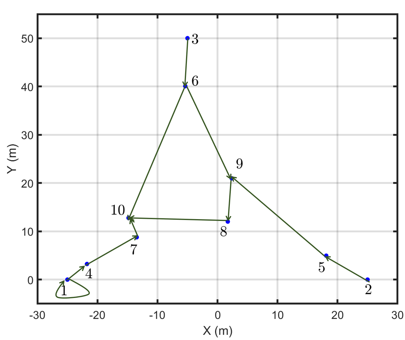
For cooperative coordination, the MAS uses the graph shown in Fig. 3 with the mobile robots located at their initial positions. Figure 4 shows is the graph used in cooperative localization, which is mainly based on proximity. The graph implies that leader agent is capable of self measurement while agents can measure the relative positions of agents . Meanwhile agent simultaneously measures the relative positions of agents , , and .
Since mobile robots are represented as double integrators, we must include process noise in the model to account for unmodeled dynamics. Hence we assume the standard deviation of the process noise to be . We also assume that the measurements obtained by all agents are polluted by additive Gaussian noise with a standard deviation of . In addition, all measurements are updated at a rate of .
The minimum time determined from (35) which satisfies conditions (31), (32), and (34) for this scenario is determined to be only assuming continuous noise-free full-state feedback. However, the minimum time is increased to when states are estimated using cooperative localization, as determined by optimization and verified via Monte Carlo simulations. In these simulations, the gains for the control law in (10) were selected as , . The selected safety threshold values were and .
Figure 5 shows the paths of the 10 mobile robots in the simulation. Figure 6 shows the global position estimation errors in and directions for a typical simulation with cooperative localization. Figure 7 shows the coordination tracking errors in and directions. It can be concluded that the both estimation and tracking errors never exceed of the distance travelled by each agent.


VIII Conclusion
This paper studied the problem of continuum deformation coordination using cooperative localization. The problem was presented as a decentralized leader follower coordination, where leaders’ desired trajectories and travel time between the initial and final configurations are obtained by solving coupled optimization problem. More specifically, leaders’ desired trajectories are determined by solving a constrained optimal control problem while the final time is minimized such that all safety requirements are satisfied. We also showed how follower agents can acquire the desired continuum deformation coordination through simultaneous communication and localization. As a result, a relatively-large number of agents of a multi-agent system can acquire a desired continuum deformation with low computation cost while all safety requirements are met and the MAS is capable of aggressive deformation in the geometrically-constrained environments.
Acknowledgment
This research was supported in part by the National Science Foundation under Award No. 1914581 and the Office of Naval Research under Award No. N00014-19-1-2255.
References
- [1] S. S. Kia, S. Rounds, and Sonia Martinez, “Cooperative Localization for Mobile Agents,” IEEE Control Systems Magazine, vol. 36, no. 2, pp. 86–101, 2016.
- [2] S. S. Kia, J. Hechtbauer, D. Gogokhiya, and S. Martinez, “Server-Assisted Distributed Cooperative Localization over Unreliable Communication Links,” IEEE Transactions on Robotics, vol. 34, no. 5, pp. 1392–1399, 2018.
- [3] S. I. Roumeliotis and G. A. Bekey, “Distributed multirobot localization,” IEEE Transactions on Robotics and Automation, vol. 18, no. 5, pp. 781–795, 2002.
- [4] H. Rastgoftar, Continuum deformation of multi-agent systems. Springer, 2016.
- [5] ——, “Fault-resilient continuum deformation coordination,” IEEE Transactions on Control of Network Systems, 2020.
- [6] H. Liu, L. Cheng, M. Tan, and Z.-G. Hou, “Containment control of continuous-time linear multi-agent systems with aperiodic sampling,” Automatica, vol. 57, pp. 78–84, 2015.
- [7] D. Wang and W. Wang, “Necessary and sufficient conditions for containment control of multi-agent systems with time delay,” Automatica, vol. 103, pp. 418–423, 2019.
- [8] M. Ji, G. Ferrari-Trecate, M. Egerstedt, and A. Buffa, “Containment control in mobile networks,” IEEE Transactions on Automatic Control, vol. 53, no. 8, pp. 1972–1975, 2008.
- [9] B. Li, Z.-q. Chen, Z.-x. Liu, C.-y. Zhang, and Q. Zhang, “Containment control of multi-agent systems with fixed time-delays in fixed directed networks,” Neurocomputing, vol. 173, pp. 2069–2075, 2016.
- [10] Q. Xiong, P. Lin, W. Ren, C. Yang, and W. Gui, “Containment control for discrete-time multiagent systems with communication delays and switching topologies,” IEEE transactions on cybernetics, vol. 49, no. 10, pp. 3827–3830, 2018.
- [11] F.-Y. Wang, Y.-H. Ni, Z.-X. Liu, and Z.-Q. Chen, “Containment control for general second-order multiagent systems with switched dynamics,” IEEE transactions on cybernetics, vol. 50, no. 2, pp. 550–560, 2018.
- [12] Z. Meng, W. Ren, and Z. You, “Distributed finite-time attitude containment control for multiple rigid bodies,” Automatica, vol. 46, no. 12, pp. 2092–2099, 2010.
- [13] Y. Zhao and Z. Duan, “Finite-time containment control without velocity and acceleration measurements,” Nonlinear Dynamics, vol. 82, no. 1-2, pp. 259–268, 2015.
- [14] X. He, Q. Wang, and W. Yu, “Finite-time containment control for second-order multiagent systems under directed topology,” IEEE Transactions on Circuits and Systems II: Express Briefs, vol. 61, no. 8, pp. 619–623, 2014.
- [15] X. Mu and K. Liu, “Containment control of single-integrator network with limited communication data rate,” IEEE Transactions on Automatic Control, vol. 61, no. 8, pp. 2232–2238, 2015.
- [16] H. Rastgoftar and E. M. Atkins, “Cooperative aerial lift and manipulation (calm),” Aerospace Science and Technology, vol. 82, pp. 105–118, 2018.