跳到论文正文
W Papers独立论文阅读器 arXiv:2104.09763 论文正文 计算阅读时间 · 0%
引用这篇论文根据当前论文元数据生成,正式投稿前建议核对。


License: arXiv.org perpetual non-exclusive license
arXiv:2104.09763v4 [math-ph] 07 Mar 2022

A mathematical analysis of Casimir interactions I: The scalar fieldThanks: Supported by Leverhulme grant RPG-2017-329

Yan-Long Fang Address: School of Mathematics, University of Leeds, Leeds , Yorkshire, LS2 9JT, UK Email address: Y.L.Fang@leeds.ac.uk and Alexander Strohmaier Address: School of Mathematics, University of Leeds, Leeds , Yorkshire, LS2 9JT, UK Email address: a.strohmaier@leeds.ac.uk
Abstract.

Starting from the construction of the free quantum scalar field of mass m≥0m\geq 0 we give mathematically precise and rigorous versions of three different approaches to computing the Casimir forces between compact obstacles. We then prove that they are equivalent.

1. Introduction

Casimir interactions are forces between objects such as perfect conductors. They can be either understood as quantum fluctuations of the vacuum or as the total effect of van-der-Waals forces. Hendrik Casimir predicted and computed this effect in the special case of two planar conductors in 1948 using an infinite mode summation ([9]). This force was measured experimentally by Sparnaay about 10 years later [57]. Since then also more precise measurements have been performed with good agreement to the theoretical prediction of Casimir([6, 11, 20, 44]). Other geometric situations, such as for example the Casimir force between a sphere and a plane, were also considered in precision experiments [47, 53].

The classical way to compute Casimir forces, and indeed the way it was done by Casimir himself, is by performing a zeta function regularisation of the vacuum energy. This has been carried out for a number of particular geometric situations (see [7, 8, 18, 19, 38] and references therein). Since this method requires knowledge of the spectrum of the Laplace operator in order to perform the analytic continuation it has long been a very difficult problem to compute the Casimir force in a generic geometric situation even from a non-rigorous point of view. Already, it has been realised by quantum field theorists (see e.g. [4, 14, 15, 37, 58]) that the Casimir force can also be understood by considering the renormalised stress energy tensor of the electromagnetic field. This tensor is defined by comparing the induced vacuum states of the quantum field with boundary conditions and the free theory. Once the renormalised stress energy tensor is mathematically defined, the computation of the Casimir energy density becomes a problem of spectral geometry (see e.g. [25]) and numerical analysis. The renormalised stress energy tensor and its relation to the Casimir effect can be understood at the level of rigour of axiomatic algebraic quantum field theory. Currently this is still the subject of ongoing research in mathematical physics (see e.g. [13]) in particular when it comes to the effect in curved backgrounds and fields that are not scalar, or in situations when the objects move.

Recently progress was made in the non-rigorous numerical computation of Casimir forces between objects (see for example [36, 55, 56]). This approach uses a formalism that relates the Casimir energy to a determinant computed from boundary layer operators. Such determinant formulae result in finite quantities that do not require further regularisation and have been obtained and justified in the physics literature [2, 21, 24, 22, 23, 41, 42, 49, 51, 52]. This has not only resulted in more efficient numerical algorithms but also in various asymptotic formulae for the Casimir forces for large and small separations. Many of the justifications and derivations of these formulae are based on physics considerations of macroscopic properties of matter or of van der Waals forces. As such they often involve ill defined path integrals. From a mathematical point of view considerations that link the determinant formulae to the spectral approach initially taken by Casimir have been largely formal computations or involve ad-hoc cut-offs and regularisation procedures. We note that in the Appendix of [42] it is proved correctly that the Fredholm determinant in the final formula of the Casimir energy is well defined. Only recently a mathematical justification of these formulae was given in [34], relating it to the trace of a linear combination of powers of the Laplace operator. The determinant formulae are directly related to the multi-reflection expansion of Balian and Duplantier [1] that also yields a finite Casimir energy. We mention [43] in the mathematical literature where the Casimir energy of a piston configuration is expressed in terms of the zeta regularised Fredholm determinant of the Dirichlet to Neumann operator.

Summarising, we list several ways to compute the Casimir force acting on a compact object that have been proposed and carried out:

  • (1)

    Using a total energy obtained in some way by regularising the spectrally defined zeta function. This can be done either directly or by first considering a compact problem in a box and then taking the adiabatic limit.

  • (2)

    By integrating the renormalised stress energy tensor around any surface enclosing the object.

  • (3)

    Using formulae for the energy in terms of a determinant of boundary layer operator.

The list is non-exhaustive and other methods exist, such as for example the worldline approach (see e.g. [28] and references). Here we will restrict ourselves to the listed methods.

The aim of the present paper is to establish, in the case of finitely many compact objects, the precise mathematical meaning of each of the listed methods for the case of the scalar field and then prove that they give the same answer for the force (not necessarily for the energy). The main tool to achieve this will be the relative stress energy tensor. This tensor mimics the definition of the relative trace of [34] and seems to not have been defined or studied previously in the literature. Note that the renormalised stress tensor becomes unbounded and non-integrable [10, 15] near the boundaries of objects and this makes it unsuitable to compute the total energy component from the energy density T00T_{00}. In contrast, the relative stress energy tensor is smooth up to the obstacles and is much more regular when considering boundary variations. This relative stress energy tensor does not satisfy Dirichlet or Neumann boundary conditions and therefore integration by parts involves boundary contributions. The relative energy density can be defined entirely in terms of functional calculus of the Laplace operator. This relative energy density has been introduced in [34]. It was shown to be integrable and its integral can be interpreted as the trace of a certain operator. The main result of [34] states that this trace can be expressed as the determinant of an operator constructed from boundary layer operators, thus providing a rigorous justification of the method (3) linking it with method (1). To show the equivalence of methods (2) and (3) we must provide a formula for the variation of the relative energy when one of the objects is moved. To compute this variation we prove and use a special case of the Hadamard variation formula ([27, 31, 50]) adapted to the non-compact setting. We then show that as a consequence of this formula that the variation of the total energy equals the surface integral of the spatial components of the relative stress energy tensor (see Theorem 5.9). This surface integral is also equal to the surface integral over the renormalised tensor (see Theorem 5.10). We will now give a more precise formulation of our main result.
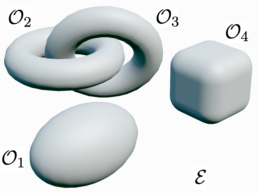
We consider dd-dimensional Euclidean space with d≥2d\geq 2. Let 𝒪\mathcal{O} be a bounded open subset of ℝd\mathbb{R}^{d} with smooth boundary such that the complement ℰ=ℝd∖𝒪¯\mathcal{E}=\mathbb{R}^{d}\setminus\overline{\mathcal{O}} is connected. The domain 𝒪\mathcal{O} will be assumed to consist of NN many connected components 𝒪1,…,𝒪N\mathcal{O}_{1},\ldots,\mathcal{O}_{N}. The space X=ℝd∖∂𝒪X=\mathbb{R}^{d}\setminus\partial\mathcal{O} therefore consists of the N+1N+1-many connected components 𝒪1,…,𝒪N,ℰ\mathcal{O}_{1},\ldots,\mathcal{O}_{N},\mathcal{E}. We think of 𝒪\mathcal{O} as obstacles placed in ℝd\mathbb{R}^{d}, and ℰ\mathcal{E} then corresponds to the exterior region of these obstacles. The set X⊂ℝdX\subset\mathbb{R}^{d} consists of the interior and the exterior of the obstacles, separated by ∂𝒪\partial\mathcal{O}. See Figure 1 for an example with three obstacles.
Refer to caption
Figure 1. Configuration of four obstacles 𝒪1,𝒪2,𝒪3,𝒪4\mathcal{O}_{1},\mathcal{O}_{2},\mathcal{O}_{3},\mathcal{O}_{4} with complement ℰ\mathcal{E} in a Euclidean space

For the free scalar field of mass m≥0m\geq 0 let TrenT_{\mathrm{ren}} be the renormalised stress energy tensor as defined in Section 2.2. In QFT terms this stress energy tensor is equivalent to the usual stress energy tensor obtained from canonical quantisation when normal ordering is used with respect to the free vacuum state. This is a smooth symmetric two-tensor away from ∂𝒪\partial\mathcal{O}, but it is singular at ∂𝒪\partial\mathcal{O} and the integral of T00T_{00} over ℰ\mathcal{E} does not converge. Let TrelT_{\mathrm{rel}} be the relative stress energy tensor as given in Definition 3.3. The relative total energy ErelE_{\mathrm{rel}} is defined as the integral of (Trel)00​(x)(T_{\mathrm{rel}})_{00}(x) over ℝd\mathbb{R}^{d} which can be shown to exist and to be equal the trace of a certain combination of operators. In case m>0m>0 the regularised energy EregE_{\mathrm{reg}} is defined in Section 6, Definition 6.3 via zeta function regularisation. We would like to compute the force on an object 𝒪j\mathcal{O}_{j} due to the presence of the other objects. Approach (2) is to directly compute

Fi=∫Σ(Tren)i​k​nk​𝑑σF_{i}=\int_{\Sigma}(T_{\mathrm{ren}})_{ik}n^{k}\mathrm{d}\sigma

where TrenT_{\mathrm{ren}} is the renormalised stress energy tensor given in Definition 2.3 and Σ\Sigma is any smooth surface enclosing 𝒪j\mathcal{O}_{j} (i.e. homologous to ∂𝒪j\partial\mathcal{O}_{j} in ℰ¯\overline{\mathcal{E}}), nkn^{k} is the exterior unit normal vector field, and d​σ\mathrm{d}\sigma is the surface measure on Σ\Sigma. If energy conservation holds, i.e. no energy is radiated off to infinity, one expects this force to be the directional derivative of the total energy when 𝒪j\mathcal{O}_{j} is moved rigidly. Thus, let ZZ be a constant vector field on ℝd\mathbb{R}^{d}. Let YY be a vector field that equals ZZ near 𝒪j\mathcal{O}_{j} and vanishes near 𝒪l\mathcal{O}_{l} when l≠jl\not=j. The vector field generates a flow Φϵ\Phi_{\epsilon} that, for ϵ\epsilon near zero, moves the object 𝒪j\mathcal{O}_{j} rigidly and we end up with a configuration that depends on the parameter ϵ\epsilon. The total energies ErelE_{\mathrm{rel}} and EregE_{\mathrm{reg}} then also depend on ϵ\epsilon in that way and become functions of ϵ\epsilon in a small interval around zero. The change of these energies with respect to the flow can be interpreted as the change of energy needed to move object 𝒪j\mathcal{O}_{j} rigidly relative to the other objects in the direction of ZZ. Our main result may be stated as follows.

Theorem 1.1.

The relative energy Erel​(ϵ)E_{\mathrm{rel}}(\epsilon) is differentiable in ϵ\epsilon at ϵ=0\epsilon=0 and its derivative equals Fi​ZiF_{i}Z^{i}, where

(1) Fi=∫Σ(Trel)i​k​nk​𝑑σ=∫Σ(Tren)i​k​nk​𝑑σ.F_{i}=\int_{\Sigma}(T_{\mathrm{rel}})_{ik}n^{k}\mathrm{d}\sigma=\int_{\Sigma}(T_{\mathrm{ren}})_{ik}n^{k}\mathrm{d}\sigma.

Moreover,

(2) Erel=12​π​∫m∞ωω2−m2​log​detQrel​(ω)​𝑑ω,E_{\mathrm{rel}}=\frac{1}{2\pi}\int_{m}^{\infty}\frac{\omega}{\sqrt{\omega^{2}-m^{2}}}\log\det Q_{\mathrm{rel}}(\omega)\mathrm{d}\omega,

where Qrel​(ω)=Qi​ω​(Q~i​ω)−1Q_{\mathrm{rel}}(\omega)=Q_{\mathrm{i}\omega}(\tilde{Q}_{\mathrm{i}\omega})^{-1} is defined in detail in Section 3 and constructed out of boundary layer operators for the Laplacian. If m>0m>0 then Erel​(ϵ)−Ereg​(ϵ)E_{\mathrm{rel}}(\epsilon)-E_{\mathrm{reg}}(\epsilon) is constant near ϵ=0\epsilon=0.

We note that this mathematical theorem simply shows that all these proposed computational methods give the same Casimir interactions in the case of separated rigid bodies. The statement does not say anything about the actual origin of the Casimir force or its existence, which needs to be determined from experiments or physics considerations. There is however a strong argument for the expression

Fi=∫Σ(Trel)i​k​nk​𝑑σF_{i}=\int_{\Sigma}(T_{\mathrm{rel}})_{ik}n^{k}\mathrm{d}\sigma

to be a directly relevant physical quantity. Our point of view is that the stress energy tensor does not have an absolute meaning in this context, but rather is used to compare two vacuum states (normal ordering depends on a comparison state). If we would like to know the effect for the rigid objects 𝒪2,…​𝒪N\mathcal{O}_{2},\ldots\mathcal{O}_{N} on the rigid object 𝒪1\mathcal{O}_{1} the states to compare are not the ground state with Dirichlet conditions and the free ground state. It is rather the vacuum states obtained from the Laplacian with Dirichlet conditions imposed on 𝒪1\mathcal{O}_{1} alone and with Dirichlet conditions on all the objects. The comparison of these two states yields a stress energy tensor that is completely regular near 𝒪1\mathcal{O}_{1}, and the computation of the force based on this tensor leads directly to the above formula without regularisation.

The paper is organised as follows. In Section 2 we review the rigorous construction of the free scalar field of mass m≥0m\geq 0 in the presence of boundaries and show how this leads to a natural definition of the renormalised stress energy tensor, which is given in Section 2.2. We also review its most important properties and express it in terms of spectral quantities for the Laplace operator. Section 3 introduces the relative setting and gives the definition of the relative stress energy tensor and its basic properties. Some norm estimates on the relative resolvent are given in Section 4, which provides mathematical justifications for later proofs. In Section 5 we prove a Hadamard variation formula and compute the variation of the relative energy to establish the first part of the main theorem. In Section 6 we show that for m>0m>0 the renormalised version of the zeta function has a meromorphic continuation and can thus be used to define the regularised energy. This section also contains a proof that variations of the regularised energy and the relative energy coincide. To illustrate the method and relate it to the classical computations we treat the easier example of the one-dimensional Casimir energy explicitly in Appendix B. This example also illustrates that a divergence term for the time-component of the renormalised stress energy tensor that is normally neglected needs to be taken into account to obtained the correct result (see Remark 2.5).

In a follow-up paper we will establish a similar theorem for the electromagnetic field. We note here that the stress energy for the electromagnetic field is quite different from the scalar field and there are additional complications such as zero modes ([60]) that are absent for the scalar field. Moreover, the boundary conditions for the electromagnetic field are slightly more complicated, and cannot be reduced to Dirichlet boundary conditions. We therefore decided to not attempt a unified treatment which would obscure the result by additional notations.

Our approach is expected to carry over to other boundary conditions such a Neumann, mixed Dirichlet-Neumann, or Robin boundary conditions with the single layer operators replaced by the appropriate layer operators. As in the electromagnetic case additional technical problems need to be overcome in these cases due to the possible appearance of zero modes and singularities of the Dirichlet-to-Neumann map at zero.

1.1. Notations

Let M⊂ℝdM\subset\mathbb{R}^{d} be an open subset. By the Schwartz kernel theorem continuous linear operators A:C0∞​(M)→𝒟′​(M)A:C^{\infty}_{0}(M)\to\mathcal{D}^{\prime}(M) are in one to one correspondence to distributions in 𝒟′​(M×M)\mathcal{D}^{\prime}(M\times M), i.e. for every such AA there exists a unique Schwartz kernel in 𝒟′​(M×M)\mathcal{D}^{\prime}(M\times M). In this paper the Schwartz kernel of AA will be denoted by A˘\breve{A}.

2. Scalar quantum field theory with Dirichlet boundary conditions

Let −Δ-\Delta be the (positive) Dirichlet Laplacian imposed on the codimension one submanifold ∂𝒪\partial\mathcal{O}. By definition this is the unbounded self-adjoint operator defined on the Hilbert space L2​(ℝd)L^{2}(\mathbb{R}^{d}) associated with the Dirichlet quadratic form qD​(f,f)=∫X‖∇f‖2​𝑑xq_{D}(f,f)=\int_{X}\|\nabla f\|^{2}\mathrm{d}x with form-domain being the Sobolev space H01​(X)H^{1}_{0}(X).

As a consequence of elliptic regularity ([59]*Section 7.2) we have for the domain of dom⁡((−Δ)s2)\mathrm{dom}((-\Delta)^{\frac{s}{2}}) equipped with its graph norm for any s∈2​ℕ0s\in 2\mathbb{N}_{0} the continuous inclusions

Hcomps​(X)⊂dom⁡((−Δ)s2)⊂Hlocs​(X).H^{s}_{\mathrm{comp}}(X)\subset\mathrm{dom}((-\Delta)^{\frac{s}{2}})\subset H^{s}_{\mathrm{loc}}(X).

One can use complex interpolation ([63]*§4 and Theorem 4.2) to extend this to any s≥0s\geq 0. Here Hcomps​(X)H^{s}_{\mathrm{comp}}(X) denotes the space of functions in Hs​(X)H^{s}(X) with compact support in XX.

The Hilbert space L2​(ℝd)L^{2}(\mathbb{R}^{d}) then decomposes into a direct sum

L2​(ℝd)=L2​(𝒪1)⊕…⊕L2​(𝒪N)⊕L2​(ℰ)L^{2}(\mathbb{R}^{d})=L^{2}(\mathcal{O}_{1})\oplus\ldots\oplus L^{2}(\mathcal{O}_{N})\oplus L^{2}(\mathcal{E})

and each subspace is an invariant subspace for −Δ-\Delta in the sense that any bounded function of the operator as defined by spectral calculus will leave these subspaces invariant. The restriction of −Δ-\Delta to L2​(𝒪j)L^{2}(\mathcal{O}_{j}) is the Dirichlet Laplacian on the interior of 𝒪j\mathcal{O}_{j} and therefore has compact resolvent. The restriction of −Δ-\Delta to L2​(ℰ)L^{2}(\mathcal{E}) has purely absolutely continuous spectrum [0,∞)[0,\infty). By comparison we also have the free Laplacian −Δfree-\Delta_{\textrm{free}} on ℝd\mathbb{R}^{d} which corresponds to the case 𝒪=∅\mathcal{O}=\emptyset. Throughout the paper we fix a mass parameter m≥0m\geq 0.

Definition 2.1.

The relativistic Hamiltonian HH is defined to be the self-adjoint operator H=(−Δ+m2)12H=(-\Delta+m^{2})^{\frac{1}{2}}.

The space-time MM we consider is the Lorentzian spacetime ℝ×X\mathbb{R}\times X with Minkowski metric. The forward and backward fundamental solutions G+/−:C0∞(M)→C∞(M)G_{+/-}:C^{\infty}_{0}(M)\to C^{\infty}(M) of the Klein-Gordon operator □+m2\Box+m^{2} with Dirichlet boundary conditions are given by

(G+​f)​(t,x)=∫(θ⁡(t−t′)​H−1​sin⁡(H⁡(t−t′))​f​(t′,⋅))​(x)​d​t′,\displaystyle(G_{+}f)(t,x)=\int\left(\theta(t-t^{\prime})H^{-1}\sin(H(t-t^{\prime}))f(t^{\prime},\cdot)\right)(x)\mathrm{d}t^{\prime},
(G−​f)​(t,x)=∫(θ⁡(t′−t)​H−1​sin⁡(H⁡(t′−t))​f​(t′,⋅))​(x)​d​t′,\displaystyle(G_{-}f)(t,x)=\int\left(\theta(t^{\prime}-t)H^{-1}\sin(H(t^{\prime}-t))f(t^{\prime},\cdot)\right)(x)\mathrm{d}t^{\prime},

where θ\theta is the Heaviside step function. As usual in canonical quantisation one considers the difference G=G+−G−G=G_{+}-G_{-} given by

(G​f)​(t,x)=∫(H−1​sin⁡(H⁡(t−t′))​f​(t′,⋅))​(x)​d​t′.\displaystyle(Gf)(t,x)=\int\left(H^{-1}\sin(H(t-t^{\prime}))f(t^{\prime},\cdot)\right)(x)\mathrm{d}t^{\prime}.

Here H−1​sin⁡(H⁡(t−t′))H^{-1}\sin(H(t-t^{\prime})) is defined by spectral calculus. Since the function |x−1​sin⁡(x​t)||x^{-1}\sin(xt)| is bounded by |t||t| the operator H−1​sin⁡(H⁡(t−t′))H^{-1}\sin(H(t-t^{\prime})) defines for any s≥0s\geq 0 a bounded map from Hcomps​(X)H^{s}_{\mathrm{comp}}(X) to dom​(−Δ)s⊂Hs​(𝒪1)⊕…​Hs​(𝒪N)⊕Hs​(ℰ)\mathrm{dom}(-\Delta)^{s}\subset H^{s}(\mathcal{O}_{1})\oplus\ldots H^{s}(\mathcal{O}_{N})\oplus H^{s}(\mathcal{E}). Here the inclusion of the domain in the Sobolev spaces follows for s∈2​ℕ0s\in 2\mathbb{N}_{0} from elliptic regularity up to the boundary ([48]*Theorem 4.18) and for general s≥0s\geq 0 by interpolation. In particular, this means that H−1​sin⁡(H⁡(t−t′))H^{-1}\sin(H(t-t^{\prime})) has a distributional integral kernel. We can define a symplectic structure σ\sigma on 𝒲=C0∞​(M)/((□+m2)​C0∞​(M))\mathcal{W}=C^{\infty}_{0}(M)/\left((\Box+m^{2})C^{\infty}_{0}(M)\right) by

σ⁡([f],[g])=(f,G​g).\sigma([f],[g])=(f,Gg).

This induces a symplectic structure on G​C0∞​(M)GC^{\infty}_{0}(M) that is well known to coincide with the standard symplectic structure on the space of solutions. Indeed, if we define u=G​fu=Gf and v=G​gv=Gg for f,g∈C0∞​(M)f,g\in C^{\infty}_{0}(M) then uu and vv solve the Klein-Gordon equation with Dirichlet boundary conditions and

(f,G​g)=∫X(∂tu)​v−(∂tv)​u​𝑑x.(f,Gg)=\int_{X}(\partial_{t}u)v-(\partial_{t}v)u\mathrm{d}x.

In this equality the right hand side is independent of tt.

2.1. Field algebra and the vacuum state

The field algebra of the real Klein-Gordon field is then the (unbounded) CCR ∗*-algebra of this symplectic space. Instead of using the symplectic space 𝒲\mathcal{W} one can describe this algebra 𝒜\mathcal{A} directly as the complex unital ∗*-algebra generated by symbols ϕ⁡(f)\phi(f) with f∈C0∞​(M,ℝ)f\in C^{\infty}_{0}(M,\mathbb{R}) satisfying the relation

f→ϕ⁡(f)is real linear,\displaystyle f\to\phi(f)\quad\textrm{is real linear},
[ϕ⁡(f1),ϕ⁡(f2)]=−i⁡(f1,G​f2)​𝟏\displaystyle[\phi(f_{1}),\phi(f_{2})]=-\mathrm{i}(f_{1},Gf_{2})\mathbf{1}
ϕ​(f)∗=ϕ⁡(f),\displaystyle\phi(f)^{*}=\phi(f),
ϕ⁡((□+m2)​f)=0.\displaystyle\phi((\Box+m^{2})f)=0.

Physical states of this quantum system are states on this ∗*-algebra. The construction and physical interpretations of such states usually relies on a Fock representation of 𝒜\mathcal{A}. This representation is chosen on physical grounds as a positive energy representation.

We briefly explain this now. The group of time translations (Ts​f)​(t,x)=f⁡(t−s,x)(T_{s}f)(t,x)=f(t-s,x) commutes with □+m2\Box+m^{2} and GG and therefore αt​(ϕ⁡(f)):=ϕ⁡(Tt​f)\alpha_{t}(\phi(f)):=\phi(T_{t}f) defines a group of ∗*-automorphisms of 𝒜\mathcal{A}. If a state ω:𝒜→ℂ\omega:\mathcal{A}\to\mathbb{C} is invariant then this group lifts to a group of unitary transformations U⁡(t)U(t) on the GNS-Hilbert space which is uniquely determined by

π⁡(αt​(a))=Ut​π​(a)​U−t,\displaystyle\pi(\alpha_{t}(a))=U_{t}\pi(a)U_{-t},
Ut​Ω=Ω.\displaystyle U_{t}\Omega=\Omega.

We say that π\pi is a positive energy representation if this group is strongly continuous and its infinitesimal generator has non-negative spectrum.

We will focus in this paper on the quasi-free ground state. This means that the state is completely determined by its two point distribution

ω2∈𝒟′​(M×M),ω2​(f1⊗f2)=ω⁡(ϕ⁡(f1)​ϕ​(f2))\omega_{2}\in\mathcal{D}^{\prime}(M\times M),\quad\omega_{2}(f_{1}\otimes f_{2})=\omega\left(\phi(f_{1})\phi(f_{2})\right)

which is given explicitly as

ω2​(f1⊗f2)=∫ℝ×ℝ(f1​(t,⋅),12​H−1​e−i​H​(t−t′)​f2​(t′,⋅))​𝑑t​d​t′,\omega_{2}(f_{1}\otimes f_{2})=\int_{\mathbb{R}\times\mathbb{R}}(f_{1}(t,\cdot),\frac{1}{2}H^{-1}e^{-\mathrm{i}H(t-t^{\prime})}f_{2}(t^{\prime},\cdot))\>\mathrm{d}t\;\mathrm{d}t^{\prime},

i.e. ω2\omega_{2} is the integral kernel of the operator H−1​e−i​H​(t−t′)H^{-1}e^{-\mathrm{i}H(t-t^{\prime})}. In case m=0m=0 the spectrum of HH contains zero and this expression needs to be interpreted in the sense of quadratic forms. Namely, it follows from general resolvent expansions (for example [60]*Theorem 1.5, 1.6 and 1.7) that C0∞​(X)C^{\infty}_{0}(X) is contained in the domain of the operator H−12H^{-\frac{1}{2}}. This follows from the formula

⟨H−12​f,H−12​f⟩=2π​∫0∞⟨(−Δ+λ2)−1​f,f⟩​𝑑λ.\langle H^{-\frac{1}{2}}f,H^{-\frac{1}{2}}f\rangle=\frac{2}{\pi}\int_{0}^{\infty}\langle(-\Delta+\lambda^{2})^{-1}f,f\rangle\mathrm{d}\lambda.

In particular, the space of test functions C0∞​(X)C^{\infty}_{0}(X) is contained in the form domain of H−1H^{-1} and therefore, by the Schwartz kernel theorem, the operator H−1H^{-1} has a distributional kernel in 𝒟′​(X×X)\mathcal{D}^{\prime}(X\times X). This is of course also the case for general m>0m>0. We will denote the integral kernel of H−1H^{-1} by H˘−1\breve{H}^{-1}, mildly abusing notation.

One can check directly that ω2\omega_{2} defines a positive energy representation. Instead of using −Δ-\Delta we could also have used −Δfree-\Delta_{\textrm{free}}, the free Laplace operator. This also defines a positive energy state on the free algebra of observables 𝒜free\mathcal{A}_{\textrm{free}} which we will denote by ωfree\omega_{\textrm{free}}, and similarly we use the notation Hfree=(−Δfree+m2)12H_{\textrm{free}}=(-\Delta_{\textrm{free}}+m^{2})^{\frac{1}{2}}. There states can be compared by restricting them to certain subalgebras that are contained in both the algebra of observables and the free algebra of observables. For example if UU is contained in a double cone in MM then 𝒜⁡(U)\mathcal{A}(U) which is generated by ϕ⁡(f),supp⁡(f)⊂U\phi(f),\mathrm{supp}(f)\subset U can be thought of as a subset of both 𝒜\mathcal{A} and 𝒜free\mathcal{A}_{\textrm{free}} and therefore both states can be restricted to this algebra.

2.2. The renormalised stress-energy tensor

The classical stress energy tensor of the Klein-Gordon field for a smooth real-valued solution uu is given by

Tc​l​(u)=d​u⊗d​u−12​g​(d​u,d​u)​g−12​g​m2​u2.T^{cl}(u)=\mathrm{d}u\otimes\mathrm{d}u-\frac{1}{2}g(\mathrm{d}u,\mathrm{d}u)g-\frac{1}{2}g\,m^{2}u^{2}.

This is a symmetric 22-tensor on MM and one can easily show, using the Klein-Gordon equation, that it is divergence-free. Here gg is the Minkowski metric on MM with signature (−1,1,…,1)(-1,1,\ldots,1). The Euclidean metric on ℝd\mathbb{R}^{d} will be denoted by hh. The components Ti​jc​lT_{ij}^{cl} of the stress energy tensor are the restrictions to the diagonal of the functions Qi​jc​l​(x,y)Q^{cl}_{ij}(x,y) defined on M×MM\times M by

Qi​jc​l​(x,y)=(∇iu)​(x)⊗(∇ju)​(y)−12​gi​j​(∇ku)​(x)⋅∇ku​(y)−12​gi​j​m2​u​(x)​u​(y).Q^{cl}_{ij}(x,y)=(\nabla_{i}u)(x)\otimes(\nabla_{j}u)(y)-\frac{1}{2}g_{ij}(\nabla_{k}u)(x)\cdot\nabla^{k}u(y)-\frac{1}{2}g_{ij}m^{2}u(x)u(y).

The quantum field theory counterpart of QQ can be written in the field algebra as a field-algebra-valued bilinear form in the test functions f1,f2∈C∞​(M)f_{1},f_{2}\in C^{\infty}(M) as

Qi​j​(f1⊗f2)=ϕ⁡(∇if1)​ϕ​(∇jf2)−12​ϕ​(∇kf1)​ϕ​(∇kf2)​gi​j−12​gi​j​m2​ϕ​(f1)​ϕ​(f2).Q_{ij}(f_{1}\otimes f_{2})=\phi(\nabla_{i}f_{1})\phi(\nabla_{j}f_{2})-\frac{1}{2}\phi(\nabla_{k}f_{1})\phi(\nabla^{k}f_{2})g_{ij}-\frac{1}{2}g_{ij}m^{2}\phi(f_{1})\phi(f_{2}).

The expectation value of Qi​jQ_{ij} with respect to the state ω\omega is then given in terms of the two point function ω2\omega_{2} as

ω⁡(Qi​j)​(f1,f2)=ω2​(∇if1⊗∇jf2−12​∇kf1⊗∇kf2​gi​j−12​gi​j​m2​f1⊗f2).\omega(Q_{ij})(f_{1},f_{2})=\omega_{2}(\nabla_{i}f_{1}\otimes\nabla_{j}f_{2}-\frac{1}{2}\nabla_{k}f_{1}\otimes\nabla^{k}f_{2}g_{ij}-\frac{1}{2}g_{ij}m^{2}f_{1}\otimes f_{2}).

Let K⁡(t,x,y)K(t,x,y) be the distributional kernel of 12​H−1​e−i​H​t\frac{1}{2}H^{-1}e^{-\mathrm{i}Ht}. Then the distribution ω⁡(Qi​j)\omega(Q_{ij}) with respect to the ground state is given by

{ω(Q00)(t,t′,x,x′)=12(∂t∂t′+∑k=1d∂xk∂x′k+m2)K(t−t′,x,x′)ω(Q0​i)(t,t′,x,x′)=(∂t′∂xi)K(t−t′,x,x′)for1≤i≤dω(Qi​j)(t,t′,x,x′)=(∂x′i∂xj)K(t−t′,x,x′)fori≠jand1≤i,j≤dω(Qi​i)(t,t′,x,x′)=12(∂t∂t′+∂xi∂x′i−∑k≠id∂xk∂x′k−m2)K(t−t′,x,x′)for1≤i≤d\left\{\begin{aligned} &\omega(Q_{00})(t,t^{\prime},x,x^{\prime})=\frac{1}{2}\left(\partial_{t}\partial_{t^{\prime}}+\sum_{k=1}^{d}\partial_{x^{k}}\partial_{x^{\prime k}}+m^{2}\right)K(t-t^{\prime},x,x^{\prime})\\ &\omega(Q_{0i})(t,t^{\prime},x,x^{\prime})=\left(\partial_{t^{\prime}}\partial_{x^{i}}\right)K(t-t^{\prime},x,x^{\prime})\quad\text{for}\quad 1\leq i\leq d\\ &\omega(Q_{ij})(t,t^{\prime},x,x^{\prime})=\left(\partial_{x^{\prime i}}\partial_{x^{j}}\right)K(t-t^{\prime},x,x^{\prime})\quad\text{for}\quad i\neq j\quad\text{and}\quad 1\leq i,j\leq d\\ &\omega(Q_{ii})(t,t^{\prime},x,x^{\prime})=\frac{1}{2}\left(\partial_{t}\partial_{t^{\prime}}+\partial_{x^{i}}\partial_{x^{\prime i}}-\sum_{k\neq i}^{d}\partial_{x^{k}}\partial_{x^{\prime k}}-m^{2}\right)K(t-t^{\prime},x,x^{\prime})\quad\text{for}\quad 1\leq i\leq d\end{aligned}\right.

or in short,

(3) ω(Qi​j)(t,t′,x,x′)=[∂i′∂jK−12gi​j(∂k′∂k+m2)K](t−t′,x,x′).\omega(Q_{ij})(t,t^{\prime},x,x^{\prime})=\left[\partial_{i}^{\prime}\partial_{j}K-\frac{1}{2}g_{ij}(\partial_{k}^{\prime}\partial^{k}+m^{2})K\right](t-t^{\prime},x,x^{\prime}).

The above expressions are formal and make sense only when paired with test functions. We will use such formal notation throughout the paper when there is danger of confusion. The expectation value of the stress energy tensor would correspond to the restriction of ω⁡(Qi​j)\omega(Q_{ij}) to the diagonal as a distribution. Unfortunately, the distribution ω⁡(Qi​j)\omega(Q_{ij}) is singular and cannot be restricted to the diagonal in a straightforward manner. If one is interested in relative quantities only then one can still define the renormalised expectation value of the stress energy tensor between the states. Both states ω\omega and ωfree\omega_{\textrm{free}} are positive energy states and therefore satisfy the Hadamard condition (for example [61]*Theorem 6.3). By uniqueness of such Hadamard states the difference of the two-point distributions is smooth near the diagonal in M×MM\times M. In the present case this can also be seen more directly as follows. Let Kfree​(t,x,y)K_{\textrm{free}}(t,x,y) be the kernel of 12​Hfree−1​e−i​Hfree​t\frac{1}{2}H_{\textrm{free}}^{-1}e^{-\mathrm{i}H_{\textrm{free}}t}. We will consider the difference 𝒦⁡(t,x,y)=K⁡(t,x,y)−Kfree​(t,x,y)\mathcal{K}(t,x,y)=K(t,x,y)-K_{\textrm{free}}(t,x,y).

Theorem 2.2.

The distribution 𝒦\mathcal{K} is smooth near the set {(0,x,y)∣x,y∈X}⊂ℝ×X×X\{(0,x,y)\mid x,y\in X\}\subset\mathbb{R}\times X\times X. In particular H˘−1−H˘free−1\breve{H}^{-1}-\breve{H}^{-1}_{\textrm{free}} is smooth in X×XX\times X.

Proof.

The distribution 𝒦⁡(t,x,y)\mathcal{K}(t,x,y) is a solution of the wave equation

∂t2−12(Δx+Δy)𝒦(t,x,y)=0\partial_{t}^{2}-\frac{1}{2}\left(\Delta_{x}+\Delta_{y}\right)\mathcal{K}(t,x,y)=0

on ℝ×X×X\mathbb{R}\times X\times X with initial conditions

𝒦⁡(0,x,y)=12​(H˘−1​(x,y)−H˘free−1​(x,y)),\displaystyle\mathcal{K}(0,x,y)=\frac{1}{2}\left(\breve{H}^{-1}(x,y)-\breve{H}^{-1}_{\textrm{free}}(x,y)\right),
∂t𝒦⁡(t,x,y)|t=0=0.\displaystyle\partial_{t}\mathcal{K}(t,x,y)|_{t=0}=0.

By [34]*Lemma 5.1 integral kernel κλ\kappa_{\lambda} of the resolvent difference

(−Δ+λ2)−1−(−Δfree+λ2)−1(-\Delta+\lambda^{2})^{-1}-(-\Delta_{\textrm{free}}+\lambda^{2})^{-1}

is smooth and satisfies on any compact subset UU of X×XX\times X a CkC^{k}-norm bound of the form

(4) ‖κλ‖Ck​(U)≤Ck,U​|log⁡(|λ|)|ℓ​e−δ′​λ​ for all ​λ>0\displaystyle\|\kappa_{\lambda}\|_{C^{k}(U)}\leq C_{k,U}|\log(|\lambda|)|^{\ell}e^{-\delta^{\prime}\lambda}\textrm{ for all }\lambda>0

for some ℓ≥0\ell\geq 0 and δ′>0\delta^{\prime}>0. Therefore the integral representation

H−1−Hfree−1=2π​∫m∞λλ2−m2​κλ​𝑑λH^{-1}-H^{-1}_{\textrm{free}}=\frac{2}{\pi}\int_{m}^{\infty}\frac{\lambda}{\sqrt{\lambda^{2}-m^{2}}}\kappa_{\lambda}\mathrm{d}\lambda

converges in the C∞​(X×X)C^{\infty}(X\times X) topology. Thus the distribution H˘−1−H˘free−1\breve{H}^{-1}-\breve{H}^{-1}_{\textrm{free}} is smooth in X×XX\times X. Since the initial conditions are smooth the solution 𝒦\mathcal{K} is smooth where it is uniquely determined by the initial data. This is the case in a neighborhood of t=0t=0 in ℝ×X×X\mathbb{R}\times X\times X. ∎

Hence the distribution ω⁡(Qi​j)−ωfree​(Qi​j)\omega(Q_{ij})-\omega_{\textrm{free}}(Q_{ij}) is a smooth function in a neighbourhood of the diagonal Δ⊂M×M\mathtt{\Delta}\subset M\times M.

Definition 2.3.

The components (Tren)i​j(T_{\mathrm{ren}})_{ij} of the renormalised stress energy tensor TrenT_{\mathrm{ren}} are defined to be the restriction to the diagonal of the function ω⁡(Qi​j)−ωfree​(Qi​j)\omega(Q_{ij})-\omega_{\textrm{free}}(Q_{ij}).

Theorem 2.4.

The renormalised stress energy tensor is symmetric and is given by

(5) {(Tren)00=12​(H˘−H˘free)|Δ+18​Δ​[(H˘−1−H˘free−1)|Δ](Tren)i​j=12​[∂i∂j′(H˘−1−H˘free−1)]|Δ−18​hi​j​Δ​[(H˘−1−H˘free−1)|Δ](Tren)0​i=0\left\{\begin{aligned} &(T_{\mathrm{ren}})_{00}=\frac{1}{2}(\breve{H}-\breve{H}_{\textrm{free}})|_{\mathtt{\Delta}}+\frac{1}{8}\Delta[(\breve{H}^{-1}-\breve{H}_{\textrm{free}}^{-1})|_{\mathtt{\Delta}}]\\ &(T_{\mathrm{ren}})_{ij}=\frac{1}{2}[\partial_{i}\partial_{j}^{\prime}(\breve{H}^{-1}-\breve{H}_{\textrm{free}}^{-1})]|_{\mathtt{\Delta}}-\frac{1}{8}h_{ij}\Delta[(\breve{H}^{-1}-\breve{H}_{\textrm{free}}^{-1})|_{\mathtt{\Delta}}]\\ &(T_{\mathrm{ren}})_{0i}=0\end{aligned}\right.

and

{(Tren)00=12​(H˘−H˘free)|Δ+18​Δ​[(H˘−1−H˘free−1)|Δ](Tren)i​j=−12​[∂i∂j(H˘−1−H˘free−1)]|Δ+14​∂i∂j[(H˘−1−H˘free−1)|Δ]−18​hi​j​Δ​[(H˘−1−H˘free−1)|Δ](Tren)0​i=0\left\{\begin{aligned} &(T_{\mathrm{ren}})_{00}=\frac{1}{2}(\breve{H}-\breve{H}_{\textrm{free}})|_{\mathtt{\Delta}}+\frac{1}{8}\Delta[(\breve{H}^{-1}-\breve{H}_{\textrm{free}}^{-1})|_{\mathtt{\Delta}}]\\ &(T_{\mathrm{ren}})_{ij}=-\frac{1}{2}[\partial_{i}\partial_{j}(\breve{H}^{-1}-\breve{H}_{\textrm{free}}^{-1})]|_{\mathtt{\Delta}}+\frac{1}{4}\partial_{i}\partial_{j}[(\breve{H}^{-1}-\breve{H}_{\textrm{free}}^{-1})|_{\mathtt{\Delta}}]-\frac{1}{8}h_{ij}\Delta[(\breve{H}^{-1}-\breve{H}_{\textrm{free}}^{-1})|_{\mathtt{\Delta}}]\\ &(T_{\mathrm{ren}})_{0i}=0\end{aligned}\right.

for 1≤i,j≤d1\leq i,j\leq d. Note that here H˘−1\breve{H}^{-1} and H˘free−1\breve{H}^{-1}_{\textrm{free}} are the the integral kernels of H−1H^{-1} and Hfree−1H^{-1}_{\textrm{free}} respectively. Moreover, the expression A˘|Δ\breve{A}|_{\mathtt{\Delta}} means the restriction of the integral kernel, A˘\breve{A}, to the diagonal (See Section 1.1).

Remark 2.5.

The terms of divergence forms in the renormalised stress energy tensor are commonly neglected in the literature, as one may naively think that they have zero contribution when integrating over the whole space. However, this is not the case. As it is not integrable due to the singular behaviour near the boundary, the divergence theorem does not apply in this case. See Appendix B for the simplest case. The problem disappears when we work with the relative stress energy tensor given in Definition 3.3.

Proof of Theorem 2.4.

Let 𝒦⁡(t,x,x′)\mathcal{K}(t,x,x^{\prime}) be the kernel of 12​(H−1​e−i​H​t−Hfree−1​e−i​Hfree​t)\frac{1}{2}(H^{-1}e^{-\mathrm{i}Ht}-H_{\textrm{free}}^{-1}e^{-\mathrm{i}H_{\textrm{free}}t}) and 𝒦⁡(t,t′,x,x′)=𝒦⁡(t−t′,x,x′)\mathscr{K}(t,t^{\prime},x,x^{\prime})=\mathcal{K}(t-t^{\prime},x,x^{\prime}). We have that

(6) (Tren)i​j=[∂i′∂j−12gi​j(∂k′∂k+m2)]𝒦|Δ,(T_{\mathrm{ren}})_{ij}=\left.\left[\partial_{i}^{\prime}\partial_{j}-\frac{1}{2}g_{ij}(\partial_{k}^{\prime}\partial^{k}+m^{2})\right]\mathscr{K}\right|_{\mathtt{\Delta}},

where ∂0=∂t\partial_{0}=\partial_{t}, ∂′0=∂t′\partial^{\prime}_{0}=\partial_{t^{\prime}}, ∂i=∂xi\partial_{i}=\partial_{x^{i}} and ∂i′=∂x′i\partial_{i}^{\prime}=\partial_{x^{\prime i}} for 1≤i≤d1\leq i\leq d. By theorem 2.2 the distribution 𝒦⁡(t,t′,x,x′)\mathscr{K}(t,t^{\prime},x,x^{\prime}) is smooth in a neighbourhood of the diagonal Δ⊂M×M\mathtt{\Delta}\subset M\times M. Moreover, 𝒦⁡(t−t′,⋅,⋅)\mathcal{K}(t-t^{\prime},\cdot,\cdot) is the kernel of a symmetric operator on XX with respect to the real inner product (⋅,⋅)(\cdot,\cdot) and therefore satisfies

(7) 𝒦⁡(t−t′,x,x′)=𝒦⁡(t,t′,x,x′)=𝒦⁡(t,t′,x′,x)=𝒦⁡(t−t′,x′,x).\mathcal{K}(t-t^{\prime},x,x^{\prime})=\mathscr{K}(t,t^{\prime},x,x^{\prime})=\mathscr{K}(t,t^{\prime},x^{\prime},x)=\mathcal{K}(t-t^{\prime},x^{\prime},x).

This implies

(8) {∂0𝒦(t,t′,x,x′)=−∂0′𝒦(t,t′,x,x′)∂i𝒦⁡(t,t′,x,x′)=∂i′𝒦⁡(t,t′,x′,x)∂i∂j𝒦⁡(t,t′,x,x′)=∂i′∂j′𝒦⁡(t,t′,x′,x)∂i∂j′𝒦⁡(t,t′,x,x′)=∂i′∂j𝒦⁡(t,t′,x′,x)for1≤i,j≤d.\left\{\begin{aligned} &\partial_{0}\mathscr{K}(t,t^{\prime},x,x^{\prime})=-\partial_{0}^{\prime}\mathscr{K}(t,t^{\prime},x,x^{\prime})\\ &\partial_{i}\mathscr{K}(t,t^{\prime},x,x^{\prime})=\partial_{i}^{\prime}\mathscr{K}(t,t^{\prime},x^{\prime},x)\\ &\partial_{i}\partial_{j}\mathscr{K}(t,t^{\prime},x,x^{\prime})=\partial_{i}^{\prime}\partial_{j}^{\prime}\mathscr{K}(t,t^{\prime},x^{\prime},x)\\ &\partial_{i}\partial_{j}^{\prime}\mathscr{K}(t,t^{\prime},x,x^{\prime})=\partial_{i}^{\prime}\partial_{j}\mathscr{K}(t,t^{\prime},x^{\prime},x)\end{aligned}\quad\text{for}\quad 1\leq i,j\leq d\right..

Using product rules, we have

(9) ∂i(𝒦|Δ)=(∂i𝒦)|Δ+(∂i′𝒦)|Δ,\partial_{i}(\mathscr{K}|_{\mathtt{\Delta}})=(\partial_{i}\mathscr{K})|_{\mathtt{\Delta}}+(\partial_{i}^{\prime}\mathscr{K})|_{\mathtt{\Delta}},

which gives

∂i∂j(𝒦|Δ)=(∂i∂j𝒦)|Δ+(∂i∂j′𝒦)|Δ+(∂j∂i′𝒦)|Δ+(∂i′∂j′𝒦)|Δ.\partial_{i}\partial_{j}(\mathscr{K}|_{\mathtt{\Delta}})=(\partial_{i}\partial_{j}\mathscr{K})|_{\mathtt{\Delta}}+(\partial_{i}\partial_{j}^{\prime}\mathscr{K})|_{\mathtt{\Delta}}+(\partial_{j}\partial_{i}^{\prime}\mathscr{K})|_{\mathtt{\Delta}}+(\partial_{i}^{\prime}\partial_{j}^{\prime}\mathscr{K})|_{\mathtt{\Delta}}.

That is

(10) (∂i∂j′𝒦)|Δ=∂i∂j(𝒦|Δ)−(∂i∂j𝒦)|Δ−(∂j∂i′𝒦)|Δ−(∂i′∂j′𝒦)|Δ.(\partial_{i}\partial_{j}^{\prime}\mathscr{K})|_{\mathtt{\Delta}}=\partial_{i}\partial_{j}(\mathscr{K}|_{\mathtt{\Delta}})-(\partial_{i}\partial_{j}\mathscr{K})|_{\mathtt{\Delta}}-(\partial_{j}\partial_{i}^{\prime}\mathscr{K})|_{\mathtt{\Delta}}-(\partial_{i}^{\prime}\partial_{j}^{\prime}\mathscr{K})|_{\mathtt{\Delta}}.

Applying equation (8) to (10), we have

(11) {(∂0∂0′𝒦)|Δ=−(∂0∂0𝒦)|Δ=(H˘−H˘free)|Δ(∂0∂i′𝒦)|Δ=−(∂0′∂i′𝒦)|Δ=(∂0∂i𝒦)|Δ=−(∂i∂0′𝒦)|Δfor1≤i≤d(∂i∂j′𝒦)|Δ=12​∂i∂j(𝒦|Δ)−(∂i∂j𝒦)|Δfor1≤i,j≤d.\left\{\begin{aligned} &(\partial_{0}\partial_{0}^{\prime}\mathscr{K})|_{\mathtt{\Delta}}=-(\partial_{0}\partial_{0}\mathscr{K})|_{\mathtt{\Delta}}=(\breve{H}-\breve{H}_{\textrm{free}})|_{\mathtt{\Delta}}\\ &(\partial_{0}\partial_{i}^{\prime}\mathscr{K})|_{\mathtt{\Delta}}=-(\partial_{0}^{\prime}\partial_{i}^{\prime}\mathscr{K})|_{\mathtt{\Delta}}=(\partial_{0}\partial_{i}\mathscr{K})|_{\mathtt{\Delta}}=-(\partial_{i}\partial_{0}^{\prime}\mathscr{K})|_{\mathtt{\Delta}}\quad\text{for}\quad 1\leq i\leq d\\ &(\partial_{i}\partial_{j}^{\prime}\mathscr{K})|_{\mathtt{\Delta}}=\frac{1}{2}\partial_{i}\partial_{j}(\mathscr{K}|_{\mathtt{\Delta}})-(\partial_{i}\partial_{j}\mathscr{K})|_{\mathtt{\Delta}}\quad\text{for}\quad 1\leq i,j\leq d\end{aligned}\right..

From equations (8) and (9) we have

(12) 2​∂i∂0𝒦|Δ=∂i∂0𝒦|Δ+∂i′∂0𝒦|Δ=∂i(∂0𝒦|Δ)=0for1≤i≤d.2\partial_{i}\partial_{0}\mathscr{K}|_{\mathtt{\Delta}}=\partial_{i}\partial_{0}\mathscr{K}|_{\mathtt{\Delta}}+\partial_{i}^{\prime}\partial_{0}\mathscr{K}|_{\mathtt{\Delta}}=\partial_{i}(\partial_{0}\mathscr{K}|_{\mathtt{\Delta}})=0\quad\text{for}\quad 1\leq i\leq d.

In other words, (Tren)0​i=(Tren)i​0=0(T_{\mathrm{ren}})_{0i}=(T_{\mathrm{ren}})_{i0}=0 for 1≤i≤d1\leq i\leq d. Hence equations (6), (11) and (12) show that (Tren)i​j(T_{\mathrm{ren}})_{ij} is symmetric tensor on MM. Moreover,

(Tren)i​j=12​∂i∂j(𝒦|Δ)−(∂i∂j𝒦)|Δfor1≤i≠j≤d(T_{\mathrm{ren}})_{ij}=\frac{1}{2}\partial_{i}\partial_{j}(\mathscr{K}|_{\mathtt{\Delta}})-(\partial_{i}\partial_{j}\mathscr{K})|_{\mathtt{\Delta}}\quad\text{for}\quad 1\leq i\neq j\leq d\\

and

(Tren)i​i=[∂i′∂i−12gi​i(∂k′∂k+m2)]𝒦|Δ=12​∂i∂i(𝒦|Δ)−(∂i∂i𝒦)|Δ−12​gi​i​(12​∂k∂k(𝒦|Δ)−(∂k∂k𝒦−m2​𝒦)|Δ).(T_{\mathrm{ren}})_{ii}=\left.\left[\partial_{i}^{\prime}\partial_{i}-\frac{1}{2}g_{ii}(\partial_{k}^{\prime}\partial^{k}+m^{2})\right]\mathscr{K}\right|_{\mathtt{\Delta}}\\ =\frac{1}{2}\partial_{i}\partial_{i}(\mathscr{K}|_{\mathtt{\Delta}})-(\partial_{i}\partial_{i}\mathscr{K})|_{\mathtt{\Delta}}-\frac{1}{2}g_{ii}\left(\frac{1}{2}\partial_{k}\partial^{k}(\mathscr{K}|_{\mathtt{\Delta}})-(\partial_{k}\partial^{k}\mathscr{K}-m^{2}\mathscr{K})|_{\mathtt{\Delta}}\right).

Since ∂k∂k𝒦−m2​𝒦=0\partial_{k}\partial^{k}\mathscr{K}-m^{2}\mathscr{K}=0, we have

(Tren)i​i=12​∂i∂i(𝒦|Δ)−(∂i∂i𝒦)|Δ−14​gi​i​∂k∂k(𝒦|Δ).(T_{\mathrm{ren}})_{ii}=\frac{1}{2}\partial_{i}\partial_{i}(\mathscr{K}|_{\mathtt{\Delta}})-(\partial_{i}\partial_{i}\mathscr{K})|_{\mathtt{\Delta}}-\frac{1}{4}g_{ii}\partial_{k}\partial^{k}(\mathscr{K}|_{\mathtt{\Delta}}).

When i=0i=0,

(Tren)00=12​(H˘−H˘free)|Δ+18​Δ​[(H˘−1−H˘free−1)|Δ].(T_{\mathrm{ren}})_{00}=\frac{1}{2}(\breve{H}-\breve{H}_{\textrm{free}})|_{\mathtt{\Delta}}+\frac{1}{8}\Delta[(\breve{H}^{-1}-\breve{H}_{\textrm{free}}^{-1})|_{\mathtt{\Delta}}].

Also, we have

(∂i∂j𝒦)|Δ=12​[∂i∂j(H˘−1−H˘free−1)]|Δfor1≤i,j≤d,(\partial_{i}\partial_{j}\mathscr{K})|_{\mathtt{\Delta}}=\frac{1}{2}[\partial_{i}\partial_{j}(\breve{H}^{-1}-\breve{H}_{\textrm{free}}^{-1})]|_{\mathtt{\Delta}}\quad\text{for}\quad 1\leq i,j\leq d,

which yields the expressions for the renormalised stress energy tensor. ∎

Theorem 2.6.

The renormalised stress energy tensor is divergence-free and independent of tt.

Proof.

Let 𝒦⁡(t,x,y)\mathcal{K}(t,x,y) and 𝒦⁡(t,t′,x,y)\mathscr{K}(t,t^{\prime},x,y) be the same as the in the previous theorem. Recall that the shorthand expression of (3) is given by

ω(Qi​j)(t,t′,x,x′)=[∂i′∂j𝒦−12gi​j(∂k′∂k+m2)𝒦](t,t′,x,x′).\omega(Q_{ij})(t,t^{\prime},x,x^{\prime})=\left[\partial_{i}^{\prime}\partial_{j}\mathscr{K}-\frac{1}{2}g_{ij}(\partial_{k}^{\prime}\partial^{k}+m^{2})\mathscr{K}\right](t,t^{\prime},x,x^{\prime}).

Then we have

(Tren)i​j(t,x)=ω(Qi​j)|Δ=[∂i′∂j𝒦−12gi​j(∂k′∂k+m2)𝒦]|Δ.(T_{\mathrm{ren}})_{ij}(t,x)=\omega(Q_{ij})|_{\mathtt{\Delta}}=\left.\left[\partial_{i}^{\prime}\partial_{j}\mathscr{K}-\frac{1}{2}g_{ij}(\partial_{k}^{\prime}\partial^{k}+m^{2})\mathscr{K}\right]\right|_{\mathtt{\Delta}}.

Now we use product rules to get

∂i0(∂i1⋯∂im𝒦|Δ)=(∂i0∂i1⋯∂im𝒦)|Δ+(∂i0′∂i1⋯∂im𝒦)|Δ.\partial_{i_{0}}\left(\partial_{i_{1}}\cdots\partial_{i_{m}}\mathscr{K}|_{\mathtt{\Delta}}\right)=\left(\partial_{i_{0}}\partial_{i_{1}}\cdots\partial_{i_{m}}\mathscr{K}\right)|_{\mathtt{\Delta}}+\left(\partial_{i_{0}}^{\prime}\partial_{i_{1}}\cdots\partial_{i_{m}}\mathscr{K}\right)|_{\mathtt{\Delta}}.

In particular, we have

∂0(∂i1⋯∂im𝒦|Δ)=0.\partial_{0}\left(\partial_{i_{1}}\cdots\partial_{i_{m}}\mathscr{K}|_{\mathtt{\Delta}}\right)=0.

Hence, one has

∂0(Tren)i​j(t,x)=∂0{[∂i′∂j𝒦−12gi​j(∂k′∂k+m2)𝒦]|Δ}=0,\partial_{0}(T_{\mathrm{ren}})_{ij}(t,x)=\partial_{0}\left\{\left.\left[\partial_{i}^{\prime}\partial_{j}\mathscr{K}-\frac{1}{2}g_{ij}(\partial_{k}^{\prime}\partial^{k}+m^{2})\mathscr{K}\right]\right|_{\mathtt{\Delta}}\right\}=0,

which means (Tren)i​j(T_{\mathrm{ren}})_{ij} is independent of time.

We use the same trick to show that

∂i(Tren)i​j(t,x)=∂i{[∂i′∂j𝒦−12gi​j(∂k′∂k+m2)𝒦]|Δ}=(∂i∂i′∂j𝒦+∂′i∂i′∂j𝒦−12​∂j∂k′∂k𝒦−12​∂j′∂k′∂k𝒦−12​m2​∂j𝒦−12​m2​∂j′𝒦)|Δ.\partial^{i}(T_{\mathrm{ren}})_{ij}(t,x)=\partial^{i}\left\{\left.\left[\partial_{i}^{\prime}\partial_{j}\mathscr{K}-\frac{1}{2}g_{ij}(\partial_{k}^{\prime}\partial^{k}+m^{2})\mathscr{K}\right]\right|_{\mathtt{\Delta}}\right\}\\ =\left.\left(\partial^{i}\partial_{i}^{\prime}\partial_{j}\mathscr{K}+\partial^{\prime i}\partial_{i}^{\prime}\partial_{j}\mathscr{K}-\frac{1}{2}\partial_{j}\partial_{k}^{\prime}\partial^{k}\mathscr{K}-\frac{1}{2}\partial_{j}^{\prime}\partial_{k}^{\prime}\partial^{k}\mathscr{K}-\frac{1}{2}m^{2}\partial_{j}\mathscr{K}-\frac{1}{2}m^{2}\partial_{j}^{\prime}\mathscr{K}\right)\right|_{\mathtt{\Delta}}.

Now use the symmetric properties of 𝒦\mathscr{K} in equations (7) and (8), we have

(∂i∂i′∂j𝒦+∂′i∂i′∂j𝒦−12​∂j∂k′∂k𝒦−12​∂j′∂k′∂k𝒦−12​m2​∂j𝒦−12​m2​∂j′𝒦)|Δ=(∂′i∂i′∂j𝒦−12​m2​∂j𝒦−12​m2​∂j′𝒦)|Δ.\left.\left(\partial^{i}\partial_{i}^{\prime}\partial_{j}\mathscr{K}+\partial^{\prime i}\partial_{i}^{\prime}\partial_{j}\mathscr{K}-\frac{1}{2}\partial_{j}\partial_{k}^{\prime}\partial^{k}\mathscr{K}-\frac{1}{2}\partial_{j}^{\prime}\partial_{k}^{\prime}\partial^{k}\mathscr{K}-\frac{1}{2}m^{2}\partial_{j}\mathscr{K}-\frac{1}{2}m^{2}\partial_{j}^{\prime}\mathscr{K}\right)\right|_{\mathtt{\Delta}}\\ =\left.\left(\partial^{\prime i}\partial_{i}^{\prime}\partial_{j}\mathscr{K}-\frac{1}{2}m^{2}\partial_{j}\mathscr{K}-\frac{1}{2}m^{2}\partial_{j}^{\prime}\mathscr{K}\right)\right|_{\mathtt{\Delta}}.

The function 𝒦\mathscr{K} solves the Klein-Gordon equation, i.e.

(∂′i∂i′−m2)𝒦=(∂i∂i−m2)𝒦=0.(\partial^{\prime i}\partial_{i}^{\prime}-m^{2})\mathscr{K}=(\partial^{i}\partial_{i}-m^{2})\mathscr{K}=0.

Altogether, we have

∂i(Tren)i​j​(t,x)=12​(∂′i∂i′∂j𝒦−m2​∂j𝒦+∂i∂i∂j′𝒦−m2​∂j′𝒦)|Δ=0,\partial^{i}(T_{\mathrm{ren}})_{ij}(t,x)=\frac{1}{2}\left.\left(\partial^{\prime i}\partial_{i}^{\prime}\partial_{j}\mathscr{K}-m^{2}\partial_{j}\mathscr{K}+\partial^{i}\partial_{i}\partial_{j}^{\prime}\mathscr{K}-m^{2}\partial_{j}^{\prime}\mathscr{K}\right)\right|_{\mathtt{\Delta}}=0,

which shows the divergence-free property of the renormalised stress energy tensor. ∎

3. The relative trace-formula and the Casimir energy

As mentioned in the introduction the renormalised stress-energy tensor Tren​(x)T_{\mathrm{ren}}(x) becomes unbounded and non-integrable when xx approaches the boundary of obstacles [4, 10, 15, 25]. This prevents us from defining a renormalised total energy. One way to circumvent the problem is to introduce the relative framework of [34] which we now summarise. The main advantage of this construction is that it completely avoids ill-defined quantities and the need for regularisation.

Relative quantities are defined with respect to different obstacle configurations where instead of 𝒪\mathcal{O} only one obstacle 𝒪j\mathcal{O}_{j} is present, i.e. where 𝒪\mathcal{O} is replaced by 𝒪j\mathcal{O}_{j}. If an operator is defined with respect to such a configuration we use the subscript 𝒪j\mathcal{O}_{j}, and we use the subscript 𝒪\mathcal{O} to distinguish it from the original configuration. For instance the renormalised stress energy tensor TrenT_{\mathrm{ren}} in Theorem 2.4 will be denoted by (Tren)𝒪(T_{\mathrm{ren}})_{\mathcal{O}}, which shows its dependence on the presence of obstacles 𝒪=𝒪1∪⋯∪𝒪N\mathcal{O}=\mathcal{O}_{1}\cup\dots\cup\mathcal{O}_{N}. Similarly, (Tren)𝒪j(T_{\mathrm{ren}})_{\mathcal{O}_{j}} denotes the renormalised stress energy tensor when only obstacle 𝒪j\mathcal{O}_{j} is present and Δ𝒪j\Delta_{\mathcal{O}_{j}} denotes the Laplace operator with Dirichlet boundary condition on ∂𝒪j\partial\mathcal{O}_{j}. The operator H𝒪jH_{\mathcal{O}_{j}} is defined in the same way.

Now we introduce a relative operator

(13) Hrel:=H𝒪−Hfree−∑i=1N(H𝒪i−Hfree).H_{\mathrm{rel}}:=H_{\mathcal{O}}-H_{\textrm{free}}-\sum_{i=1}^{N}(H_{\mathcal{O}_{i}}-H_{\textrm{free}}).

More generally one defines the relative operator associated with a polynomially bounded function f:[0,∞)→ℝf:[0,\infty)\to\mathbb{R}, i.e.

Df,m:=\displaystyle D_{f,m}:= f⁡((−Δ𝒪+m2)12)−f⁡((−Δfree+m2)12)\displaystyle f((-\Delta_{\mathcal{O}}+m^{2})^{\frac{1}{2}})-f((-\Delta_{\textrm{free}}+m^{2})^{\frac{1}{2}})
−∑i=1N(f((−Δ𝒪i+m2)12)−f((−Δfree+m2)12)).\displaystyle-\sum_{i=1}^{N}\left(f((-\Delta_{\mathcal{O}_{i}}+m^{2})^{\frac{1}{2}})-f((-\Delta_{\textrm{free}}+m^{2})^{\frac{1}{2}})\right).

Since all our operators are densely defined operators on the same Hilbert space L2​(ℝd)L^{2}(\mathbb{R}^{d}) this combination makes sense. As a consequence of ff being polynomially bounded the space C0∞​(X)C^{\infty}_{0}(X) is in the domain of DfD_{f} and therefore DfD_{f} has a distribution kernel in 𝒟′​(X×X)\mathcal{D}^{\prime}(X\times X).

To simplify our analysis later, we absorb the dependence of mass mm in the functional ff. We could write fmf_{m} to emphasise the dependence on mm, but the later analysis will not be affected by mm. Therefore, we omit the mm-dependence and have

Df:=f⁡((−Δ𝒪)12)−f⁡((−Δfree)12)−∑i=1N(f⁡((−Δ𝒪i)12)−f⁡((−Δfree)12)).D_{f}:=f((-\Delta_{\mathcal{O}})^{\frac{1}{2}})-f((-\Delta_{\textrm{free}})^{\frac{1}{2}})-\sum_{i=1}^{N}\left(f((-\Delta_{\mathcal{O}_{i}})^{\frac{1}{2}})-f((-\Delta_{\textrm{free}})^{\frac{1}{2}})\right).

The main result of [34] is that for a large class of functions ff, including the functions f⁡(λ)=λ2f(\lambda)=\sqrt{\lambda^{2}} and f⁡(λ)=λ2+m2f(\lambda)=\sqrt{\lambda^{2}+m^{2}} which are of interest in our context, the operator DfD_{f} is trace-class and its trace can be computed by integrating the kernel on the diagonal. We now explain the precise statement of this result and its relation to the determinant of the boundary layer operator.

In the following we will denote by G𝒪,λ∈𝒟′​(X×X)G_{\mathcal{O},\lambda}\in\mathcal{D}^{\prime}(X\times X) the distributional kernel of the resolvent R𝒪,λ=(−Δ𝒪−λ2)−1R_{\mathcal{O},\lambda}=(-\Delta_{\mathcal{O}}-\lambda^{2})^{-1}. The kernels G𝒪j,λ=R˘𝒪j,λG_{\mathcal{O}_{j},\lambda}=\breve{R}_{\mathcal{O}_{j},\lambda} and Gfree,λ=R˘free,λG_{\textrm{free},\lambda}=\breve{R}_{\textrm{free},\lambda} are defined in an analogous way. By elliptic regularity these Green’s distributions are smooth away from the diagonal x=yx=y.

Recall that for λ∈ℂ\lambda\in\mathbb{C} we have the single layer potential operator

𝒮λ:C∞​(∂𝒪)→C∞​(ℰ¯)⊕C∞​(𝒪¯)⊂C∞​(ℝd\∂𝒪)\mathcal{S}_{\lambda}:C^{\infty}(\partial\mathcal{O})\to C^{\infty}(\overline{\mathcal{E}})\oplus C^{\infty}(\overline{\mathcal{O}})\subset C^{\infty}(\mathbb{R}^{d}\backslash\partial\mathcal{O})

given by

𝒮λ​f​(x)=∫∂𝒪Gfree,λ​(x,y)​f​(y)​𝑑σ​(y),\mathcal{S}_{\lambda}f(x)=\int_{\partial\mathcal{O}}G_{\textrm{free},\lambda}(x,y)f(y)\mathrm{d}\sigma(y),

where d​σ\mathrm{d}\sigma is the surface measure. Let γ:Hs+12​(ℝd)→Hs​(∂𝒪)\gamma:H^{s+\frac{1}{2}}(\mathbb{R}^{d})\to H^{s}(\partial\mathcal{O}) be the Sobolev trace operator for s>0s>0. Properties of the Sobolev trace operator can be found, for instance, in [48]. One can write the above also as 𝒮λ=Gfree,λ∘γ∗\mathcal{S}_{\lambda}=G_{\textrm{free},\lambda}\circ\gamma^{*}. Restriction of 𝒮λ\mathcal{S}_{\lambda} to the boundary defines an operator

Qλ​f​(x)=∫∂𝒪Gfree,λ​(x,y)​f​(y)​𝑑σ​(y).Q_{\lambda}f(x)=\int_{\partial\mathcal{O}}G_{\textrm{free},\lambda}(x,y)f(y)\mathrm{d}\sigma(y).

The operator QλQ_{\lambda} is known to have the following properties.

Since the boundary ∂𝒪\partial\mathcal{O} consists of NN connected components ∂𝒪j\partial\mathcal{O}_{j}, we therefore have an orthogonal decomposition L2(∂𝒪)=⊕j=1NL2(∂𝒪j)L^{2}(\partial\mathcal{O})=\oplus_{j=1}^{N}L^{2}(\partial\mathcal{O}_{j}). Let pj:L2​(∂𝒪)→L2​(∂𝒪j)p_{j}:L^{2}(\partial\mathcal{O})\to L^{2}(\partial\mathcal{O}_{j}) be the corresponding orthogonal projection. Now we have

(14) Q~λ=∑j=1NpjQλpj,Tλ=∑j≠kNpjQλpkandQλ=Q~λ+Tλ.\tilde{Q}_{\lambda}=\sum_{j=1}^{N}p_{j}Q_{\lambda}p_{j},\quad T_{\lambda}=\sum_{j\neq k}^{N}p_{j}Q_{\lambda}p_{k}\quad\text{and}\quad Q_{\lambda}=\tilde{Q}_{\lambda}+T_{\lambda}.

In short, Q~λ\tilde{Q}_{\lambda} and TλT_{\lambda} are respectively the diagonal and off diagonal part of QλQ_{\lambda}. Now let 𝔇ν\mathfrak{D}_{\nu} to be a sector in the upper half plane and it is given by

(15) 𝔇ν:={z∈ℂ|ν≤arg⁡(z)≤π−ν},\mathfrak{D}_{\nu}:=\{z\in\mathbb{C}\;|\;\nu\leq\arg(z)\leq\pi-\nu\},

where it suffices to consider 0<ϵ<π20<\epsilon<\frac{\pi}{2} for our applications.

The operator QλQ_{\lambda} is invertible for Im⁡(λ)>0\operatorname{Im}(\lambda)>0. Moreover Qλ​Q~λ−1−1Q_{\lambda}\tilde{Q}_{\lambda}^{-1}-1 is trace-class and the Fredholm determinant det(Qλ​Q~λ−1)\det(Q_{\lambda}\tilde{Q}_{\lambda}^{-1}) of Qλ​Q~λ−1Q_{\lambda}\tilde{Q}_{\lambda}^{-1} can be used to define a function

Ξ(λ)=logdet(QλQ~λ−1)\Xi(\lambda)=\log\det(Q_{\lambda}\tilde{Q}_{\lambda}^{-1})

which is holomorphic in the upper half space and for some δ′>0\delta^{\prime}>0 satisfies the bound

|Ξ⁡(λ)|=O⁡(e−δ′​Im⁡(z)).|\Xi(\lambda)|=O(e^{-\delta^{\prime}\operatorname{Im}(z)}).

See Theorem 1.6 of [34] for the above bound in the sector of the form {z∣Im⁡(z)≥b​|Re⁡(z)|}\{z\mid\operatorname{Im}(z)\geq b|\operatorname{Re}(z)|\} for some δ>0\delta>0.

Assume 0<θ<π20<\theta<\frac{\pi}{2} and let 𝔖θ\mathfrak{S}_{\theta} be the open sector

𝔖θ={z∈ℂ|z≠0,|arg(z)|<θ}.\mathfrak{S}_{\theta}=\{z\in\mathbb{C}\;|\;z\neq 0,|\arg(z)|<\theta\}.

Let 𝒫θ\mathcal{P}_{\theta} be the set of functions that are holomorphic and polynomially bounded in 𝔖θ\mathfrak{S}_{\theta}.

Definition 3.1.

The space 𝒫~θ\tilde{\mathcal{P}}_{\theta} is defined to be the space of functions ff such that f⁡(λ)=g⁡(λ2)f(\lambda)=g(\lambda^{2}) for some g∈𝒫θ+ϵg\in\mathcal{P}_{\theta+\epsilon} for some ϵ>0\epsilon>0 and there exists a>0a>0 such that f=O⁡(|z|a)f=O(|z|^{a}) if |z|<1|z|<1

Figure 2. Definition of Γ~\tilde{\Gamma}.

We then have the following theorem.

Theorem 3.2 ([34], Theorem 1.6 and 1.7).

Let f∈𝒫~θf\in\tilde{\mathcal{P}}_{\theta}. Then DfD_{f} extends to a trace-class operator with integral kernel that is smooth on XX and has continuous inner and outer boundary values on ∂𝒪\partial\mathcal{O}. The trace of DfD_{f} equals the integral over the diagonal of its integral kernel over ℝd\mathbb{R}^{d}. Moreover, it is equal to

Tr​Df=i2​π​∫Γ~f′​(λ)​Ξ​(λ)​𝑑λ.\mathrm{Tr}\,{D_{f}}=\frac{\mathrm{i}}{2\pi}\int_{\tilde{\Gamma}}f^{\prime}(\lambda)\Xi(\lambda)\mathrm{d}\lambda.

In particular, choosing the function f⁡(λ)=λ2+m2−mf(\lambda)=\sqrt{\lambda^{2}+m^{2}}-m one obtains Df=HrelD_{f}=H_{\mathrm{rel}} and therefore HrelH_{\mathrm{rel}} is trace-class with trace equal to

Tr⁡(Hrel)=1π​∫m∞ωω2−m2​Ξ​(i​ω)​𝑑ω.\mathrm{Tr}(H_{\mathrm{rel}})=\frac{1}{\pi}\int_{m}^{\infty}\frac{\omega}{\sqrt{\omega^{2}-m^{2}}}\Xi(\mathrm{i}\omega)\mathrm{d}\omega.

This follows immediately by deforming the contour integral using the exponential decay of Ξ\Xi in the upper half plane, considering the branch cut of z+m2\sqrt{z+m^{2}} at i​m\mathrm{i}\sqrt{m}.

Definition 3.3.

The relative stress energy tensor is the renormalised stress energy tensor in the relative setting and it is defined as

Trel=(Tren)𝒪−∑i=1N(Tren)𝒪i,T_{\mathrm{rel}}=(T_{\mathrm{ren}})_{\mathcal{O}}-\sum_{i=1}^{N}(T_{\mathrm{ren}})_{\mathcal{O}_{i}},

where (Tren)𝒪(T_{\mathrm{ren}})_{\mathcal{O}} is the renormalised stress energy tensor for obstacle 𝒪\mathcal{O} and (Tren)𝒪i(T_{\mathrm{ren}})_{\mathcal{O}_{i}} is the renormalised stress energy tensor for obstacle 𝒪i\mathcal{O}_{i}, which are defined at the beginning of this section.

Remark 3.4.

One can also consider other versions of a relative stress energy tensor. For instance, one can define 𝒪A=𝒪1∪⋯∪𝒪j\mathcal{O}_{A}=\mathcal{O}_{1}\cup\cdots\cup\mathcal{O}_{j} and 𝒪B=𝒪j+1∪⋯∪𝒪N\mathcal{O}_{B}=\mathcal{O}_{j+1}\cup\cdots\cup\mathcal{O}_{N} for some 1≤j<N1\leq j<N, dropping the connectedness requirement of obstacles and work with

Trel,A,B=(Tren)𝒪−(Tren)𝒪A−(Tren)𝒪B.T_{\mathrm{rel},A,B}=(T_{\mathrm{ren}})_{\mathcal{O}}-(T_{\mathrm{ren}})_{\mathcal{O}_{A}}-(T_{\mathrm{ren}})_{\mathcal{O}_{B}}.

The corresponding energy encodes the amount of work needed to separate the two obstacle configurations AA and BB. This quantity can also be expressed in terms of TrelT_{\mathrm{rel}} for AA and BB. It is easy to see that this equals

Trel,A,B=(Trel)𝒪−(Trel)𝒪A−(Trel)𝒪B,T_{\mathrm{rel},A,B}=(T_{\mathrm{rel}})_{\mathcal{O}}-(T_{\mathrm{rel}})_{\mathcal{O}_{A}}-(T_{\mathrm{rel}})_{\mathcal{O}_{B}},

and therefore working with TrelT_{\mathrm{rel}} only does not result in a loss of generality.

Theorem 3.5.

TrelT_{\mathrm{rel}} is smooth on XX and extends smoothly to ℰ¯\overline{\mathcal{E}} as well as to 𝒪¯\overline{\mathcal{O}}. The function (Trel)00(T_{\mathrm{rel}})_{00} is integrable on ℝd\mathbb{R}^{d}.

Proof.

By Theorem 5 we have

(Trel)00=12​H˘rel|Δ+18​Δ​((H˘−1)rel|Δ).(T_{\mathrm{rel}})_{00}=\frac{1}{2}\breve{H}_{\mathrm{rel}}|_{\mathtt{\Delta}}+\frac{1}{8}\Delta((\breve{H}^{-1})_{\mathrm{rel}}|_{\mathtt{\Delta}}).

The theorem was shown in [34] for the part 12​H˘rel|Δ\frac{1}{2}\breve{H}_{\mathrm{rel}}|_{\mathtt{\Delta}} and the same method of proof can also be applied to the second term. We provide the full details here for the sake of completeness. We use two estimates proved in [34] which we now explain. Recall that the relative resolvent is given by

Rrel,λ:=R𝒪,λ−Rfree,λ−∑j=1N(R𝒪j,λ−Rfree,λ),R_{\mathrm{rel},\lambda}:=R_{\mathcal{O},\lambda}-R_{\textrm{free},\lambda}-\sum_{j=1}^{N}(R_{\mathcal{O}_{j},\lambda}-R_{\textrm{free},\lambda}),

and R𝒪,λ=(−Δ𝒪−λ2)−1R_{\mathcal{O},\lambda}=(-\Delta_{\mathcal{O}}-\lambda^{2})^{-1}, Rfree,λ=(−Δfree−λ2)−1R_{\textrm{free},\lambda}=(-\Delta_{\textrm{free}}-\lambda^{2})^{-1}, and R𝒪i,λ=(−Δ𝒪i−λ2)−1R_{\mathcal{O}_{i},\lambda}=(-\Delta_{\mathcal{O}_{i}}-\lambda^{2})^{-1}. For the integral kernel R˘rel,λ\breve{R}_{\mathrm{rel},\lambda} we write Grel,λG_{\mathrm{rel},\lambda}.

As shown in [34] in the proof of Theorem 1.5 the integral kernel Grel,λG_{\mathrm{rel},\lambda} of Rrel,λR_{\mathrm{rel},\lambda} is smooth up to the boundary on ℰ¯\overline{\mathcal{E}} as well as to 𝒪¯\overline{\mathcal{O}} and its CkC^{k}-norms on compact subsets K⊂ℰ¯×ℰ¯K\subset\overline{\mathcal{E}}\times\overline{\mathcal{E}} satisfy the bound

‖Grel,λ‖Ck​(K)≤CK,k​(log⁡|λ|)ℓ​e−δ′​Im⁡(λ)\|G_{\mathrm{rel},\lambda}\|_{C^{k}(K)}\leq C_{K,k}(\log|\lambda|)^{\ell}e^{-\delta^{\prime}\operatorname{Im}(\lambda)}

for some ℓ≥0\ell\geq 0 for λ\lambda in the sector containing the imaginary axis.

We consider the operator

(16) (H−1)rel=H𝒪−1−Hfree−1−∑j=1N(H𝒪j−1−Hfree−1)=2π​∫m∞λλ2−m2​Rrel,i​λ​𝑑λ.(H^{-1})_{\mathrm{rel}}=H_{\mathcal{O}}^{-1}-H^{-1}_{\textrm{free}}-\sum_{j=1}^{N}(H_{\mathcal{O}_{j}}^{-1}-H^{-1}_{\textrm{free}})=\frac{2}{\pi}\int_{m}^{\infty}\frac{\lambda}{\sqrt{\lambda^{2}-m^{2}}}R_{\mathrm{rel},\mathrm{i}\lambda}\mathrm{d}\lambda.

A similar bound holds for K⊂𝒪¯×ℰ¯K\subset\overline{\mathcal{O}}\times\overline{\mathcal{E}}, K⊂ℰ¯×𝒪¯K\subset\overline{\mathcal{E}}\times\overline{\mathcal{O}}, and K⊂𝒪¯×𝒪¯K\subset\overline{\mathcal{O}}\times\overline{\mathcal{O}}. The log\log-factor in the estimate is only needed in dimension two. It then follows that (H−1)rel(H^{-1})_{\mathrm{rel}} has an integral kernel that extends smoothly to ℰ¯\overline{\mathcal{E}} as well as to 𝒪¯\overline{\mathcal{O}} (i.e. smooth up to the boundary).

Similarly H˘rel\breve{H}_{\mathrm{rel}} is also smooth up to the boundary. Hence, by Theorem 5 and Definition 3.3, we obtain the smoothness of TrelT_{\mathrm{rel}} up to the boundary. In order to show integrability we recall an estimate for the diagonal of the integral kernel of the resolvent difference, in particular [34]*Theorem 2.9, Equ. (21) and (22).

Let λ∈𝔇ν\lambda\in\mathfrak{D}_{\nu} (See (15), i.e. a sector in the upper half plane) and k𝒪,λ​(x,y)k_{\mathcal{O},\lambda}(x,y) denote the integral of R𝒪,λ−Rfree,λR_{\mathcal{O},\lambda}-R_{\textrm{free},\lambda}, then we have

k𝒪,λ​(x,y)=−⟨Gfree,λ​(x,⋅),Qλ−1​(G¯free,λ​(y,⋅))⟩,k_{\mathcal{O},\lambda}(x,y)=-\langle G_{\textrm{free},\lambda}(x,\cdot),Q_{\lambda}^{-1}(\overline{G}_{\textrm{free},\lambda}(y,\cdot))\rangle,

which implies

|∇(k𝒪,λ​(x,x))|≤\displaystyle|\nabla(k_{\mathcal{O},\lambda}(x,x))|\leq C​∑j=1d(|(⟨∂jGfree,λ​(x,⋅),Qλ−1​(G¯free,λ​(x,⋅))⟩)|CLOSE\displaystyle C\sum_{j=1}^{d}\Big(|\left(\langle\partial_{j}G_{\textrm{free},\lambda}(x,\cdot),Q_{\lambda}^{-1}(\overline{G}_{\textrm{free},\lambda}(x,\cdot))\rangle\right)|
OPEN+|(⟨Gfree,λ​(x,⋅),Qλ−1​(∂jG¯free,λ​(x,⋅))⟩)|)\displaystyle+|\left(\langle G_{\textrm{free},\lambda}(x,\cdot),Q_{\lambda}^{-1}(\partial_{j}\overline{G}_{\textrm{free},\lambda}(x,\cdot))\rangle\right)|\Big)
≤\displaystyle\leq C​|(⟨∇Gfree,λ​(x,⋅),Qλ−1​(G¯free,λ​(x,⋅))⟩)|,\displaystyle C|\left(\langle\nabla G_{\textrm{free},\lambda}(x,\cdot),Q_{\lambda}^{-1}(\overline{G}_{\textrm{free},\lambda}(x,\cdot))\rangle\right)|,

and

|Δ⁡(k𝒪,λ​(x,x))|≤C\displaystyle|\Delta(k_{\mathcal{O},\lambda}(x,x))|\leq C ∑j=1d|∂j∂j(⟨Gfree,λ​(x,⋅),Qλ−1​(G¯free,λ​(x,⋅))⟩)|\displaystyle\sum_{j=1}^{d}|\partial_{j}\partial_{j}\left(\langle G_{\textrm{free},\lambda}(x,\cdot),Q_{\lambda}^{-1}(\overline{G}_{\textrm{free},\lambda}(x,\cdot))\rangle\right)|
≤C\displaystyle\leq C (|⟨∇Gfree,λ​(x,⋅),Qλ−1​(∇G¯free,λ​(x,⋅))⟩|CLOSE\displaystyle\Bigg(|\langle\nabla G_{\textrm{free},\lambda}(x,\cdot),Q_{\lambda}^{-1}(\nabla\overline{G}_{\textrm{free},\lambda}(x,\cdot))\rangle|
OPEN+|⟨Δ​Gfree,λ​(x,⋅),Qλ−1​(G¯free,λ​(x,⋅))⟩|)\displaystyle+|\langle\Delta G_{\textrm{free},\lambda}(x,\cdot),Q_{\lambda}^{-1}(\overline{G}_{\textrm{free},\lambda}(x,\cdot))\rangle|\Bigg)
≤C\displaystyle\leq C (‖∇Gfree,λ​(x,⋅)‖H12​‖Qλ−1‖H12→H−12​‖∇G¯free,λ​(x,⋅)‖H12CLOSE\displaystyle\Bigg(\|\nabla G_{\textrm{free},\lambda}(x,\cdot)\|_{H^{\frac{1}{2}}}\|Q_{\lambda}^{-1}\|_{H^{\frac{1}{2}}\to H^{-\frac{1}{2}}}\|\nabla\overline{G}_{\textrm{free},\lambda}(x,\cdot)\|_{H^{\frac{1}{2}}}
+∥ΔGfree,λ(x,⋅)∥H12∥Qλ−1∥H12→H−12∥G¯free,λ(x,⋅))∥H12).\displaystyle+\|\Delta G_{\textrm{free},\lambda}(x,\cdot)\|_{H^{\frac{1}{2}}}\|Q_{\lambda}^{-1}\|_{H^{\frac{1}{2}}\to H^{-\frac{1}{2}}}\|\overline{G}_{\textrm{free},\lambda}(x,\cdot))\|_{H^{\frac{1}{2}}}\Bigg).

Let ρ⁡(x)=dist⁡(x,∂𝒪)\rho(x)=\mathrm{dist}(x,\partial\mathcal{O}). By Lemma A.2 of [34] we have for ρ⁡(x)​λ≤1\rho(x)\lambda\leq 1,

supy∈∂𝒪|∂xα∂yβGfree,λ(x,y)|≤C{ρ−(d−2+|α|+|β|)​(x)(d≥3),|ln⁡(ρ⁡(x)​λ)|+ρ−(|α|+|β|)​(x)(d=2),\sup_{y\in\partial\mathcal{O}}|\partial^{\alpha}_{x}\partial^{\beta}_{y}G_{\textrm{free},\lambda}(x,y)|\leq C\left\{\begin{aligned} &\rho^{-(d-2+|\alpha|+|\beta|)}(x)&(d\geq 3),\\ &|\ln(\rho(x)\lambda)|+\rho^{-(|\alpha|+|\beta|)}(x)&(d=2),\end{aligned}\right.

and ln⁡(ρ⁡(x)​λ)\ln(\rho(x)\lambda) disappears when |α|+|β|≥1|\alpha|+|\beta|\geq 1. Moreover, for ρ⁡(x)​λ>1\rho(x)\lambda>1, one has

supy∈∂𝒪|∂xα∂yβGfree,λ​(x,y)|≤C​|λ|d−2+|α|+|β|​eIm⁡λ​ρ​(x).\sup_{y\in\partial\mathcal{O}}|\partial^{\alpha}_{x}\partial^{\beta}_{y}G_{\textrm{free},\lambda}(x,y)|\leq C|\lambda|^{d-2+|\alpha|+|\beta|}e^{\operatorname{Im}\lambda\rho(x)}.

This shows

d≥3,ρ(x)>1⟹{‖Gfree,λ​(x,⋅)‖H12≤C1​e−C2​(Im⁡λ)​ρ​(x)​ρ−(d−2)​(x),‖∇Gfree,λ​(x,⋅)‖H12≤C1​e−C2​(Im⁡λ)​ρ​(x)​ρ−(d−1)​(x),‖Δ​Gfree,λ​(x,⋅)‖H12≤C1​e−C2​(Im⁡λ)​ρ​(x)​ρ−d​(x),d\geq 3,\rho(x)>1\implies\left\{\begin{aligned} &\|G_{\textrm{free},\lambda}(x,\cdot)\|_{H^{\frac{1}{2}}}\leq C_{1}e^{-C_{2}(\operatorname{Im}\lambda)\rho(x)}\rho^{-(d-2)}(x),\\ &\|\nabla G_{\textrm{free},\lambda}(x,\cdot)\|_{H^{\frac{1}{2}}}\leq C_{1}e^{-C_{2}(\operatorname{Im}\lambda)\rho(x)}\rho^{-(d-1)}(x),\\ &\|\Delta G_{\textrm{free},\lambda}(x,\cdot)\|_{H^{\frac{1}{2}}}\leq C_{1}e^{-C_{2}(\operatorname{Im}\lambda)\rho(x)}\rho^{-d}(x),\end{aligned}\right.

and

d=2,ρ(x)>1⟹{‖Gfree,λ​(x,⋅)‖H12≤C1​e−C2​(Im⁡λ)​ρ​(x)​|ln⁡(ρ⁡(x)​λ)|,‖∇Gfree,λ​(x,⋅)‖H12≤C1​e−C2​(Im⁡λ)​ρ​(x)​ρ−1​(x),‖Δ​Gfree,λ​(x,⋅)‖H12≤C1​e−C2​(Im⁡λ)​ρ​(x)​ρ−2​(x),d=2,\rho(x)>1\implies\left\{\begin{aligned} &\|G_{\textrm{free},\lambda}(x,\cdot)\|_{H^{\frac{1}{2}}}\leq C_{1}e^{-C_{2}(\operatorname{Im}\lambda)\rho(x)}|\ln(\rho(x)\lambda)|,\\ &\|\nabla G_{\textrm{free},\lambda}(x,\cdot)\|_{H^{\frac{1}{2}}}\leq C_{1}e^{-C_{2}(\operatorname{Im}\lambda)\rho(x)}\rho^{-1}(x),\\ &\|\Delta G_{\textrm{free},\lambda}(x,\cdot)\|_{H^{\frac{1}{2}}}\leq C_{1}e^{-C_{2}(\operatorname{Im}\lambda)\rho(x)}\rho^{-2}(x),\end{aligned}\right.

for some positive C1C_{1} and C2C_{2}. By Corollary 2.8 of [34] we have

‖Qλ−1‖H12→H−12≤C⁡(1+|λ|2).\|Q_{\lambda}^{-1}\|_{H^{\frac{1}{2}}\to H^{-\frac{1}{2}}}\leq C(1+|\lambda|^{2}).

Now we can conclude that

(17) d≥3,ρ(x)>1⟹{|k𝒪,λ​(x,x)|≤C1​ρ−2​d+4​(x)​e−C2​Im⁡λ​ρ​(x),|∇(k𝒪,λ​(x,x))|≤C1​ρ−2​d+3​(x)​e−C2​Im⁡λ​ρ​(x),|Δ⁡(k𝒪,λ​(x,x))|≤C1​ρ−2​(d−1)​(x)​e−C2​Im⁡λ​ρ​(x),d\geq 3,\rho(x)>1\implies\left\{\begin{aligned} &|k_{\mathcal{O},\lambda}(x,x)|\leq C_{1}\rho^{-2d+4}(x)e^{-C_{2}\operatorname{Im}\lambda\rho(x)},\\ &|\nabla(k_{\mathcal{O},\lambda}(x,x))|\leq C_{1}\rho^{-2d+3}(x)e^{-C_{2}\operatorname{Im}\lambda\rho(x)},\\ &|\Delta(k_{\mathcal{O},\lambda}(x,x))|\leq C_{1}\rho^{-2(d-1)}(x)e^{-C_{2}\operatorname{Im}\lambda\rho(x)},\end{aligned}\right.

and

(18) d=2,ρ(x)>1⟹{|k𝒪,λ​(x,x)|≤C1​e−C2​(Im⁡λ)​ρ​(x)​|ln⁡(ρ⁡(x)​λ)|2,|∇(k𝒪,λ​(x,x))|≤C1​e−C2​(Im⁡λ)​ρ​(x)​|ln⁡(ρ⁡(x)​λ)|​ρ−1​(x),|Δ⁡(k𝒪,λ​(x,x))|≤C1​e−C2​Im⁡λ​ρ​(x)​|ln⁡(ρ⁡(x)​λ)|​ρ−2​(x).d=2,\rho(x)>1\implies\left\{\begin{aligned} &|k_{\mathcal{O},\lambda}(x,x)|\leq C_{1}e^{-C_{2}(\operatorname{Im}\lambda)\rho(x)}|\ln(\rho(x)\lambda)|^{2},\\ &|\nabla(k_{\mathcal{O},\lambda}(x,x))|\leq C_{1}e^{-C_{2}(\operatorname{Im}\lambda)\rho(x)}|\ln(\rho(x)\lambda)|\rho^{-1}(x),\\ &|\Delta(k_{\mathcal{O},\lambda}(x,x))|\leq C_{1}e^{-C_{2}\operatorname{Im}\lambda\rho(x)}|\ln(\rho(x)\lambda)|\rho^{-2}(x).\end{aligned}\right.

Let hrel=(H˘−1)rel|Δh_{\mathrm{rel}}=(\breve{H}^{-1})_{\mathrm{rel}}|_{\mathtt{\Delta}}. That is hrel​(x)=2π​∫m∞λλ2−m2​Grel,i​λ​(x,x)​𝑑λh_{\mathrm{rel}}(x)=\frac{2}{\pi}\int_{m}^{\infty}\frac{\lambda}{\sqrt{\lambda^{2}-m^{2}}}G_{\mathrm{rel},\mathrm{i}\lambda}(x,x)\mathrm{d}\lambda. For m≠0m\neq 0, one can use equations (17) and (18) to get the decay rate of hrel​(x)h_{\mathrm{rel}}(x) by integrating over λ\lambda. That is, for ρ⁡(x)>1\rho(x)>1, hrel​(x)h_{\mathrm{rel}}(x) has a decay of ρ−k​(x)​e−C​m​ρ​(x)\rho^{-k}(x)e^{-Cm\rho(x)} with both kk and CC being positive. This warrants the integrability of Δ​hrel​(x)\Delta h_{\mathrm{rel}}(x) for d≥2d\geq 2, m≠0m\neq 0 and ρ⁡(x)>1\rho(x)>1. Therefore, we will now focus on the case m=0m=0. By integrability of the integrand we can interchange differentiation and integration and therefore get

∇hrel​(x)=∇(2π​∫0∞Grel,i​λ​(x,x)​𝑑λ)=2π​∫0∞∇(Grel,i​λ​(x,x))​𝑑λ,\displaystyle\nabla h_{\mathrm{rel}}(x)=\nabla\left(\frac{2}{\pi}\int_{0}^{\infty}G_{\mathrm{rel},\mathrm{i}\lambda}(x,x)\mathrm{d}\lambda\right)=\frac{2}{\pi}\int_{0}^{\infty}\nabla\left(G_{\mathrm{rel},\mathrm{i}\lambda}(x,x)\right)\mathrm{d}\lambda,
Δ​hrel​(x)=Δ⁡(2π​∫0∞Grel,i​λ​(x,x)​𝑑λ)=2π​∫0∞Δ⁡(Grel,i​λ​(x,x))​𝑑λ.\displaystyle\Delta h_{\mathrm{rel}}(x)=\Delta\left(\frac{2}{\pi}\int_{0}^{\infty}G_{\mathrm{rel},\mathrm{i}\lambda}(x,x)\mathrm{d}\lambda\right)=\frac{2}{\pi}\int_{0}^{\infty}\Delta\left(G_{\mathrm{rel},\mathrm{i}\lambda}(x,x)\right)\mathrm{d}\lambda.

Again, by integrating over λ\lambda, we have

(19) d≥2,ρ(x)>1⟹{|∇hrel​(x)|≤C​ρ−2​d+2​(x),|Δ​hrel​(x)|≤C​ρ−2​d+1​(x).d\geq 2,\rho(x)>1\implies\left\{\begin{aligned} &|\nabla h_{\mathrm{rel}}(x)|\leq C\rho^{-2d+2}(x),\\ &|\Delta h_{\mathrm{rel}}(x)|\leq C\rho^{-2d+1}(x).\end{aligned}\right.

Let Ω⊂ℝd\Omega\subset\mathbb{R}^{d} be an open set with dist⁡(Ω,∂𝒪)>1\mathrm{dist}(\Omega,\partial\mathcal{O})>1 and φ∈C0∞​(ℝd)\varphi\in C_{0}^{\infty}(\mathbb{R}^{d}) satisfy 0≤φ≤10\leq\varphi\leq 1 and φ=1\varphi=1 in a neighbourhood of ℝd\Ω\mathbb{R}^{d}\backslash\Omega. Then we have the decomposition

(20) Δ​hrel=Δ⁡[(1−φ)​hrel]+Δ⁡(φ​hrel).\Delta h_{\mathrm{rel}}=\Delta[(1-\varphi)h_{\mathrm{rel}}]+\Delta(\varphi h_{\mathrm{rel}}).

The integrability of Δ⁡(φ​hrel)\Delta(\varphi h_{\mathrm{rel}}) in equation (20) follows from the smoothness property of the kernel of (H˘−1)rel(\breve{H}^{-1})_{\mathrm{rel}} at the diagonal as shown above. Thereby the integrability of Δ​hrel\Delta h_{\mathrm{rel}} on ℝd\mathbb{R}^{d} is equivalent to the one of Δ⁡[(1−φ)​hrel]\Delta[(1-\varphi)h_{\mathrm{rel}}] on supp⁡(1−φ)\supp(1-\varphi). This follows immediately from equation (19). Therefore, we have shown the integrability of Δ⁡((H˘−1)rel|Δ)\Delta((\breve{H}^{-1})_{\mathrm{rel}}|_{\mathtt{\Delta}}) on ℝd\mathbb{R}^{d}. Finally, the integrability of TrelT_{\mathrm{rel}} follows from Theorem 2.4 and the definition of relative stress energy tensor (i.e. Definition 3.3).

∎

Definition 3.6.

The relative energy is defined as

Erel=∫ℝd(Trel)00​𝑑x=∫ℝd(((Tren)𝒪)00−∑i=1N((Tren)𝒪i)00)​𝑑x.E_{\mathrm{rel}}=\int_{\mathbb{R}^{d}}(T_{\mathrm{rel}})_{00}\mathrm{d}x=\int_{\mathbb{R}^{d}}\left(((T_{\mathrm{ren}})_{\mathcal{O}})_{00}-\sum_{i=1}^{N}((T_{\mathrm{ren}})_{\mathcal{O}_{i}})_{00}\right)\mathrm{d}x.
Theorem 3.7.

We have the equality

(21) Erel=12​Tr​Hrel=12​π​∫m∞ωω2−m2​Ξ​(i​ω)​𝑑ω.E_{\mathrm{rel}}=\frac{1}{2}\mathrm{Tr}\,H_{\mathrm{rel}}=\frac{1}{2\pi}\int_{m}^{\infty}\frac{\omega}{\sqrt{\omega^{2}-m^{2}}}\Xi(\mathrm{i}\omega)\mathrm{d}\omega.
Proof.

We have

∫ℝdΔ⁡((H˘−1)rel|Δ)​𝑑x=limr→∞∫BrΔ⁡((H˘−1)rel|Δ)​𝑑x,\int_{\mathbb{R}^{d}}\Delta((\breve{H}^{-1})_{\mathrm{rel}}|_{\mathtt{\Delta}})\mathrm{d}x=\lim_{r\to\infty}\int_{B_{r}}\Delta((\breve{H}^{-1})_{\mathrm{rel}}|_{\mathtt{\Delta}})\mathrm{d}x,

where BrB_{r} is the ball of radius rr centred at the origin. As Δ⁡((H˘−1)rel|Δ)\Delta((\breve{H}^{-1})_{\mathrm{rel}}|_{\mathtt{\Delta}}) has only jump-type discontinuity across ∂X\partial{X}, we can apply the divergence theorem to the integral on BrB_{r} for sufficiently large rr. That is

∫BrΔ⁡((H˘−1)rel|Δ)​dx=∫∂Br∂ν((H˘−1)rel|Δ)​dσ​(x)+∫∂X(∂ν((H˘−1)rel|Δ))+dσ(x)+∫∂X(∂ν((H˘−1)rel|Δ))−dσ(x),\int_{B_{r}}\Delta((\breve{H}^{-1})_{\mathrm{rel}}|_{\mathtt{\Delta}})\mathrm{d}x=\int_{\partial B_{r}}\partial_{\nu}((\breve{H}^{-1})_{\mathrm{rel}}|_{\mathtt{\Delta}})\mathrm{d}\sigma(x)\\ +\int_{\partial X}\left(\partial_{\nu}((\breve{H}^{-1})_{\mathrm{rel}}|_{\mathtt{\Delta}})\right)_{+}\mathrm{d}\sigma(x)+\int_{\partial X}\left(\partial_{\nu}((\breve{H}^{-1})_{\mathrm{rel}}|_{\mathtt{\Delta}})\right)_{-}\mathrm{d}\sigma(x),

where (⋅)+(\cdot)_{+} and (⋅)−(\cdot)_{-} are the exterior and interior limits respectively. From equation (19), we also have

|∇[(1−φ)​hrel]|​(x)≤CΩ(dist⁡(x,∂𝒪))2​d−2,|\nabla[(1-\varphi)h_{\mathrm{rel}}]|(x)\leq\frac{C_{\Omega}}{(\mathrm{dist}(x,\partial\mathcal{O}))^{2d-2}},

which implies the contribution of the integral over ∂Br\partial B_{r} vanished as r→∞r\to\infty and therefore

∫ℝdΔ⁡((H˘−1)rel|Δ)​𝑑x=∫∂X(∂ν((H˘−1)rel|Δ))+​𝑑σ​(x)+∫∂X(∂ν((H˘−1)rel|Δ))−​𝑑σ​(x).\int_{\mathbb{R}^{d}}\Delta((\breve{H}^{-1})_{\mathrm{rel}}|_{\mathtt{\Delta}})\mathrm{d}x=\int_{\partial X}\left(\partial_{\nu}((\breve{H}^{-1})_{\mathrm{rel}}|_{\mathtt{\Delta}})\right)_{+}\mathrm{d}\sigma(x)+\int_{\partial X}\left(\partial_{\nu}((\breve{H}^{-1})_{\mathrm{rel}}|_{\mathtt{\Delta}})\right)_{-}\mathrm{d}\sigma(x).

From equation (16), we then have

∫ℝd∇⋅∇((H˘−1)rel|Δ)​𝑑x\displaystyle\int_{\mathbb{R}^{d}}\nabla\cdot\nabla((\breve{H}^{-1})_{\mathrm{rel}}|_{\mathtt{\Delta}})\mathrm{d}x =∫ℝdΔ⁡((H˘−1)rel|Δ)​𝑑x\displaystyle=\int_{\mathbb{R}^{d}}\Delta((\breve{H}^{-1})_{\mathrm{rel}}|_{\mathtt{\Delta}})\mathrm{d}x
=2π​∫ℝd∫0∞[∇⋅∇(Grel,i​λ|Δ)]​𝑑λ​𝑑x\displaystyle=\frac{2}{\pi}\int_{\mathbb{R}^{d}}\int_{0}^{\infty}\left[\nabla\cdot\nabla(G_{\mathrm{rel},\mathrm{i}\lambda}|_{\mathtt{\Delta}})\right]\mathrm{d}\lambda\mathrm{d}x
=2π∫ℝd∫0∞[2∇⋅(∇Grel,i​λ|Δ)]dλdx\displaystyle=\frac{2}{\pi}\int_{\mathbb{R}^{d}}\int_{0}^{\infty}\left[2\nabla\cdot(\nabla G_{\mathrm{rel},\mathrm{i}\lambda}|_{\mathtt{\Delta}})\right]\mathrm{d}\lambda\mathrm{d}x
=2​∫ℝd[∇⋅(∇(H˘−1)rel|Δ)]​𝑑x.\displaystyle=2\int_{\mathbb{R}^{d}}\left[\nabla\cdot(\nabla(\breve{H}^{-1})_{\mathrm{rel}}|_{\mathtt{\Delta}})\right]\mathrm{d}x.

This shows

12​∫ℝdΔ⁡((H˘−1)rel|Δ)​𝑑x=∫∂X(∂ν(H˘−1)rel|Δ)+​𝑑σ​(x)+∫∂X(∂ν(H˘−1)rel|Δ)−​𝑑σ​(x).\frac{1}{2}\int_{\mathbb{R}^{d}}\Delta((\breve{H}^{-1})_{\mathrm{rel}}|_{\mathtt{\Delta}})\mathrm{d}x=\int_{\partial X}\left(\partial_{\nu}(\breve{H}^{-1})_{\mathrm{rel}}|_{\mathtt{\Delta}}\right)_{+}\mathrm{d}\sigma(x)+\int_{\partial X}\left(\partial_{\nu}(\breve{H}^{-1})_{\mathrm{rel}}|_{\mathtt{\Delta}}\right)_{-}\mathrm{d}\sigma(x).

We start by showing that for the restrictions to ∂𝒪q\partial\mathcal{O}_{q} we have the following identity

[∂ν(H˘𝒪−1−H˘free−1−(H˘𝒪q−1−H˘free−1))|Δ]∂𝒪q,±=[∂ν(H˘𝒪−1−H˘𝒪q−1)|Δ]∂𝒪q,±=0.\left[\left.\partial_{\nu}\left(\breve{H}_{\mathcal{O}}^{-1}-\breve{H}^{-1}_{\textrm{free}}-(\breve{H}_{\mathcal{O}_{q}}^{-1}-\breve{H}^{-1}_{\textrm{free}})\right)\right|_{\mathtt{\Delta}}\right]_{\partial\mathcal{O}_{q},\pm}=\left[\left.\partial_{\nu}\left(\breve{H}_{\mathcal{O}}^{-1}-\breve{H}_{\mathcal{O}_{q}}^{-1}\right)\right|_{\mathtt{\Delta}}\right]_{\partial\mathcal{O}_{q},\pm}=0.

To see this we temporarily denote by k⁡(x,y)k(x,y) the integral kernel of (H𝒪−1−H𝒪q−1)\left(H_{\mathcal{O}}^{-1}-H_{\mathcal{O}_{q}}^{-1}\right). This kernel vanishes 𝒪q×𝒪q\mathcal{O}_{q}\times\mathcal{O}_{q} and the interior normal derivative therefore vanishes trivially. We therefore only need to concern ourself with the exterior normal derivative. As shown in the proof of Theorem 3.5 the kernel (H−1)rel(H^{-1})_{\mathrm{rel}} is smooth. One concludes from this, using Theorem 2.2, that (H𝒪−1−H𝒪q−1)\left(H_{\mathcal{O}}^{-1}-H_{\mathcal{O}_{q}}^{-1}\right) is smooth near 𝒪q×𝒪q\mathcal{O}_{q}\times\mathcal{O}_{q} in ℰ¯×ℰ¯\overline{\mathcal{E}}\times\overline{\mathcal{E}}. The kernel kk satisfies Dirichlet boundary conditions in both variables in the sense that k⁡(x,y)=0k(x,y)=0 if y∈∂𝒪qy\in\partial\mathcal{O}_{q} or if x∈∂𝒪qx\in\partial\mathcal{O}_{q}. By the chain rule [∂ν(H˘𝒪−1−H˘𝒪q−1)|Δ]±​(x)\left[\left.\partial_{\nu}\left(\breve{H}_{\mathcal{O}}^{-1}-\breve{H}_{\mathcal{O}_{q}}^{-1}\right)\right|_{\mathtt{\Delta}}\right]_{\pm}(x) equals (∂ν,xk⁡(x,y)+∂ν,yk⁡(x,y))|y=x(\partial_{\nu,x}k(x,y)+\partial_{\nu,y}k(x,y))|_{y=x}, which therefore vanishes on ∂𝒪q\partial\mathcal{O}_{q}. We then have

∫∂X(∂ν(H˘−1)rel|Δ)±​𝑑σ​(x)\displaystyle\int_{\partial X}\left(\partial_{\nu}(\breve{H}^{-1})_{\mathrm{rel}}|_{\mathtt{\Delta}}\right)_{\pm}\mathrm{d}\sigma(x)
=\displaystyle= ∑q=1N∫∂𝒪q(∂ν(H˘−1)rel|Δ)±​𝑑σ​(x)\displaystyle\sum_{q=1}^{N}\int_{\partial\mathcal{O}_{q}}\left(\partial_{\nu}(\breve{H}^{-1})_{\mathrm{rel}}|_{\mathtt{\Delta}}\right)_{\pm}\mathrm{d}\sigma(x)
=\displaystyle= ∑q=1N∫∂𝒪q[∂ν(H˘𝒪−1−H˘free−1−∑p=1N(H˘𝒪p−1−H˘free−1))|Δ]±​𝑑σ​(x)\displaystyle\sum_{q=1}^{N}\int_{\partial\mathcal{O}_{q}}\left[\left.\partial_{\nu}\left(\breve{H}_{\mathcal{O}}^{-1}-\breve{H}^{-1}_{\textrm{free}}-\sum_{p=1}^{N}(\breve{H}_{\mathcal{O}_{p}}^{-1}-\breve{H}^{-1}_{\textrm{free}})\right)\right|_{\mathtt{\Delta}}\right]_{\pm}\mathrm{d}\sigma(x)
=\displaystyle= ∑q=1N∫∂𝒪q[−∑p≠qN∂ν(H˘𝒪p−1−H˘free−1)|Δ]±dσ(x).\displaystyle\sum_{q=1}^{N}\int_{\partial\mathcal{O}_{q}}\left[-\sum_{p\neq q}^{N}\left.\partial_{\nu}\left(\breve{H}_{\mathcal{O}_{p}}^{-1}-\breve{H}^{-1}_{\textrm{free}}\right)\right|_{\mathtt{\Delta}}\right]_{\pm}\mathrm{d}\sigma(x).

By Theorem 2.2 we know that ∂ν(H˘𝒪p−1−H˘free−1)|Δ\left.\partial_{\nu}\left(\breve{H}_{\mathcal{O}_{p}}^{-1}-\breve{H}^{-1}_{\textrm{free}}\right)\right|_{\mathtt{\Delta}} is smooth across the boundary ∂𝒪q\partial\mathcal{O}_{q} for p≠qp\neq q, which implies

∫∂𝒪q[−∑p≠qN∂ν(H˘𝒪p−1−H˘free−1)|Δ]+dσ(x)=−∫∂𝒪q[−∑p≠qN∂ν(H˘𝒪p−1−H˘free−1)|Δ]−dσ(x).\int_{\partial\mathcal{O}_{q}}\left[-\sum_{p\neq q}^{N}\left.\partial_{\nu}\left(\breve{H}_{\mathcal{O}_{p}}^{-1}-\breve{H}^{-1}_{\textrm{free}}\right)\right|_{\mathtt{\Delta}}\right]_{+}\mathrm{d}\sigma(x)=-\int_{\partial\mathcal{O}_{q}}\left[-\sum_{p\neq q}^{N}\left.\partial_{\nu}\left(\breve{H}_{\mathcal{O}_{p}}^{-1}-\breve{H}^{-1}_{\textrm{free}}\right)\right|_{\mathtt{\Delta}}\right]_{-}\mathrm{d}\sigma(x).

Hence we have ∫ℝdΔ⁡((H˘−1)rel|Δ)​𝑑x=0\int_{\mathbb{R}^{d}}\Delta((\breve{H}^{-1})_{\mathrm{rel}}|_{\mathtt{\Delta}})\mathrm{d}x=0, which verifies the first equation in (21). The representation of the trace of HrelH_{\mathrm{rel}} in terms of Ξ\Xi follows via Ξ′​(λ)=−2​λ​Tr​(Rrel,λ)\Xi^{\prime}(\lambda)=-2\lambda\mathrm{Tr}\left(R_{\mathrm{rel},\lambda}\right) from Theorem 4.2 in [34], Theorem 3.2 and equation (16).

∎

4. Estimates on the relative resolvent

In preparation for the proof of the variational formula we will need some additional estimates on the relative resolvent Rrel,λR_{\mathrm{rel},\lambda}, which we collect in this section. We have the following well known layer potential representation (see for example [34]*Equ. (19))

(22) R𝒪,λ−Rfree,λ=−𝒮λ​Qλ−1​𝒮λt,R_{\mathcal{O},\lambda}-R_{\textrm{free},\lambda}=-\mathcal{S}_{\lambda}Q_{\lambda}^{-1}\mathcal{S}_{\lambda}^{t},

which gives

(23) Rrel,λ=−𝒮λ​(Qλ−1−Q~λ−1)​𝒮λtR_{\mathrm{rel},\lambda}=-\mathcal{S}_{\lambda}(Q_{\lambda}^{-1}-\tilde{Q}_{\lambda}^{-1})\mathcal{S}_{\lambda}^{t}

Also, let ρ\rho be the function defined as

ρ(λ):={λd−4if 0<λ≤1 and d=2,3,|log⁡λ|+1if 0<λ≤1 and d=4,1if 0<λ≤1 and d>4,1if λ>1.\rho(\lambda):=\left\{\begin{aligned} &\lambda^{d-4}&&\text{if $0<\lambda\leq 1$ and $d=2,3$,}\\ &|\log\lambda|+1&&\text{if $0<\lambda\leq 1$ and $d=4$,}\\ &1&&\text{if $0<\lambda\leq 1$ and $d>4$,}\\ &1&&\text{if $\lambda>1$}.\end{aligned}\right.

For i,j,k∈ℤi,j,k\in\mathbb{Z}, let ρi,j;k\rho_{i,j;k} be the functions defined as

ρi,j;k(λ):={(|log⁡λ|+1)i​λjfor 0<λ≤1,λkfor λ>1.\rho_{i,j;k}(\lambda):=\left\{\begin{aligned} &(|\log\lambda|+1)^{i}\lambda^{j}&&\text{for $0<\lambda\leq 1$},\\ &\lambda^{k}&&\text{for $\lambda>1$}.\end{aligned}\right.

The following proposition partially follows from [34, Proposition 2.1] and extends [34, Proposition 2.2]. Let us summarise some mapping properties of the layer potential operators.

Proposition 4.1.

Let d≥2d\geq 2 and −32≤s≤−12-\frac{3}{2}\leq s\leq-\frac{1}{2}. Then we have the following properties of 𝒮λ\mathcal{S}_{\lambda} for λ∈𝔇ν\lambda\in\mathfrak{D}_{\nu} (See (15), i.e. a sector in the upper half plane).

  1. (1)

    If Re⁡(λ)≠0\operatorname{Re}(\lambda)\neq 0 then ‖𝒮λ‖Hs​(∂𝒪)→L2​(ℝd)≤Cs​1+|λ|2Re⁡(λ)​Im⁡(λ)\|\mathcal{S}_{\lambda}\|_{H^{s}(\partial\mathcal{O})\to L^{2}(\mathbb{R}^{d})}\leq C_{s}\frac{\sqrt{1+|\lambda|^{2}}}{\operatorname{Re}(\lambda)\operatorname{Im}(\lambda)}.

  2. (2)

    Let χ∈C∞​(ℝd)\chi\in C^{\infty}(\mathbb{R}^{d}) be supported in VV, where V⊂ℝdV\subset\mathbb{R}^{d} is an open set with smooth boundary and dist⁡(V,∂𝒪)>0\mathrm{dist}(V,\partial\mathcal{O})>0. For 0<δ<dist⁡(V,∂𝒪)0<\delta<\mathrm{dist}(V,\partial\mathcal{O}), we have that χ​𝒮λ:Hs​(∂𝒪)→L2​(V)\chi\mathcal{S}_{\lambda}:H^{s}(\partial\mathcal{O})\to L^{2}(V) is a Hilbert-Schmidt operator whose Hilbert-Schmidt norm is bounded by

    ‖χ​𝒮λ‖H​S​(Hs​(∂𝒪)→L2​(ℝd))≤Cδ,ν,k​ρ⁡(Im⁡λ)​e−δ​Im⁡λ\|\chi\mathcal{S}_{\lambda}\|_{HS(H^{s}(\partial\mathcal{O})\to L^{2}(\mathbb{R}^{d}))}\leq C_{\delta,\nu,k}\,\sqrt{\rho(\operatorname{Im}\lambda)}e^{-\delta\operatorname{Im}\lambda}

    which implies

    ‖𝒮λ‖Hs​(∂𝒪)→L2​(ℝd)≤Cδ,ν,s​(1+ρ⁡(Im⁡λ)).\|\mathcal{S}_{\lambda}\|_{H^{s}(\partial\mathcal{O})\to L^{2}(\mathbb{R}^{d})}\leq C_{\delta,\nu,s}\left(1+\sqrt{\rho(\operatorname{Im}\lambda)}\right).
  3. (3)

    ‖Qλ−1‖H12​(∂𝒪)→H−12​(∂𝒪)≤Cν​(1+(Im⁡λ)2)2.\|Q_{\lambda}^{-1}\|_{H^{\frac{1}{2}}(\partial\mathcal{O})\to H^{-\frac{1}{2}}(\partial\mathcal{O})}\leq C_{\nu}(1+(\operatorname{Im}\lambda)^{2})^{2}.

Proof.

Recall that we could also write the single layer potential operator as 𝒮λ=Gfree,λ∘γ∗\mathcal{S}_{\lambda}=G_{\textrm{free},\lambda}\circ\gamma^{*}. Note that γ∗:Hs​(∂𝒪)→Hs−12​(ℝd)\gamma^{*}:H^{s}(\partial\mathcal{O})\to H^{s-\frac{1}{2}}(\mathbb{R}^{d}), Gfree,λ:Hs−12​(ℝd)→Hs+32​(ℝd)G_{\textrm{free},\lambda}:H^{s-\frac{1}{2}}(\mathbb{R}^{d})\to H^{s+\frac{3}{2}}(\mathbb{R}^{d}) and the natural inclusion map ι:Hs+32​(ℝd)→L2​(ℝd)\iota:H^{s+\frac{3}{2}}(\mathbb{R}^{d})\to L^{2}(\mathbb{R}^{d}) are bounded maps. For −32≤s≤−12-\frac{3}{2}\leq s\leq-\frac{1}{2}, their norms are bounded by

{‖γ∗‖Hs→Hs−12≤Cs,‖Gfree,λ‖Hs−12→Hs+32≤supx∈ℝ|1+x2x2−λ2|≤1+|λ|2Re⁡(λ)​Im⁡(λ),‖ι‖Hs+32→H0≤1.\left\{\begin{aligned} &\|\gamma^{*}\|_{H^{s}\to H^{s-\frac{1}{2}}}\leq C_{s},\\ &\|G_{\textrm{free},\lambda}\|_{H^{s-\frac{1}{2}}\to H^{s+\frac{3}{2}}}\leq\sup_{x\in\mathbb{R}}\left|\frac{\sqrt{1+x^{2}}}{x^{2}-\lambda^{2}}\right|\leq\frac{\sqrt{1+|\lambda|^{2}}}{\operatorname{Re}(\lambda)\operatorname{Im}(\lambda)},\\ &\|\iota\|_{H^{s+\frac{3}{2}}\to H^{0}}\leq 1.\end{aligned}\right.

The second bound follows from the spectral representation of −Δfree-\Delta_{\textrm{free}}. Therefore, we conclude the proof for part (1).

Part (3) follows immediately from the bound on the Dirichlet-to-Neumann operator in [34]. For part (2), let 𝒪⊂V′⊂ℝd\mathcal{O}\subset V^{\prime}\subset\mathbb{R}^{d} be an open set with dist⁡(V,V′)>0\mathrm{dist}(V,V^{\prime})>0 and choose 0<δ<dist⁡(V,V′)0<\delta<\mathrm{dist}(V,V^{\prime}). In particular, 0<δ<dist⁡(V,∂𝒪)0<\delta<\mathrm{dist}(V,\partial\mathcal{O}). Let k∈ℕk\in\mathbb{N}. Now we have from [34] the estimate

‖(−Δ)k2​Gfree,λ‖L2​(V×V′)2≤Cδ,ν,k{(Im⁡λ)2​k−2​(1+(Im⁡λ​log⁡(Im⁡λ))2)​e−2​δ​Im⁡λfor d=2(Im⁡λ)2​k​(1+log⁡(Im⁡λ))​e−2​δ​Im⁡λfor d=4(Im⁡λ)d+2​k−4​(1+|Im⁡λ|4−d)​e−2​δ​Im⁡λfor d≠2,4\|(-\Delta)^{\frac{k}{2}}G_{\textrm{free},\lambda}\|^{2}_{L^{2}(V\times V^{\prime})}\\ \leq C_{\delta,\nu,k}\left\{\begin{aligned} &(\operatorname{Im}\lambda)^{2k-2}\left(1+\left(\operatorname{Im}\lambda\log\left(\operatorname{Im}\lambda\right)\right)^{2}\right)e^{-2\delta\operatorname{Im}\lambda}&&\text{for $d=2$}\\ &(\operatorname{Im}\lambda)^{2k}\left(1+\log\left(\operatorname{Im}\lambda\right)\right)e^{-2\delta\operatorname{Im}\lambda}&&\text{for $d=4$}\\ &(\operatorname{Im}\lambda)^{d+2k-4}\left(1+|\operatorname{Im}\lambda|^{4-d}\right)e^{-2\delta\operatorname{Im}\lambda}&&\text{for $d\neq 2,4$}\\ \end{aligned}\right.

where Δ=Δx+Δy\Delta=\Delta_{x}+\Delta_{y} is the Laplace operator on V×V′V\times V^{\prime}. In other words, we have

‖Gfree,λ‖Hk​(V×V′)2≤Cδ,ν,k​(1+(Im⁡λ)2​k)​ρ​(Im⁡λ)​e−2​δ​Im⁡λ.\|G_{\textrm{free},\lambda}\|^{2}_{H^{k}(V\times V^{\prime})}\leq C_{\delta,\nu,k}\,(1+(\operatorname{Im}\lambda)^{2k})\rho(\operatorname{Im}\lambda)e^{-2\delta\operatorname{Im}\lambda}.

Now by taking Sobolev trace, we have

‖Gfree,λ‖Hs​(V×∂𝒪)2≤Cδ,ν,k​(1+(Im⁡λ)2​s+1)​ρ​(Im⁡λ)​e−2​δ​Im⁡λ.\|G_{\textrm{free},\lambda}\|^{2}_{H^{s}(V\times\partial\mathcal{O})}\leq C_{\delta,\nu,k}\,(1+(\operatorname{Im}\lambda)^{2s+1})\rho(\operatorname{Im}\lambda)e^{-2\delta\operatorname{Im}\lambda}.

Statement (2) follows, using the properties of the Hilbert-Schmidt norm (for example Section A.3.1 in [59]). Since −32≤s≤−12-\frac{3}{2}\leq s\leq-\frac{1}{2}, we have

(24) ‖χ​𝒮λ‖H​S​(Hs​(∂𝒪)→L2​(V))2\displaystyle\|\chi\mathcal{S}_{\lambda}\|^{2}_{HS(H^{s}(\partial\mathcal{O})\to L^{2}(V))} ≤C1​‖χ​𝒮λ​E−s‖H​S​(L2​(∂𝒪)→L2​(V))2\displaystyle\leq C_{1}\|\chi\mathcal{S}_{\lambda}E_{-s}\|^{2}_{HS(L^{2}(\partial\mathcal{O})\to L^{2}(V))}
≤C2​‖Gfree,λ‖H−s​(V×∂𝒪)2\displaystyle\leq C_{2}\|G_{\textrm{free},\lambda}\|^{2}_{H^{-s}(V\times\partial\mathcal{O})}
≤Cδ,ν,k​(1+(Im⁡λ)−2​s+1)​ρ​(Im⁡λ)​e−2​δ​Im⁡λ\displaystyle\leq C_{\delta,\nu,k}\,(1+(\operatorname{Im}\lambda)^{-2s+1})\rho(\operatorname{Im}\lambda)e^{-2\delta\operatorname{Im}\lambda}
≤Cδ,ν,k​ρ​(Im⁡λ)​e−2​δ​Im⁡λ,\displaystyle\leq C_{\delta,\nu,k}\,\rho(\operatorname{Im}\lambda)e^{-2\delta\operatorname{Im}\lambda},

where Es=(−Δ∂𝒪+1)sE_{s}=(\sqrt{-\Delta_{\partial\mathcal{O}}}+1)^{s}. To prove the last property of 𝒮λ\mathcal{S}_{\lambda}, we are left with proving the bound for ϕ​𝒮λ\phi\,\mathcal{S}_{\lambda}, where ϕ∈C∞​(V′′)\phi\in C^{\infty}(V^{\prime\prime}) is supported in V′′V^{\prime\prime} with 𝒪⊂V′⊂V′′\mathcal{O}\subset V^{\prime}\subset V^{\prime\prime}, ϕ⁡(x)=1\phi(x)=1 on 𝒪\mathcal{O} and 1−ϕ1-\phi is supported in VV. It suffices to bound ϕ​Gfree,λ​ϕ:Hs​(ℝd)→L2​(ℝd)\phi\,G_{\textrm{free},\lambda}\,\phi:H^{s}(\mathbb{R}^{d})\to L^{2}(\mathbb{R}^{d}) for −32≤s≤−12-\frac{3}{2}\leq s\leq-\frac{1}{2}. Note that the explicit kernel of ϕ​Gfree,λ​ϕ\phi G_{\textrm{free},\lambda}\phi, denoted by Kλ​(x,y)K_{\lambda}(x,y), is given by

Kλ​(x,y)=i4​ϕ​(x)​ϕ​(y)​(λ2​π​|x−y|)d−22​Hd−22(1)​(λ​|x−y|),K_{\lambda}(x,y)=\frac{i}{4}\phi(x)\phi(y)\left(\frac{\lambda}{2\pi|x-y|}\right)^{\frac{d-2}{2}}H^{(1)}_{\frac{d-2}{2}}(\lambda|x-y|),

where Hν(1)H^{(1)}_{\nu} is the Hankel function. By the Schur test and estimates on the free resolvent (see Appendix A for details), we have

∥ϕGfree,λϕ∥L2→H2≤Cr0,ϕ{ρ1,0;0​(Im⁡λ)for d=2,1for d≠2.\|\phi G_{\textrm{free},\lambda}\phi\|_{L^{2}\to H^{2}}\leq C_{r_{0},\phi}\left\{\begin{aligned} &\rho_{1,0;0}(\operatorname{Im}\lambda)&&\text{for $d=2$},\\ &1&&\text{for $d\neq 2$}.\end{aligned}\right.

Taking the adjoint, we get the same bound for H−2→L2H^{-2}\to L^{2}. Finally, using the estimate (24) with χ=1−ϕ\chi=1-\phi, we obtain

‖𝒮λ‖Hs​(∂𝒪)→L2​(ℝd)≤Cδ,ν,s​(1+ρ⁡(Im⁡λ))for −32≤s≤−12.\|\mathcal{S}_{\lambda}\|_{H^{s}(\partial\mathcal{O})\to L^{2}(\mathbb{R}^{d})}\leq C_{\delta,\nu,s}\left(1+\sqrt{\rho(\operatorname{Im}\lambda)}\right)\quad\text{for $-\frac{3}{2}\leq s\leq-\frac{1}{2}$}.

∎

Remark 4.2.

In the case of odd dimensions an easier argument can be used to provide a weaker estimate that is still sufficient for the purposes of this paper. Using the strong Huygens principle one deduces ([17, Section 3.1])

(25) ‖ϕ​Gfree,λ​ϕ‖H−2→L2≤Cϕ​(1+|λ|)forλ∈𝔇ν,\|\phi\,G_{\textrm{free},\lambda}\,\phi\|_{H^{-2}\to L^{2}}\leq C_{\phi}(1+|\lambda|)\quad\text{for}\quad\lambda\in\mathfrak{D}_{\nu},

which implies

‖ϕ​Gfree,λ​ϕ‖Hs−12→L2≤Cϕ​(1+|λ|)≤Cϕ,ν​(1+Im⁡λ)for−32≤s≤−12.\|\phi\,G_{\textrm{free},\lambda}\,\phi\|_{H^{s-\frac{1}{2}}\to L^{2}}\leq C_{\phi}(1+|\lambda|)\leq C_{\phi,\nu}(1+\operatorname{Im}\lambda)\quad\text{for}\quad-\frac{3}{2}\leq s\leq-\frac{1}{2}.

This gives ‖ϕ​𝒮λ‖Hs→L2≤Cϕ,ν​(1+Im⁡λ)\|\phi\,\mathcal{S}_{\lambda}\|_{H^{s}\to L^{2}}\leq C_{\phi,\nu}(1+\operatorname{Im}\lambda) for −32≤s≤−12-\frac{3}{2}\leq s\leq-\frac{1}{2}. Applying inequality (24) for χ=1−ϕ\chi=1-\phi and using −2​s+12≥1\frac{-2s+1}{2}\geq 1, we get

‖𝒮λ‖Hs→L2≤Cδ,ν,s​(1+Im⁡λ+ρ⁡(Im⁡λ))for −32≤s≤−12.\|\mathcal{S}_{\lambda}\|_{H^{s}\to L^{2}}\leq C_{\delta,\nu,s}\left(1+\operatorname{Im}\lambda+\sqrt{\rho(\operatorname{Im}\lambda)}\right)\quad\text{for $-\frac{3}{2}\leq s\leq-\frac{1}{2}$}.

5. Hadamard variation formula and equivalence of approaches (2)(2) and (3)(3)

In this section, we will show that a version of Hadamard variation of the renormalised stress energy tensor (Tren)i​j(T_{\mathrm{ren}})_{ij} defined in Section 2.2 is related to the Hadamard variation formula for the resolvent. We will follow the methods developed in [27, 32, 33, 50] and derive a Hadamard variation formula for the relative resolvent, then apply it to the relative stress energy tensor. Short proofs of Hadamard variation formula can be found in [46, 54] for the case of bounded domains. Since we are dealing with an unbounded domain we extend theory to non-compact setting for the special case of boundary translation flows (see Definition 5.1) in Theorem 5.3, which are sufficient for our purposes.

5.1. Hadamard variation formula

Let UU be a possibly unbounded open subset in ℝd\mathbb{R}^{d} with smooth compact boundary and YY be a smooth vector field on ℝd\mathbb{R}^{d}. The flow, denoted dy φϵ\varphi_{\epsilon} and generated by YY, gives, for small |ϵ||\epsilon|, a one-parameter family of smooth manifolds in ℝd\mathbb{R}^{d}, which is denoted by Uϵ=φϵ​(U)U_{\epsilon}=\varphi_{\epsilon}(U). For our application, UU would be either ℰ\mathcal{E} or 𝒪\mathcal{O} as defined in Section 1 and we will only consider flows that generate rigid translations of obstacles.

Definition 5.1.

A flow φϵ\varphi_{\epsilon} associated with vector field YY is called a boundary translation if YY is locally constant near ∂U\partial U.

Following Peetre’s derivation of Hadamard variation formula, we define the following variational derivative.

Definition 5.2.

Let uϵu_{\epsilon} be a (weak-∗*) C1C^{1} curve of functions in 𝒟′​(Uϵ)\mathcal{D}^{\prime}(U_{\epsilon}). The variational derivative at ϵ=0\epsilon=0 is given by

(26) δY​u:=θY​u−Y​u,\delta_{Y}u:=\theta_{Y}u-Yu,

where θY​u=limϵ→0φϵ∗​uϵ−u0ϵ\theta_{Y}u=\lim_{\epsilon\to 0}\frac{\varphi_{\epsilon}^{*}u_{\epsilon}-u_{0}}{\epsilon} is the variational derivative defined by Garabedian-Schiffer’s in [27]. Here the derivative θY​u\theta_{Y}u is understood in the weak-∗*-sense and the action of the vector-field YY is understood in the sense of distribution.

Note that θY​u\theta_{Y}u is different from the standard (conventional) Lie derivative, as uϵu_{\epsilon} may have an additional dependence on ϵ\epsilon. In fact, the last term, Y​uYu in equation (26), should be understood as the conventional Lie derivative of u0u_{0}.

The derivation of Hadamard variational formula for the resolvent associated with the Dirichlet Laplace operator usually starts with the energy quadratic form (see [27, 33, 50]). The energy quadratic form associated with the Dirichlet Laplacian −ΔUϵ-\Delta_{U_{\epsilon}} on UϵU_{\epsilon} is given by

(27) Eϵ(u,v;λ)=∫Uϵ(∇u⋅∇v¯−λ2uv¯)dx,E_{\epsilon}(u,v;\lambda)=\int_{U_{\epsilon}}(\nabla u\cdot\overline{\nabla v}-\lambda^{2}u\overline{v})\mathrm{d}x,

where λ∈ℂ\lambda\in\mathbb{C} and Im⁡λ>0\operatorname{Im}{\lambda}>0. Using the diffeomorphism flow φϵ\varphi_{\epsilon}, one can pull-back the quadratic form from UϵU_{\epsilon} to U0=UU_{0}=U, which gives a one-parameter family of quadratic forms on UU, i.e.

(28) E~ϵ(u,v;λ)=∫U[φϵ∗(∇φϵ−1∗(u)⋅∇φϵ−1∗(v)¯)−λ2uv¯]φϵ∗(dx).\tilde{E}_{\epsilon}(u,v;\lambda)=\int_{U}\left[\varphi_{\epsilon}^{*}\left(\nabla\varphi_{\epsilon}^{-1*}(u)\cdot\overline{\nabla\varphi_{\epsilon}^{-1*}(v)}\right)-\lambda^{2}u\overline{v}\right]\varphi_{\epsilon}^{*}(\mathrm{d}x).

Note that the energy form (27) and the induced energy forms (28) are related by

(29) Eϵ​(u,v,λ)=E~ϵ​(φϵ∗​(u),φϵ∗​(v),λ).E_{\epsilon}(u,v;\lambda)=\tilde{E}_{\epsilon}(\varphi_{\epsilon}^{*}(u),\varphi_{\epsilon}^{*}(v);\lambda).

The operator associated with the energy form (27) is the Dirichlet Laplace operator, whereas E~ϵ\tilde{E}_{\epsilon} defines a one-parameter families of elliptic operators on UU for sufficiently small ϵ\epsilon. Let Gλ,ϵ=GUϵ,λG_{\lambda,\epsilon}=G_{U_{\epsilon},\lambda} be kernel of the resolvent for the Dirichlet Laplacian on UϵU_{\epsilon}. Then from equations (27), (28) and (29), we have in the sense of distributions

(30) {(−Δx−λ2)​Gλ,ϵ​(x,y)=δy​(x)inUϵGλ,ϵ​(x,y)=0forx∈∂Uϵ,\left\{\begin{aligned} &(-\Delta_{x}-\lambda^{2})G_{\lambda,\epsilon}(x,y)=\delta_{y}(x)\quad\text{in}\quad U_{\epsilon}\\ &G_{\lambda,\epsilon}(x,y)=0\quad\text{for}\quad x\in\partial U_{\epsilon}\end{aligned}\right.,

where yy is in the interior of UϵU_{\epsilon} and by elliptic regularity Gλ,ϵ​(x,y)G_{\lambda,\epsilon}(x,y) is then smooth at the boundary and therefore it makes sense to define its boundary value.

As we would like to study the variation of resolvents, it is convenient to consider the variation as distributions on U×UU\times U. In other words, for Rϵ∈𝒟′​(Uϵ×Uϵ)R_{\epsilon}\in\mathcal{D}^{\prime}(U_{\epsilon}\times U_{\epsilon}) and u,v∈C0∞​(U)u,v\in C_{0}^{\infty}(U), we have, from the Schwartz kernel theorem,

(31) φϵ∗​Rϵ​(u⊗v)=Rϵ​(φ−ϵ∗​u⊗φ−ϵ∗​v)=⟨φ−ϵ∗​u,Rϵ​φ−ϵ∗​v¯⟩=⟨u,φϵ∗​Rϵ​φ−ϵ∗​v¯⟩,\varphi_{\epsilon}^{*}R_{\epsilon}(u\otimes v)=R_{\epsilon}(\varphi_{-\epsilon}^{*}u\otimes\varphi_{-\epsilon}^{*}v)=\langle\varphi_{-\epsilon}^{*}u,R_{\epsilon}\varphi_{-\epsilon}^{*}\overline{v}\rangle=\langle u,\varphi_{\epsilon}^{*}R_{\epsilon}\varphi_{-\epsilon}^{*}\overline{v}\rangle,

where the first two brackets correspond to the pairing between distributions and test functions while the third and the forth brackets are the L2L^{2} inner products on UϵU_{\epsilon} and UU respectively. It is not hard to see that the existence of the variational derivative of RϵR_{\epsilon} in the sense of (26) is implied by the existence of θY​R\theta_{Y}R. From equation (31), the existence of θY​R=limϵ→0φϵ∗​Rϵ−R0ϵ\theta_{Y}R=\lim_{\epsilon\to 0}\frac{\varphi_{\epsilon}^{*}R_{\epsilon}-R_{0}}{\epsilon} in the weak-∗*-sense is equivalent to the existence of the standard derivative of r⁡(ϵ)=⟨u,φϵ∗​Rϵ​φ−ϵ∗​v⟩r(\epsilon)=\langle u,\varphi_{\epsilon}^{*}R_{\epsilon}\varphi_{-\epsilon}^{*}v\rangle with respect to ϵ\epsilon for all u,v∈C0∞​(U)u,v\in C_{0}^{\infty}(U).

The following theorem is the well known Hadamard variation formula for the resolvent extended to case of unbounded domains in our setting.

Theorem 5.3.

Let φϵ\varphi_{\epsilon} be a boundary translation flow, then the variational derivative of Rλ,ϵR_{\lambda,\epsilon} exists in the weak-∗* topology. Let Gλ,ϵ​(x,y)G_{\lambda,\epsilon}(x,y) be the kernel of Rλ,ϵR_{\lambda,\epsilon}, then its variational derivative is given by

(32) δY​Gλ,0​(x,y)=∫∂U∂ν′Gλ,0​(x,z)​∂νGλ,0​(z,y)​⟨Y,ν⟩​𝑑σ​(z).\delta_{Y}G_{\lambda,0}(x,y)=\int_{\partial U}\partial^{\prime}_{\nu}G_{\lambda,0}(x,z)\partial_{\nu}G_{\lambda,0}(z,y)\langle Y,\nu\rangle\mathrm{d}\sigma(z).
Proof.

Firstly, we prove the existence of θY​Rλ\theta_{Y}R_{\lambda} in weak-∗*-sense. We know that, from equation (23), φϵ∗​Rλ,ϵ​φ−ϵ∗−Rfree,λ=−φϵ∗​𝒮λ,ϵ​Qλ,ϵ−1​𝒮λ,ϵt​φ−ϵ∗\varphi_{\epsilon}^{*}R_{\lambda,\epsilon}\varphi_{-\epsilon}^{*}-R_{\textrm{free},\lambda}=-\varphi_{\epsilon}^{*}\mathcal{S}_{\lambda,\epsilon}Q_{\lambda,\epsilon}^{-1}\mathcal{S}_{\lambda,\epsilon}^{t}\varphi_{-\epsilon}^{*}. We will therefore establish differentiability of

(33) −⟨g,φϵ∗​𝒮λ,ϵ​Qλ,ϵ−1​𝒮λ,ϵt​φ−ϵ∗​f⟩=−⟨g,(φϵ∗​𝒮λ,ϵ​φ−ϵ∗)​(φϵ∗​Qλ,ϵ−1​φ−ϵ∗)​(φϵ∗​𝒮λ,ϵt​φ−ϵ∗)​f⟩\displaystyle-\langle g,\varphi_{\epsilon}^{*}\mathcal{S}_{\lambda,\epsilon}Q_{\lambda,\epsilon}^{-1}\mathcal{S}_{\lambda,\epsilon}^{t}\varphi_{-\epsilon}^{*}f\rangle=-\langle g,\left(\varphi_{\epsilon}^{*}\mathcal{S}_{\lambda,\epsilon}\varphi_{-\epsilon}^{*}\right)\left(\varphi_{\epsilon}^{*}Q_{\lambda,\epsilon}^{-1}\varphi_{-\epsilon}^{*}\right)\left(\varphi_{\epsilon}^{*}\mathcal{S}_{\lambda,\epsilon}^{t}\varphi_{-\epsilon}^{*}\right)f\rangle

for any fixed test functions g,f∈C0∞​(U)g,f\in C^{\infty}_{0}(U) and compute its derivative. In the last term of equation (33), the operator 𝒮λ,ϵt\mathcal{S}_{\lambda,\epsilon}^{t} is the transpose operator to 𝒮λ,ϵ\mathcal{S}_{\lambda,\epsilon} obtained from the real inner product, i.e. 𝒮λ,ϵt​f=𝒮λ,ϵt​f¯¯\mathcal{S}_{\lambda,\epsilon}^{t}f=\overline{\mathcal{S}_{\lambda,\epsilon}^{t}\overline{f}}. Since the free resolvent is smooth off the diagonal and

⟨g,φϵ∗​𝒮λ,ϵ​φ−ϵ∗​f⟩\displaystyle\langle g,\varphi_{\epsilon}^{*}\mathcal{S}_{\lambda,\epsilon}\varphi_{-\epsilon}^{*}f\rangle =∫U∫∂Uϵg⁡(x)​Gfree,λ​(φϵ​(x),y~)​f​(φ−ϵ​(y~))​𝑑σ​(y~)​𝑑x\displaystyle=\int_{U}\int_{\partial U_{\epsilon}}g(x)G_{\textrm{free},\lambda}(\varphi_{\epsilon}(x),\tilde{y})f(\varphi_{-\epsilon}(\tilde{y}))\mathrm{d}\sigma(\tilde{y})\mathrm{d}x
=∫U∫∂Ug⁡(x)​Gfree,λ​(φϵ​(x),φϵ​(y))​f​(y)​𝑑σ​(y)​𝑑x,\displaystyle=\int_{U}\int_{\partial U}g(x)G_{\textrm{free},\lambda}(\varphi_{\epsilon}(x),\varphi_{\epsilon}(y))f(y)\mathrm{d}\sigma(y)\mathrm{d}x,

the kernel of 𝒮λ,ϵ\mathcal{S}_{\lambda,\epsilon} is smooth on U×∂UU\times\partial U . Here f∈C∞​(∂U)f\in C^{\infty}(\partial U), g∈C0∞​(U)g\in C_{0}^{\infty}(U) and Gfree,λG_{\textrm{free},\lambda} is the kernel of the free resolvent. To establish differentiability by the product rule it is sufficient to prove the existence of dd​ϵ​(φϵ∗​𝒮λ,ϵ​φ−ϵ∗)\frac{\mathrm{d}}{\mathrm{d}\epsilon}\left(\varphi_{\epsilon}^{*}\mathcal{S}_{\lambda,\epsilon}\varphi_{-\epsilon}^{*}\right) in the C∞C^{\infty}-topology of integral kernels on U×∂UU\times\partial U, and the existence of dd​ϵ​(φϵ∗​Qλ,ϵ−1​φ−ϵ∗)\frac{\mathrm{d}}{\mathrm{d}\epsilon}\left(\varphi_{\epsilon}^{*}Q_{\lambda,\epsilon}^{-1}\varphi_{-\epsilon}^{*}\right) at ϵ=0\epsilon=0 in the weak-∗*-sense. The free resolvent kernel is smooth off the diagonal and therefore the above formula for φϵ∗​𝒮λ,ϵ​φ−ϵ∗\varphi_{\epsilon}^{*}\mathcal{S}_{\lambda,\epsilon}\varphi_{-\epsilon}^{*} shows differentiability of the smooth kernel in the parameter ϵ\epsilon at ϵ=0\epsilon=0 and the classical sense. We are thus left with proving the existence of dd​ϵ​(φϵ∗​Qλ,ϵ−1​φ−ϵ∗)\frac{\mathrm{d}}{\mathrm{d}\epsilon}\left(\varphi_{\epsilon}^{*}Q_{\lambda,\epsilon}^{-1}\varphi_{-\epsilon}^{*}\right) at ϵ=0\epsilon=0 in the weak-∗*-sense. Note that φϵ∗​Qλ,ϵ−1​φ−ϵ∗\varphi_{\epsilon}^{*}Q_{\lambda,\epsilon}^{-1}\varphi_{-\epsilon}^{*} is a one-parameter family of maps from C∞​(∂U)C^{\infty}(\partial U) to C∞​(∂U)C^{\infty}(\partial U), i.e. the spaces do not depend on ϵ\epsilon. Similar to equation (14) we have the splitting

Q~λ=∑j=1NpjQλpj,Tλ=∑j≠kNpjQλpkandQλ=Q~λ+Tλ,\tilde{Q}_{\lambda}=\sum_{j=1}^{N}p_{j}Q_{\lambda}p_{j},\quad T_{\lambda}=\sum_{j\neq k}^{N}p_{j}Q_{\lambda}p_{k}\quad\text{and}\quad Q_{\lambda}=\tilde{Q}_{\lambda}+T_{\lambda},

where pjp_{j} are the orthogonal projections L2​(∂U)→L2​(∂Uj)L^{2}(\partial U)\to L^{2}(\partial U_{j}) and ∂Uj,j=1,…,N\partial U_{j},j=1,\ldots,N are the connected components of ∂U\partial U. Define 𝒬λ,ϵ=φϵ∗​Qλ,ϵ​φ−ϵ∗\mathcal{Q}_{\lambda,\epsilon}=\varphi_{\epsilon}^{*}Q_{\lambda,\epsilon}\varphi_{-\epsilon}^{*}, 𝒬~λ,ϵ=φϵ∗​Q~λ,ϵ​φ−ϵ∗\tilde{\mathcal{Q}}_{\lambda,\epsilon}=\varphi_{\epsilon}^{*}\tilde{Q}_{\lambda,\epsilon}\varphi_{-\epsilon}^{*} and 𝒯λ,ϵ=φϵ∗​Tλ,ϵ​φ−ϵ∗\mathcal{T}_{\lambda,\epsilon}=\varphi_{\epsilon}^{*}T_{\lambda,\epsilon}\varphi_{-\epsilon}^{*}. By the definition of Q~λ,ϵ\tilde{Q}_{\lambda,\epsilon}, we have

𝒬~λ,ϵ​f​(xi)=∫∂UiGfree,λ​(φϵ​(xi),φϵ​(yi))​fi​(yi)​φϵ∗​(d​σ​(yi)),\tilde{\mathcal{Q}}_{\lambda,\epsilon}f(x_{i})=\int_{\partial U_{i}}G_{\textrm{free},\lambda}(\varphi_{\epsilon}(x_{i}),\varphi_{\epsilon}(y_{i}))f_{i}(y_{i})\varphi_{\epsilon}^{*}(\mathrm{d}\sigma(y_{i})),

where f∈C∞​(∂U)f\in C^{\infty}(\partial U) and fi=pi​ff_{i}=p_{i}f. As φϵ\varphi_{\epsilon} is a boundary translation flow, we obtain the following relationships.

𝒬~λ,ϵ=Q~λ,0=Q~λand𝒬~λ,ϵ−1=Q~λ−1.\tilde{\mathcal{Q}}_{\lambda,\epsilon}=\tilde{Q}_{\lambda,0}=\tilde{Q}_{\lambda}\qquad\text{and}\qquad\tilde{\mathcal{Q}}_{\lambda,\epsilon}^{-1}=\tilde{Q}_{\lambda}^{-1}.

Now, from the decomposition of QλQ_{\lambda} in equation (14), one obtains

{dd​ϵ​𝒬λ,ϵ=dd​ϵ​(𝒬~λ,ϵ+𝒯λ,ϵ)=dd​ϵ​𝒯λ,ϵ,dd​ϵ​𝒬λ,ϵ−1=−𝒬λ,ϵ−1​(dd​ϵ​𝒬λ,ϵ)​𝒬λ,ϵ−1.\left\{\begin{aligned} &\frac{\mathrm{d}}{\mathrm{d}\epsilon}\mathcal{Q}_{\lambda,\epsilon}=\frac{\mathrm{d}}{\mathrm{d}\epsilon}(\tilde{\mathcal{Q}}_{\lambda,\epsilon}+\mathcal{T}_{\lambda,\epsilon})=\frac{\mathrm{d}}{\mathrm{d}\epsilon}\mathcal{T}_{\lambda,\epsilon},\\ &\frac{\mathrm{d}}{\mathrm{d}\epsilon}\mathcal{Q}_{\lambda,\epsilon}^{-1}=-\mathcal{Q}_{\lambda,\epsilon}^{-1}(\frac{\mathrm{d}}{\mathrm{d}\epsilon}\mathcal{Q}_{\lambda,\epsilon})\mathcal{Q}_{\lambda,\epsilon}^{-1}.\end{aligned}\right.

The family 𝒯λ,ϵ\mathcal{T}_{\lambda,\epsilon} is a differentiable family of smoothing operators for sufficiently small ϵ\epsilon (i.e. no obstacles are overlapping) and its derivative in ϵ\epsilon therefore, by Taylor’s remainder estimate, exits as a family of smooth kernels. Hence, 𝒬λ,ϵ\mathcal{Q}_{\lambda,\epsilon} is differentiable in ϵ\epsilon at ϵ=0\epsilon=0 as a family of operators from Hs​(∂U)H^{s}(\partial U) to Hs+1​(∂U)H^{s+1}(\partial U) for any s∈ℝs\in\mathbb{R}. We now use that 𝒬λ,0\mathcal{Q}_{\lambda,0} is invertible and the inverse 𝒬λ,0−1\mathcal{Q}_{\lambda,0}^{-1} is a pseudodifferential operator of order one, and maps Hs​(∂U)H^{s}(\partial U) to Hs−1​(∂U)H^{s-1}(\partial U) . Since the space of invertible operators is open the inverses 𝒬λ,ϵ−1\mathcal{Q}_{\lambda,\epsilon}^{-1} exist near ϵ=0\epsilon=0 as maps from Hs​(∂U)H^{s}(\partial U) to Hs−1​(∂U)H^{s-1}(\partial U). Hence, 𝒬λ,ϵ−1\mathcal{Q}_{\lambda,\epsilon}^{-1} is differentiable in ϵ\epsilon at ϵ=0\epsilon=0 as a family of operators from Hs​(∂U)H^{s}(\partial U) to Hs−1​(∂U)H^{s-1}(\partial U). In particular the derivatives dd​ϵ​𝒬λ,ϵ\frac{\mathrm{d}}{\mathrm{d}\epsilon}\mathcal{Q}_{\lambda,\epsilon} and dd​ϵ​𝒬λ,ϵ−1\frac{\mathrm{d}}{\mathrm{d}\epsilon}\mathcal{Q}_{\lambda,\epsilon}^{-1} exist in the weak-∗*-sense. Hence the variational derivative of Rλ,ϵR_{\lambda,\epsilon} exists in the weak-∗* sense and it is given by

(34) δY​Rλ=θY​Rλ−Y​Rλ−Y′​Rλ,\delta_{Y}R_{\lambda}=\theta_{Y}R_{\lambda}-YR_{\lambda}-Y^{\prime}R_{\lambda},

where Y′Y^{\prime} means the action of YY on the second variable. It remains to compute the derivative. To do this we consider the inhomogeneous problem

(35) Eϵ​(uϵ,φ−ϵ∗​v)=∫Uϵfϵ​(φ−ϵ∗​v)​𝑑x.E_{\epsilon}(u_{\epsilon},\varphi_{-\epsilon}^{*}v)=\int_{U_{\epsilon}}f_{\epsilon}(\varphi_{-\epsilon}^{*}v)\mathrm{d}x.

Let ν\nu be the exterior unit normal of UU, yy be an interior point of UU such that φϵ​(y)=y~\varphi_{\epsilon}(y)=\tilde{y} and e⁡(u,v)=∇u⋅∇v−λ2​u​ve(u,v)=\nabla u\cdot\nabla v-\lambda^{2}uv. By applying

{uϵ​(x)=Gλ,ϵ​(x,φϵ​(y)),fϵ​(x)=δφϵ​(y)​(x).\left\{\begin{aligned} &u_{\epsilon}(x)=G_{\lambda,\epsilon}(x,\varphi_{\epsilon}(y)),\\ &f_{\epsilon}(x)=\delta_{\varphi_{\epsilon}(y)}(x).\end{aligned}\right.

to equation (35), taking derivative in ϵ\epsilon of equation (35) and using equation (30) and Peetre’s computations [50], one has

(36) ∫Ue⁡(δY​u0,v)​𝑑x=∫Ue⁡(u0,Y⁡(v))​𝑑x−∫∂Ue⁡(u0,v)​⟨Y,ν⟩​𝑑σ.\int_{U}e(\delta_{Y}{u}_{0},v)\mathrm{d}x=\int_{U}e(u_{0},Y(v))\mathrm{d}x-\int_{\partial U}e(u_{0},v)\langle Y,\nu\rangle\mathrm{d}\sigma.

Let v⁡(x)=Gλ,0​(x,z)v(x)=G_{\lambda,0}(x,z), we have

(37) ∫Ue⁡(u,v)​𝑑x=u⁡(z)+∫∂Uu⁡(x)​∂νGλ,0​(x,z)​𝑑σ​(x).\int_{U}e(u,v)\mathrm{d}x=u(z)+\int_{\partial U}u(x)\partial_{\nu}G_{\lambda,0}(x,z)\mathrm{d}\sigma(x)\,.

Using the symmetric property of Gλ,ϵ​(x,y)=Gλ,ϵ​(y,x)G_{\lambda,\epsilon}(x,y)=G_{\lambda,\epsilon}(y,x) and equations (34), (36) and (37), we obtain

δY​Gλ,0​(z,y)+∫∂U∂ν′Gλ,0​(z,x)​δY​Gλ,0​(x,y)​𝑑σ​(x)=0.\delta_{Y}{G}_{\lambda,0}(z,y)+\int_{\partial U}\partial^{\prime}_{\nu}G_{\lambda,0}(z,x)\delta_{Y}{G}_{\lambda,0}(x,y)\mathrm{d}\sigma(x)=0.

Using the boundary conditions Gλ,ϵ​(φϵ​(x),y)=0G_{\lambda,\epsilon}(\varphi_{\epsilon}(x),y)=0 for x∈∂Ux\in\partial U, we arrive at the Hadamard variation formula for the Dirichlet resolvent.

δY​Gλ,0​(z,y)=∫∂U∂ν′Gλ,0​(z,x)​∂νGλ,0​(x,y)​⟨Y,ν⟩​𝑑σ​(x).\delta_{Y}{G}_{\lambda,0}(z,y)=\int_{\partial U}\partial^{\prime}_{\nu}G_{\lambda,0}(z,x)\partial_{\nu}G_{\lambda,0}(x,y)\langle Y,\nu\rangle\mathrm{d}\sigma(x).

∎

5.2. Application of the Hadamard variation formula to the relative resolvent

We now apply the Hadamard variation formula to our setting with finitely many obstacles, combining the above formulae for U=ℰU=\mathcal{E} and U=𝒪U=\mathcal{O}. We have from equation (32)

(38) δYGλ,0(z,y)={∫∂X[(∂νGλ,0​(x,y)​∂νGλ,0​(x,z))​⟨Y,νX⟩]+​dσ​(x)y,z∈ℰ∫∂X[(∂νGλ,0​(x,y)​∂νGλ,0​(x,z))​⟨Y,νX⟩]−​dσ​(x)y,z∈𝒪\delta_{Y}{G}_{\lambda,0}(z,y)=\left\{\begin{aligned} &\int_{\partial X}\left[\left(\partial_{\nu}G_{\lambda,0}(x,y)\partial_{\nu}G_{\lambda,0}(x,z)\right)\langle Y,\nu_{X}\rangle\right]_{+}\mathrm{d}\sigma(x)&&y,z\in\mathcal{E}\\ &\int_{\partial X}\left[\left(\partial_{\nu}G_{\lambda,0}(x,y)\partial_{\nu}G_{\lambda,0}(x,z)\right)\langle Y,\nu_{X}\rangle\right]_{-}\mathrm{d}\sigma(x)&&y,z\in\mathcal{O}\end{aligned}\right.

where (⋅)+(\cdot)_{+} means taking limits from ℰ\mathcal{E} to the boundary ∂ℰ\partial\mathcal{E} and (⋅)−(\cdot)_{-} means taking limits from 𝒪\mathcal{O} to the boundary ∂𝒪\partial\mathcal{O}. We will now use the variational formula for the relative resolvent to prove the following theorem. Hence, we define 𝒪ϵ=φϵ​(𝒪)\mathcal{O}_{\epsilon}=\varphi_{\epsilon}(\mathcal{O}) and similarly 𝒪j,ϵ=φϵ​(𝒪j)\mathcal{O}_{j,\epsilon}=\varphi_{\epsilon}(\mathcal{O}_{j}). In this way we can define the relative resolvent

Rrel,λ,ϵ=R𝒪ϵ,λ−Rfree,λ−(∑j=1NR𝒪j,ϵ,λ−Rfree,λ)R_{\mathrm{rel},\lambda,\epsilon}=R_{\mathcal{O}_{\epsilon},\lambda}-R_{\textrm{free},\lambda}-\left(\sum_{j=1}^{N}R_{\mathcal{O}_{j,\epsilon},\lambda}-R_{\textrm{free},\lambda}\right)

and its integral kernel Grel,λ,ϵG_{\mathrm{rel},\lambda,\epsilon} depending on the parameter ϵ\epsilon.

Theorem 5.4.

Let φϵ\varphi_{\epsilon} be a boundary translation flow, d≥2d\geq 2 and λ∈𝔇ν\lambda\in\mathfrak{D}_{\nu}. Then Rrel,λ,ϵR_{\mathrm{rel},\lambda,\epsilon} is for each λ∈𝔇ν\lambda\in\mathfrak{D}_{\nu} a C1C^{1} trace-class operator valued function of ϵ\epsilon near the point ϵ=0\epsilon=0. Its derivative R˙rel,λ,0\dot{R}_{\mathrm{rel},\lambda,0} equals δY​Rrel,λ\delta_{Y}R_{\mathrm{rel},\lambda} and there exists δ>0\delta>0 such that L2L^{2}-trace-norm of R˙rel,λ,0\dot{R}_{\mathrm{rel},\lambda,0} is bounded by

(39) ‖R˙rel,λ,0‖1≤Cν​ρ​(Im⁡λ)​e−δ​Im⁡λ,λ∈𝔇ν.\|\dot{R}_{\mathrm{rel},\lambda,0}\|_{1}\leq C_{\nu}\rho(\operatorname{Im}\lambda)e^{-\delta\operatorname{Im}\lambda},\quad\lambda\in\mathfrak{D}_{\nu}.

Its kernel, G˙rel,λ,0=R˙˘rel,λ,0\dot{G}_{\mathrm{rel},\lambda,0}=\breve{\dot{R}}_{\mathrm{rel},\lambda,0}, is given by

(40) G˙rel,λ,0​(x,y)=\displaystyle\dot{G}_{\mathrm{rel},\lambda,0}(x,y)= ∑i=1N∫∂𝒪i[(∂′νG𝒪,λ,0(x,z)∂νG𝒪,λ,0(z,y)\displaystyle\sum_{i=1}^{N}\int_{\partial\mathcal{O}_{i}}\Big[\big(\partial^{\prime}_{\nu}G_{\mathcal{O},\lambda,0}(x,z)\partial_{\nu}G_{\mathcal{O},\lambda,0}(z,y)
−∂′νG𝒪i,λ,0(x,z)∂νG𝒪i,λ,0(z,y))⟨Y,νℰi⟩]+dσ(z)\displaystyle-\partial^{\prime}_{\nu}G_{\mathcal{O}_{i},\lambda,0}(x,z)\partial_{\nu}G_{\mathcal{O}_{i},\lambda,0}(z,y)\big)\langle Y,\nu_{\mathcal{E}_{i}}\rangle\Big]_{+}\mathrm{d}\sigma(z)

for x,y∈ℰx,y\in\mathcal{E} or x,y∈𝒪x,y\in\mathcal{O}, where νℰi\nu_{\mathcal{E}_{i}} is the exterior unit normal of ℰi\mathcal{E}_{i} and ℰi=ℝd∖𝒪i¯\mathcal{E}_{i}=\mathbb{R}^{d}\setminus\overline{\mathcal{O}_{i}}.

Proof.

We start by showing that the family is Fréchet differentiable in the Banach space of trace-class operators with continuous derivative, i.e. the function is C1C^{1} as a trace-class operator valued function on II, where is a fixed sufficiently small compact interval. As in the previous section we have Rrel,λ=−𝒮λ​(Qλ−1−Q~λ−1)​𝒮λtR_{\mathrm{rel},\lambda}=-\mathcal{S}_{\lambda}(Q_{\lambda}^{-1}-\tilde{Q}_{\lambda}^{-1})\mathcal{S}_{\lambda}^{t}. We can decompose its variation form as in the proof of Theorem 5.3

Rrel,λ,ϵ=−𝒮λ,ϵ​(Qλ,ϵ−1−Q~λ,ϵ−1)​𝒮λ,ϵt=−𝒮λ,ϵ​φ−ϵ∗​φϵ∗​(Qλ,ϵ−1−Q~λ,ϵ−1)​φ−ϵ∗​φϵ∗​𝒮λ,ϵt.R_{\mathrm{rel},\lambda,\epsilon}=-\mathcal{S}_{\lambda,\epsilon}(Q_{\lambda,\epsilon}^{-1}-\tilde{Q}_{\lambda,\epsilon}^{-1})\mathcal{S}_{\lambda,\epsilon}^{t}=-\mathcal{S}_{\lambda,\epsilon}\varphi_{-\epsilon}^{*}\varphi_{\epsilon}^{*}(Q_{\lambda,\epsilon}^{-1}-\tilde{Q}_{\lambda,\epsilon}^{-1})\varphi_{-\epsilon}^{*}\varphi_{\epsilon}^{*}\mathcal{S}_{\lambda,\epsilon}^{t}.

Then we split the last term into a product of three terms, i.e. 𝒮λ,ϵ​φ−ϵ∗\mathcal{S}_{\lambda,\epsilon}\varphi_{-\epsilon}^{*}, φϵ∗​(Qλ,ϵ−1−Q~λ,ϵ−1)​φ−ϵ∗\varphi_{\epsilon}^{*}(Q_{\lambda,\epsilon}^{-1}-\tilde{Q}_{\lambda,\epsilon}^{-1})\varphi_{-\epsilon}^{*}, and φϵ∗​𝒮λ,ϵt\varphi_{\epsilon}^{*}\mathcal{S}_{\lambda,\epsilon}^{t}. The first operator 𝒮λ,ϵ​φ−ϵ∗\mathcal{S}_{\lambda,\epsilon}\varphi_{-\epsilon}^{*} is given by

𝒮λ,ϵ​φ−ϵ∗​f​(x)=∫∂𝒪ϵGfree,λ​(x,y~)​f​(φ−ϵ​(y~))​𝑑σ​(y~)=∫∂𝒪Gfree,λ​(x,φϵ​(y))​f​(y)​φϵ∗​(d​σ​(y)).\mathcal{S}_{\lambda,\epsilon}\varphi_{-\epsilon}^{*}f(x)=\int_{\partial\mathcal{O}_{\epsilon}}G_{\textrm{free},\lambda}(x,\tilde{y})f(\varphi_{-\epsilon}(\tilde{y}))\mathrm{d}{\sigma(\tilde{y})}=\int_{\partial\mathcal{O}}G_{\textrm{free},\lambda}(x,\varphi_{\epsilon}(y))f(y)\varphi_{\epsilon}^{*}(\mathrm{d}\sigma(y)).

Since ∂𝒪\partial\mathcal{O} is a disjoint union of the components ∂𝒪j\partial\mathcal{O}_{j} the operators 𝒮λ,ϵ​φ−ϵ∗\mathcal{S}_{\lambda,\epsilon}\varphi_{-\epsilon}^{*} splits into a sum ∑j𝒮j,λ,ϵ=∑jTj​(ϵ)​𝒮j,λ\sum_{j}\mathcal{S}_{j,\lambda,\epsilon}=\sum_{j}T_{j}(\epsilon)\mathcal{S}_{j,\lambda}, where 𝒮j,λ:L2​(∂𝒪j)→H1​(ℝd)\mathcal{S}_{j,\lambda}:L^{2}(\partial\mathcal{O}_{j})\to H^{1}(\mathbb{R}^{d}) and Tj​(ϵ):L2​(ℝd)→L2​(ℝd)T_{j}(\epsilon):L^{2}(\mathbb{R}^{d})\to L^{2}(\mathbb{R}^{d}) is the translation Tj​(ϵ)​f​(x)=f⁡(x−Zj​ϵ)T_{j}(\epsilon)f(x)=f(x-Z_{j}\epsilon). Here we used the fact that ZZ is constant and equal to ZjZ_{j} near ∂𝒪j\partial\mathcal{O}_{j} and that the free Green’s function is translation invariant. Since Tj​(ϵ)T_{j}(\epsilon) is C1C^{1} as a family of maps H1​(ℝd)→L2​(ℝd)H^{1}(\mathbb{R}^{d})\to L^{2}(\mathbb{R}^{d}) this shows that 𝒮λ,ϵ​φ−ϵ∗\mathcal{S}_{\lambda,\epsilon}\varphi_{-\epsilon}^{*} and its adjoint are C1C^{1} as families of bounded operators L2​(∂𝒪)→L2​(ℝd)L^{2}(\partial\mathcal{O})\to L^{2}(\mathbb{R}^{d}). As shown in the proof of Theorem 5.3, the operator φϵ∗​Q~λ,ϵ​φ−ϵ∗\varphi_{\epsilon}^{*}\tilde{Q}_{\lambda,\epsilon}\varphi_{-\epsilon}^{*} is independent of ϵ\epsilon and therefore

φϵ∗​Qλ,ϵ​φ−ϵ∗=Q~λ+φϵ∗​Tλ,ϵ​φ−ϵ∗=Q~λ+𝒯λ,ϵ.\varphi_{\epsilon}^{*}Q_{\lambda,\epsilon}\varphi_{-\epsilon}^{*}=\tilde{Q}_{\lambda}+\varphi_{\epsilon}^{*}T_{\lambda,\epsilon}\varphi_{-\epsilon}^{*}=\tilde{Q}_{\lambda}+\mathcal{T}_{\lambda,\epsilon}.

The map 𝒯λ,ϵ\mathcal{T}_{\lambda,\epsilon} has smooth integral kernel that depends smoothly on ϵ\epsilon for sufficiently small ϵ\epsilon. This family is therefore C1C^{1} as a family of trace-class operators. We temporarily denote φϵ∗​Qλ,ϵ​φ−ϵ∗\varphi_{\epsilon}^{*}Q_{\lambda,\epsilon}\varphi_{-\epsilon}^{*} by JϵJ_{\epsilon}, As Gfree,λG_{\textrm{free},\lambda} is translation invariant, φϵ∗​Q~λ,ϵ​φ−ϵ∗\varphi_{\epsilon}^{*}\tilde{Q}_{\lambda,\epsilon}\varphi_{-\epsilon}^{*} is independent of ϵ\epsilon and hence we denote it by J~\tilde{J}. Then, by the above Jϵ=J0+rϵJ_{\epsilon}=J_{0}+r_{\epsilon} and J0−J~J_{0}-\tilde{J} is trace-class. Moreover, the remainder term rϵr_{\epsilon} is of the form rϵ=J˙0​ϵ+ρ⁡(ϵ)r_{\epsilon}=\dot{J}_{0}\epsilon+\rho(\epsilon), where ‖ρ⁡(ϵ)‖1=o⁡(ϵ)\|\rho(\epsilon)\|_{1}=o(\epsilon) as ϵ→0\epsilon\to 0. By the Neumann series we have

Jϵ−1−J~−1=(1+J0−1​rϵ)−1​J0−1−J~−1=J0−1−J~−1−J0−1​J˙0​J0−1​ϵ+ρ~​(ϵ),J_{\epsilon}^{-1}-\tilde{J}^{-1}=(1+J_{0}^{-1}r_{\epsilon})^{-1}J_{0}^{-1}-\tilde{J}^{-1}=J_{0}^{-1}-\tilde{J}^{-1}-J_{0}^{-1}\dot{J}_{0}J_{0}^{-1}\epsilon+\tilde{\rho}(\epsilon),

where again ‖ρ~​(ϵ)‖1=o⁡(ϵ)\|\tilde{\rho}(\epsilon)\|_{1}=o(\epsilon). We have used here that trace-class operators form an ideal in the algebra of bounded operators, and the norm estimate ‖A​B‖1≤‖A‖​‖B‖1\|AB\|_{1}\leq\|A\|\|B\|_{1} holds. We conclude that φϵ∗​(Qλ,ϵ−1−Q~λ,ϵ−1)​φ−ϵ∗\varphi_{\epsilon}^{*}(Q_{\lambda,\epsilon}^{-1}-\tilde{Q}_{\lambda,\epsilon}^{-1})\varphi_{-\epsilon}^{*} is C1C^{1} as a family of trace-class operators.

We now compute the derivative in ϵ\epsilon of all the three terms. We obtain

R˙rel,λ,0=\displaystyle\dot{R}_{\mathrm{rel},\lambda,0}= 𝒮λ​Y​(Qλ−1−Q~λ−1)​𝒮λt\displaystyle\mathcal{S}_{\lambda}Y(Q_{\lambda}^{-1}-\tilde{Q}_{\lambda}^{-1})\mathcal{S}_{\lambda}^{t}
−𝒮λ​dd​ϵ​(φϵ∗​(Qλ,ϵ−1−Q~λ,ϵ−1)​φ−ϵ∗)|ϵ=0​𝒮λt−𝒮λ​(Qλ−1−Q~λ−1)​Y​𝒮λt.\displaystyle-\mathcal{S}_{\lambda}\left.\frac{\mathrm{d}}{\mathrm{d}\epsilon}\left(\varphi_{\epsilon}^{*}(Q_{\lambda,\epsilon}^{-1}-\tilde{Q}_{\lambda,\epsilon}^{-1})\varphi_{-\epsilon}^{*}\right)\right|_{\epsilon=0}\mathcal{S}_{\lambda}^{t}-\mathcal{S}_{\lambda}(Q_{\lambda}^{-1}-\tilde{Q}_{\lambda}^{-1})Y\mathcal{S}_{\lambda}^{t}.

For the derivative of the second term, we have as in Theorem 5.3

𝒬~λ,ϵ​f​(xi)=∫∂𝒪iGfree,λ​(φϵ​(xi),φϵ​(yi))​fi​(yi)​φϵ∗​(d​σ​(yi)),\tilde{\mathcal{Q}}_{\lambda,\epsilon}f(x_{i})=\int_{\partial\mathcal{O}_{i}}G_{\textrm{free},\lambda}(\varphi_{\epsilon}(x_{i}),\varphi_{\epsilon}(y_{i}))f_{i}(y_{i})\varphi_{\epsilon}^{*}(\mathrm{d}\sigma(y_{i})),

and

dd​ϵ​(φϵ∗​(Qλ,ϵ−1−Q~λ,ϵ−1)​φ−ϵ∗)|ϵ=0=dd​ϵ​𝒬λ,ϵ−1|ϵ=0=−(𝒬λ,ϵ−1​(dd​ϵ​𝒯λ,ϵ)​𝒬λ,ϵ−1)|ϵ=0.\left.\frac{\mathrm{d}}{\mathrm{d}\epsilon}\left(\varphi_{\epsilon}^{*}(Q_{\lambda,\epsilon}^{-1}-\tilde{Q}_{\lambda,\epsilon}^{-1})\varphi_{-\epsilon}^{*}\right)\right|_{\epsilon=0}=\left.\frac{\mathrm{d}}{\mathrm{d}\epsilon}\mathcal{Q}_{\lambda,\epsilon}^{-1}\right|_{\epsilon=0}=-\left.\left(\mathcal{Q}_{\lambda,\epsilon}^{-1}\left(\frac{\mathrm{d}}{\mathrm{d}\epsilon}\mathcal{T}_{\lambda,\epsilon}\right)\mathcal{Q}_{\lambda,\epsilon}^{-1}\right)\right|_{\epsilon=0}.

Therefore, the variation of the relative resolvent is given by

(41) R˙rel,λ,0\displaystyle\dot{R}_{\mathrm{rel},\lambda,0} =𝒮λ​Y​(Qλ−1−Q~λ−1)​𝒮λt−𝒮λ​Qλ−1​dd​ϵ​𝒯λ,ϵ|ϵ=0​Qλ−1​𝒮λt−𝒮λ​(Qλ−1−Q~λ−1)​Y​𝒮λt\displaystyle=\mathcal{S}_{\lambda}Y(Q_{\lambda}^{-1}-\tilde{Q}_{\lambda}^{-1})\mathcal{S}_{\lambda}^{t}-\mathcal{S}_{\lambda}Q_{\lambda}^{-1}\left.\frac{\mathrm{d}}{\mathrm{d}\epsilon}\mathcal{T}_{\lambda,\epsilon}\right|_{\epsilon=0}Q_{\lambda}^{-1}\mathcal{S}_{\lambda}^{t}-\mathcal{S}_{\lambda}(Q_{\lambda}^{-1}-\tilde{Q}_{\lambda}^{-1})Y\mathcal{S}_{\lambda}^{t}
=𝒮λ​Y​(Qλ−1​Tλ​Q~λ−1)​𝒮λt−𝒮λ​Qλ−1​𝒯˙λ,0​Qλ−1​𝒮λt−𝒮λ​(Qλ−1​Tλ​Q~λ−1)​Y​𝒮λt.\displaystyle=\mathcal{S}_{\lambda}Y(Q_{\lambda}^{-1}T_{\lambda}\tilde{Q}_{\lambda}^{-1})\mathcal{S}_{\lambda}^{t}-\mathcal{S}_{\lambda}Q_{\lambda}^{-1}\dot{\mathcal{T}}_{\lambda,0}Q_{\lambda}^{-1}\mathcal{S}_{\lambda}^{t}-\mathcal{S}_{\lambda}(Q_{\lambda}^{-1}T_{\lambda}\tilde{Q}_{\lambda}^{-1})Y\mathcal{S}_{\lambda}^{t}.

To estimate the trace-norm of R˙rel,λ,0\dot{R}_{\mathrm{rel},\lambda,0}, note that the first term in the above equation can be estimated by

‖𝒮λ​Y​(Qλ−1​Tλ​Q~λ−1)​𝒮λt‖1≤‖𝒮λ​Y​Qλ−1‖H12→L2​‖E−1‖H−12→H12​‖E1​Tλ‖1​‖Q~λ−1​𝒮λt‖L2→H−12,\|\mathcal{S}_{\lambda}Y(Q_{\lambda}^{-1}T_{\lambda}\tilde{Q}_{\lambda}^{-1})\mathcal{S}_{\lambda}^{t}\|_{1}\leq\|\mathcal{S}_{\lambda}YQ_{\lambda}^{-1}\|_{H^{\frac{1}{2}}\to L^{2}}\|E_{-1}\|_{H^{-\frac{1}{2}}\to H^{\frac{1}{2}}}\|E_{1}T_{\lambda}\|_{1}\|\tilde{Q}_{\lambda}^{-1}\mathcal{S}_{\lambda}^{t}\|_{L^{2}\to H^{-\frac{1}{2}}},

where Es=(−Δ∂𝒪+1)sE_{s}=(\sqrt{-\Delta_{\partial\mathcal{O}}}+1)^{s} and ‖E1​Tλ‖1\|E_{1}T_{\lambda}\|_{1} is the trace-norm from H−12→H−12H^{-\frac{1}{2}}\to H^{-\frac{1}{2}}. Now by Proposition 4.1, we have

(42) ‖𝒮λ​Y​(Qλ−1​Tλ​Q~λ−1)​𝒮λt‖1≤C​(1+(Im⁡λ)2)4​ρ​(Im⁡λ)​‖E1​Tλ‖1.\|\mathcal{S}_{\lambda}Y(Q_{\lambda}^{-1}T_{\lambda}\tilde{Q}_{\lambda}^{-1})\mathcal{S}_{\lambda}^{t}\|_{1}\leq C(1+(\operatorname{Im}\lambda)^{2})^{4}\rho(\operatorname{Im}\lambda)\|E_{1}T_{\lambda}\|_{1}.

The third term in equation (41) can be bounded the same as the first term. For the second term one can estimate it by

(43) ‖𝒮λ​Qλ−1​𝒯˙λ,0​Qλ−1​𝒮λt‖1\displaystyle\|\mathcal{S}_{\lambda}Q_{\lambda}^{-1}\dot{\mathcal{T}}_{\lambda,0}Q_{\lambda}^{-1}\mathcal{S}_{\lambda}^{t}\|_{1} ≤‖𝒮λ​Qλ−1‖H12→L2​‖E−1‖H−12→H12​‖E1​𝒯˙λ,0‖1​‖Qλ−1​𝒮λt‖L2→H−12\displaystyle\leq\|\mathcal{S}_{\lambda}Q_{\lambda}^{-1}\|_{H^{\frac{1}{2}}\to L^{2}}\|E_{-1}\|_{H^{-\frac{1}{2}}\to H^{\frac{1}{2}}}\|E_{1}\dot{\mathcal{T}}_{\lambda,0}\|_{1}\|{Q}_{\lambda}^{-1}\mathcal{S}_{\lambda}^{t}\|_{L^{2}\to H^{-\frac{1}{2}}}
≤C​(1+(Im⁡λ)2)4​ρ​(Im⁡λ)​‖E1​𝒯˙λ,0‖1.\displaystyle\leq C(1+(\operatorname{Im}\lambda)^{2})^{4}\rho(\operatorname{Im}\lambda)\|E_{1}\dot{\mathcal{T}}_{\lambda,0}\|_{1}.

Combining equations (42) and (43), one has

‖R˙rel,λ,0‖1≤C​(1+(Im⁡λ)2)4​ρ​(Im⁡λ)​(‖E1​Tλ‖1+‖E1​𝒯˙λ,0‖1).\|\dot{R}_{\mathrm{rel},\lambda,0}\|_{1}\leq C(1+(\operatorname{Im}\lambda)^{2})^{4}\rho(\operatorname{Im}\lambda)\left(\|E_{1}T_{\lambda}\|_{1}+\|E_{1}\dot{\mathcal{T}}_{\lambda,0}\|_{1}\right).

In order to prove the bound (39), it suffices to prove that

‖𝒯λ,ϵ‖1≤C​e−δ​Im⁡λand‖𝒯˙λ,ϵ‖1≤C​e−δ​Im⁡λ.\|\mathcal{T}_{\lambda,\epsilon}\|_{1}\leq Ce^{-\delta\operatorname{Im}\lambda}\quad\text{and}\quad\|\dot{\mathcal{T}}_{\lambda,\epsilon}\|_{1}\leq Ce^{-\delta\operatorname{Im}\lambda}.

As in Theorem 5.3, 𝒯λ,ϵ\mathcal{T}_{\lambda,\epsilon} is a smoothing operator that depends smoothly on ϵ\epsilon, as long as we have dist⁡(∂𝒪j,ϵ,∂𝒪k,ϵ)>0\mathrm{dist}(\partial\mathcal{O}_{j,\epsilon},\partial\mathcal{O}_{k,\epsilon})>0 for all pairs of obstacles. Since the obstacles are compact, 𝒯λ,ϵ\mathcal{T}_{\lambda,\epsilon} is a smoothing operator on compact domains and hence it is also a trace-class operator from Hs​(∂𝒪)→Hs​(∂𝒪)H^{s}(\partial\mathcal{O})\to H^{s}(\partial\mathcal{O}) for all s∈ℝs\in\mathbb{R}. This proves the first part of the theorem.

Also, from Theorem 5.3, we know that δY​Grel,λ,0\delta_{Y}G_{\mathrm{rel},\lambda,0} exists in the weak-∗* sense. By equations (33) and (34), we know that the kernel of R˙rel,λ,0\dot{R}_{\mathrm{rel},\lambda,0} coincides with δY​Grel,λ,0\delta_{Y}G_{\mathrm{rel},\lambda,0}. In other words, the variational derivative exists in a stronger sense. We can therefore apply the variation formula (38) to the relative resolvent, which gives

R˙rel,λ,0​(x,y)=\displaystyle\dot{R}_{\mathrm{rel},\lambda,0}(x,y)= δY​Grel,λ,0​(x,y)\displaystyle\delta_{Y}G_{\mathrm{rel},\lambda,0}(x,y)
=\displaystyle= δY​(G𝒪,λ,0−Gfree−∑i=1N(G𝒪i,λ,0−Gfree))​(x,y)\displaystyle\delta_{Y}\left(G_{\mathcal{O},\lambda,0}-G_{\textrm{free}}-\sum_{i=1}^{N}(G_{\mathcal{O}_{i},\lambda,0}-G_{\textrm{free}})\right)(x,y)
=\displaystyle= δY​G𝒪,λ,0​(x,y)−∑i=1NδY​G𝒪i,λ,0​(x,y,z)\displaystyle\delta_{Y}G_{\mathcal{O},\lambda,0}(x,y)-\sum_{i=1}^{N}\delta_{Y}G_{\mathcal{O}_{i},\lambda,0}(x,y;z)
=\displaystyle= ∑i=1N∫∂𝒪i[∂ν′G𝒪,λ,0​(x,q)​∂νG𝒪,λ,0​(q,y)​⟨Y,νℰi⟩]+​𝑑σ​(q)\displaystyle\sum_{i=1}^{N}\int_{\partial\mathcal{O}_{i}}\left[\partial^{\prime}_{\nu}G_{\mathcal{O},\lambda,0}(x,q)\partial_{\nu}G_{\mathcal{O},\lambda,0}(q,y)\langle Y,\nu_{\mathcal{E}_{i}}\rangle\right]_{+}\mathrm{d}\sigma(q)
−∑i=1N∫∂𝒪i[∂ν′G𝒪i,λ,0(x,q)∂νG𝒪i,λ,0(q,y)⟨Y,νℰi⟩]+dσ(q)\displaystyle-\sum_{i=1}^{N}\int_{\partial\mathcal{O}_{i}}\left[\partial^{\prime}_{\nu}G_{\mathcal{O}_{i},\lambda,0}(x,q)\partial_{\nu}G_{\mathcal{O}_{i},\lambda,0}(q,y)\langle Y,\nu_{\mathcal{E}_{i}}\rangle\right]_{+}\mathrm{d}\sigma(q)
=\displaystyle= ∑i=1N∫∂𝒪i[(∂ν′G𝒪,λ,0(x,q)∂νG𝒪,λ,0(q,y)\displaystyle\sum_{i=1}^{N}\int_{\partial\mathcal{O}_{i}}\Big[\big(\partial^{\prime}_{\nu}G_{\mathcal{O},\lambda,0}(x,q)\partial_{\nu}G_{\mathcal{O},\lambda,0}(q,y)
−∂ν′G𝒪i,λ,0(x,q)∂νG𝒪i,λ,0(q,y))⟨Y,νℰi⟩]+dσ(q).\displaystyle-\partial^{\prime}_{\nu}G_{\mathcal{O}_{i},\lambda,0}(x,q)\partial_{\nu}G_{\mathcal{O}_{i},\lambda,0}(q,y)\big)\langle Y,\nu_{\mathcal{E}_{i}}\rangle\Big]_{+}\mathrm{d}\sigma(q).

Since the interior parts of G𝒪,λ,ϵG_{\mathcal{O},\lambda,\epsilon} and G𝒪j,λ,ϵG_{\mathcal{O}_{j},\lambda,\epsilon} are the same, the interior contributions of δY​G𝒪,λ,0\delta_{Y}G_{\mathcal{O},\lambda,0} in the expression (38) cancel out with the ones of δY​G𝒪j,λ,0\delta_{Y}G_{\mathcal{O}_{j},\lambda,0}. Therefore, we are left with only the exterior contributions as shown in equation (40).

∎

Definition 5.5.

Let MM be a Riemannian manifold with AA be an operator on L2​(M)L^{2}(M) with continuous kernel Schwartz kernel A˘∈C⁡(M×M)\breve{A}\in C(M\times M). For an open subset V⊂MV\subset M, we define the localised trace on VV as

TrV​(A)=∫VA˘​(x,x)​dVolg​(x),\mathrm{Tr}_{V}(A)=\int_{V}\breve{A}(x,x)\mathrm{d}\mathrm{Vol}_{g}(x),

whenever the integral exists. If AA is trace-class and has continuous kernel the trace of AA on L2​(M)L^{2}(M) then equals TrM​(A)\mathrm{Tr}_{M}(A) by Mercer’s theorem. We also write TrV​(A˘)\mathrm{Tr}_{V}(\breve{A}).

Our next proposition gives a relationship between the trace of the variation of the relative resolvent with a local trace on the boundary.

Proposition 5.6.

The trace of the variation of the relative resolvent on L2​(X)L^{2}(X) is also given by

TrX​[δY​Rrel,λ]=12​λ​∑i=1NTr∂𝒪i​[(∂ν∂ν′∂G𝒪,λ∂λ−∂ν∂ν′∂G𝒪i,λ∂λ)​⟨Y,ν⟩]+.\mathrm{Tr}_{X}[\delta_{Y}R_{\mathrm{rel},\lambda}]=\frac{1}{2\lambda}\sum_{i=1}^{N}\mathrm{Tr}_{\partial\mathcal{O}_{i}}\left[\left(\partial_{\nu}\partial_{\nu}^{\prime}\frac{\partial G_{\mathcal{O},\lambda}}{\partial\lambda}-\partial_{\nu}\partial_{\nu}^{\prime}\frac{\partial G_{\mathcal{O}_{i},\lambda}}{\partial\lambda}\right)\langle Y,\nu\rangle\right]_{+}.
Proof.

Let γℰ,ν:H32​(ℰ)→L2​(∂𝒪)\gamma_{\mathcal{E},\nu}:H^{\frac{3}{2}}(\mathcal{E})\to L^{2}(\partial\mathcal{O}) be the Sobolev trace after taking the exterior normal derivative (ν\nu is the exterior normal vector field) and ℬ𝒪,λ:L2​(∂𝒪)→L2​(ℝd)\mathcal{B}_{\mathcal{O},\lambda}:L^{2}(\partial\mathcal{O})\to L^{2}(\mathbb{R}^{d}) is defined as ℬ𝒪,λ=R𝒪,λ∘γℰ,ν∗\mathcal{B}_{\mathcal{O},\lambda}=R_{\mathcal{O},\lambda}\circ\gamma_{\mathcal{E},\nu}^{*}. To see that this map is well defined we note that

(44) R𝒪,λ​γℰ,ν∗=Rfree,λ​γℰ,ν∗−𝒮𝒪,λ​Q𝒪,λ−1​𝒮𝒪,λt​γℰ,ν∗,\displaystyle R_{\mathcal{O},\lambda}\gamma_{\mathcal{E},\nu}^{*}=R_{\textrm{free},\lambda}\gamma_{\mathcal{E},\nu}^{*}-\mathcal{S}_{\mathcal{O},\lambda}Q_{\mathcal{O},\lambda}^{-1}\mathcal{S}_{\mathcal{O},\lambda}^{t}\gamma_{\mathcal{E},\nu}^{*},

where 𝒮𝒪,λ\mathcal{S}_{\mathcal{O},\lambda} and Q𝒪,λQ_{\mathcal{O},\lambda} are the same as 𝒮λ\mathcal{S}_{\lambda} and QλQ_{\lambda} defined in (22), but with emphasis on the dependence on 𝒪\mathcal{O}. Then Rfree,λ​γℰ,ν∗R_{\textrm{free},\lambda}\gamma_{\mathcal{E},\nu}^{*} maps L2​(∂Ω)L^{2}(\partial\Omega) continuously to L2​(ℝd)L^{2}(\mathbb{R}^{d}). The operator 𝒮λt​γℰ,ν∗\mathcal{S}_{\lambda}^{t}\gamma_{\mathcal{E},\nu}^{*} is the double layer operator on the boundary ∂𝒪\partial\mathcal{O} and maps continuously L2​(∂Ω)→L2​(∂Ω)L^{2}(\partial\Omega)\to L^{2}(\partial\Omega) (see for example [12]). Since Qλ−1Q_{\lambda}^{-1} is a pseudodifferential operator of order one, and 𝒮λ\mathcal{S}_{\lambda} continuously maps H−1​(∂𝒪)H^{-1}(\partial\mathcal{O}) to H12​(ℝd)⊂L2​(ℝd)H^{\frac{1}{2}}(\mathbb{R}^{d})\subset L^{2}(\mathbb{R}^{d}) we see that ℬ𝒪,λ:L2​(∂𝒪)→L2​(ℝd)\mathcal{B}_{\mathcal{O},\lambda}:L^{2}(\partial\mathcal{O})\to L^{2}(\mathbb{R}^{d}) is indeed well defined and continuous.

Similarly, we define γ𝒪i,ν\gamma_{\mathcal{O}_{i},\nu} and ℬ𝒪i,λ\mathcal{B}_{\mathcal{O}_{i},\lambda}. Let pip_{i} be the orthogonal projection L2​(∂𝒪)→L2​(∂𝒪i)L^{2}(\partial\mathcal{O})\to L^{2}(\partial\mathcal{O}_{i}). Then from (44) then have for (ℬ𝒪,λ−ℬ𝒪i,λ)​pi(\mathcal{B}_{\mathcal{O},\lambda}-\mathcal{B}_{\mathcal{O}_{i},\lambda})p_{i} the representation

(ℬ𝒪,λ−ℬ𝒪i,λ)​pi\displaystyle\left(\mathcal{B}_{\mathcal{O},\lambda}-\mathcal{B}_{\mathcal{O}_{i},\lambda}\right)p_{i} =Sλ​(Qλ−1−Q𝒪i,λ−1​pi)​Sλt​γℰ,ν∗​pi=Sλ​(Qλ−1−Q~λ−1​pi)​Sλt​γℰ,ν∗​pi\displaystyle=S_{\lambda}\left(Q_{\lambda}^{-1}-Q_{\mathcal{O}_{i},\lambda}^{-1}p_{i}\right)S_{\lambda}^{t}\gamma_{\mathcal{E},\nu}^{*}p_{i}=S_{\lambda}\left(Q_{\lambda}^{-1}-\tilde{Q}_{\lambda}^{-1}p_{i}\right)S_{\lambda}^{t}\gamma_{\mathcal{E},\nu}^{*}p_{i}
=Sλ​(Qλ−1−Q~λ−1)​Sλt​γℰ,ν∗​pi+∑k≠iSλ​Q~λ−1​pk​Sλt​γℰ,ν∗​pi.\displaystyle=S_{\lambda}\left(Q_{\lambda}^{-1}-\tilde{Q}_{\lambda}^{-1}\right)S_{\lambda}^{t}\gamma_{\mathcal{E},\nu}^{*}p_{i}+\sum_{k\not=i}S_{\lambda}\tilde{Q}_{\lambda}^{-1}p_{k}S_{\lambda}^{t}\gamma_{\mathcal{E},\nu}^{*}p_{i}.

where Q𝒪i,λQ_{\mathcal{O}_{i},\lambda} is the operator QλQ_{\lambda} in equation (22) when 𝒪\mathcal{O} is replaced by 𝒪i\mathcal{O}_{i} in the definition. As in (14) we have used the decomposition Qλ=Q~λ+TλQ_{\lambda}=\tilde{Q}_{\lambda}+T_{\lambda}. Since TλT_{\lambda} is smoothing, so is Qλ−1−Q~λ−1=−Qλ−1​Tλ​Q~λ−1Q_{\lambda}^{-1}-\tilde{Q}_{\lambda}^{-1}=-Q_{\lambda}^{-1}T_{\lambda}\tilde{Q}_{\lambda}^{-1}. Similarly, as the free Green’s function is smooth off the diagonal the operator pk​Sλt​γℰ,ν∗​pip_{k}S_{\lambda}^{t}\gamma_{\mathcal{E},\nu}^{*}p_{i} has smooth integral kernel for k≠ik\not=i. In particular these operators are trace-class as maps from L2​(∂𝒪)L^{2}(\partial\mathcal{O}) to L2​(∂𝒪)L^{2}(\partial\mathcal{O}). Since SλS_{\lambda} as well as Sλ​Q~λ−1S_{\lambda}\tilde{Q}_{\lambda}^{-1} is bounded from L2​(∂𝒪)L^{2}(\partial\mathcal{O}) to L2​(ℝd)L^{2}(\mathbb{R}^{d}) this shows that for every i∈{1,…,N}i\in\{1,\ldots,N\} the operator (ℬ𝒪,λ−ℬ𝒪i,λ)​pi(\mathcal{B}_{\mathcal{O},\lambda}-\mathcal{B}_{\mathcal{O}_{i},\lambda})p_{i} is nuclear.

Equation (40) can be rewritten as

δY​Rrel,λ=∑i=1N(ℬ𝒪,λ​Yi​ℬ𝒪,λ∗−ℬ𝒪i,λ​Yi​ℬ𝒪i,λ∗),\delta_{Y}R_{\mathrm{rel},\lambda}=\sum_{i=1}^{N}\left(\mathcal{B}_{\mathcal{O},\lambda}Y_{i}\mathcal{B}_{\mathcal{O},\lambda}^{*}-\mathcal{B}_{\mathcal{O}_{i},\lambda}Y_{i}\mathcal{B}_{\mathcal{O}_{i},\lambda}^{*}\right),

where Yi=⟨Y,νℰi⟩|∂𝒪iY_{i}=\langle Y,\nu_{\mathcal{E}_{i}}\rangle|_{\partial\mathcal{O}_{i}} is viewed as a multiplication operator acting on L2​(∂𝒪i)⊂L2​(∂𝒪)L^{2}(\partial\mathcal{O}_{i})\subset L^{2}(\partial\mathcal{O}). Taking the trace, we have

Tr⁡(δY​Rrel,λ)=\displaystyle\mathrm{Tr}(\delta_{Y}R_{\mathrm{rel},\lambda})= ∑i=1NTr⁡(ℬ𝒪,λ​Yi​ℬ𝒪,λ∗−ℬ𝒪i,λ​Yi​ℬ𝒪i,λ∗)\displaystyle\sum_{i=1}^{N}\mathrm{Tr}\left(\mathcal{B}_{\mathcal{O},\lambda}Y_{i}\mathcal{B}_{\mathcal{O},\lambda}^{*}-\mathcal{B}_{\mathcal{O}_{i},\lambda}Y_{i}\mathcal{B}_{\mathcal{O}_{i},\lambda}^{*}\right)
=\displaystyle= ∑i=1NTr⁡((ℬ𝒪,λ−ℬ𝒪i,λ)​Yi​ℬ𝒪,λ∗+ℬ𝒪i,λ​Yi​(ℬ𝒪,λ∗−ℬ𝒪i,λ∗))\displaystyle\sum_{i=1}^{N}\mathrm{Tr}\left(\left(\mathcal{B}_{\mathcal{O},\lambda}-\mathcal{B}_{\mathcal{O}_{i},\lambda}\right)Y_{i}\mathcal{B}_{\mathcal{O},\lambda}^{*}+\mathcal{B}_{\mathcal{O}_{i},\lambda}Y_{i}\left(\mathcal{B}_{\mathcal{O},\lambda}^{*}-\mathcal{B}_{\mathcal{O}_{i},\lambda}^{*}\right)\right)
=\displaystyle= ∑i=1NTr⁡(ℬ𝒪,λ∗​(ℬ𝒪,λ−ℬ𝒪i,λ)​Yi+Yi​(ℬ𝒪,λ∗−ℬ𝒪i,λ∗)​ℬ𝒪i,λ)\displaystyle\sum_{i=1}^{N}\mathrm{Tr}\left(\mathcal{B}_{\mathcal{O},\lambda}^{*}\left(\mathcal{B}_{\mathcal{O},\lambda}-\mathcal{B}_{\mathcal{O}_{i},\lambda}\right)Y_{i}+Y_{i}\left(\mathcal{B}_{\mathcal{O},\lambda}^{*}-\mathcal{B}_{\mathcal{O}_{i},\lambda}^{*}\right)\mathcal{B}_{\mathcal{O}_{i},\lambda}\right)
=\displaystyle= ∑i=1NTr⁡((ℬ𝒪,λ∗​ℬ𝒪,λ−ℬ𝒪i,λ∗​ℬ𝒪i,λ)​Yi).\displaystyle\sum_{i=1}^{N}\mathrm{Tr}\left(\left(\mathcal{B}_{\mathcal{O},\lambda}^{*}\mathcal{B}_{\mathcal{O},\lambda}-\mathcal{B}_{\mathcal{O}_{i},\lambda}^{*}\mathcal{B}_{\mathcal{O}_{i},\lambda}\right)Y_{i}\right).

Here the cyclic permutation under the trace is justified because of the nuclearity of (ℬ𝒪,λ−ℬ𝒪i,λ)​pi(\mathcal{B}_{\mathcal{O},\lambda}-\mathcal{B}_{\mathcal{O}_{i},\lambda})p_{i}. Since ℬ𝒪,λ∗​ℬ𝒪,λ=12​λ​γℰ,ν​dd​λ​R𝒪,λ​γℰ,ν∗\mathcal{B}_{\mathcal{O},\lambda}^{*}\mathcal{B}_{\mathcal{O},\lambda}=\frac{1}{2\lambda}\gamma_{\mathcal{E},\nu}\frac{\mathrm{d}}{\mathrm{d}\lambda}R_{\mathcal{O},\lambda}\gamma_{\mathcal{E},\nu}^{*} its integral kernel is 12​λ​∂ν∂ν′∂G𝒪,λ∂λ\frac{1}{2\lambda}\partial_{\nu}\partial_{\nu}^{\prime}\frac{\partial G_{\mathcal{O},\lambda}}{\partial\lambda}. We then obtain

Tr⁡(δY​Rrel,λ)=\displaystyle\mathrm{Tr}(\delta_{Y}R_{\mathrm{rel},\lambda})= ∑i=1NTr⁡((ℬ𝒪,λ∗​ℬ𝒪,λ−ℬ𝒪i,λ∗​ℬ𝒪i,λ)​Yi)\displaystyle\sum_{i=1}^{N}\mathrm{Tr}\left(\left(\mathcal{B}_{\mathcal{O},\lambda}^{*}\mathcal{B}_{\mathcal{O},\lambda}-\mathcal{B}_{\mathcal{O}_{i},\lambda}^{*}\mathcal{B}_{\mathcal{O}_{i},\lambda}\right)Y_{i}\right)
=\displaystyle= 12​λ​∑i=1NTr∂𝒪i​[(∂ν∂ν′∂G𝒪,λ∂λ−∂ν∂ν′∂G𝒪i,λ∂λ)​Yi]+\displaystyle\frac{1}{2\lambda}\sum_{i=1}^{N}\mathrm{Tr}_{\partial\mathcal{O}_{i}}\left[\left(\partial_{\nu}\partial_{\nu}^{\prime}\frac{\partial G_{\mathcal{O},\lambda}}{\partial\lambda}-\partial_{\nu}\partial_{\nu}^{\prime}\frac{\partial G_{\mathcal{O}_{i},\lambda}}{\partial\lambda}\right)Y_{i}\right]_{+}
=\displaystyle= 12​λ​∑i=1NTr∂𝒪i​[(∂ν∂ν′∂G𝒪,λ∂λ−∂ν∂ν′∂G𝒪i,λ∂λ)​⟨Y,ν⟩]+.\displaystyle\frac{1}{2\lambda}\sum_{i=1}^{N}\mathrm{Tr}_{\partial\mathcal{O}_{i}}\left[\left(\partial_{\nu}\partial_{\nu}^{\prime}\frac{\partial G_{\mathcal{O},\lambda}}{\partial\lambda}-\partial_{\nu}\partial_{\nu}^{\prime}\frac{\partial G_{\mathcal{O}_{i},\lambda}}{\partial\lambda}\right)\langle Y,\nu\rangle\right]_{+}.

∎

By Theorem 3.2 one can define trace-class operators grel=Df=iπ​∫Γ~λ​f​(λ)​Rrel,λ​𝑑λg_{\mathrm{rel}}=D_{f}=\frac{\mathrm{i}}{\pi}\int_{\tilde{\Gamma}}\lambda f(\lambda)R_{\mathrm{rel},\lambda}\mathrm{d}\lambda for f⁡(λ)=g⁡(λ2)f(\lambda)=g(\lambda^{2}) and g∈𝒫θg\in{\mathcal{P}}_{\theta}. We now have the following.

Proposition 5.7.

Let g∈𝒫θg\in{\mathcal{P}}_{\theta} and φϵ\varphi_{\epsilon} be a boundary translation flow. Then δY​grel\delta_{Y}g_{\mathrm{rel}} is a C1C^{1} trace-class operator valued function of ϵ\epsilon near the point ϵ=0\epsilon=0. Its derivative g˙rel=δY​grel\dot{g}_{\mathrm{rel}}=\delta_{Y}g_{\mathrm{rel}} satisfies

Tr(δYgrel)=−∑i=1NTr∂𝒪i[∂ν∂ν′(g˘𝒪′−g˘𝒪i′)⟨Y,ν⟩]+,\mathrm{Tr}(\delta_{Y}g_{\mathrm{rel}})=-\sum_{i=1}^{N}\mathrm{Tr}_{\partial\mathcal{O}_{i}}\left[\partial_{\nu}\partial_{\nu}^{\prime}(\breve{g}^{\prime}_{\mathcal{O}}-\breve{g}^{\prime}_{\mathcal{O}_{i}})\langle Y,\nu\rangle\right]_{+},

where g′​(z)=d​gd​z​(z)g^{\prime}(z)=\frac{\mathrm{d}g}{\mathrm{d}z}(z).

Proof.

By Theorem 5.4 the operator Rrel​(z)R_{\mathrm{rel}}(z) is, for fixed z​\nin​𝔖θz\nin\mathfrak{S}_{\theta}, in the Banach space C1​(I,ℒ1)C^{1}(I,\mathcal{L}_{1}) of trace-class operator valued C1C^{1}-functions on a compact interval II containing zero. Differentiation defines a closed operator from on C⁡(I,ℒ1)C(I,\mathcal{L}_{1}) with domain C1​(I,ℒ1)C^{1}(I,\mathcal{L}_{1}). By Theorem 5.4 the derivative of Rrel,λR_{\mathrm{rel},\lambda} is integrable in λ\lambda. An application of Hille’s theorem to the Bochner integral defining grelg_{\mathrm{rel}} in the Banach space of trace-class operators shows that differentiation in ϵ\epsilon commutes with integration. We therefore know that grelg_{\mathrm{rel}} is differentiable and

δY​grel=i2​π​∫Γg⁡(z)​δY​Rrel​(z)​𝑑z=iπ​∫Γ~λ​f​(λ)​δY​Rrel,λ​𝑑λwithRrel​(λ2)=Rrel,λ.\delta_{Y}g_{\mathrm{rel}}=\frac{\mathrm{i}}{2\pi}\int_{\Gamma}g(z)\delta_{Y}R_{\mathrm{rel}}(z)\mathrm{d}z=\frac{\mathrm{i}}{\pi}\int_{\tilde{\Gamma}}\lambda f(\lambda)\delta_{Y}R_{\mathrm{rel},\lambda}\mathrm{d}\lambda\quad\text{with}\quad R_{\mathrm{rel}}(\lambda^{2})=R_{\mathrm{rel},\lambda}.

Let f⁡(λ)=g⁡(λ2)f(\lambda)=g(\lambda^{2}). Using Proposition 5.6 and integration by parts in λ\lambda, we have

Tr⁡(δY​grel)=\displaystyle\mathrm{Tr}(\delta_{Y}g_{\mathrm{rel}})= iπ​∫Γ~λ​f​(λ)​Tr​(δY​Rrel,λ)​𝑑λ\displaystyle\frac{\mathrm{i}}{\pi}\int_{\tilde{\Gamma}}\lambda f(\lambda)\mathrm{Tr}(\delta_{Y}R_{\mathrm{rel},\lambda})\mathrm{d}\lambda
=\displaystyle= i2​π​∫Γ~f⁡(λ)​∑i=1NTr∂𝒪i​[(∂ν∂ν′∂G𝒪,λ∂λ−∂ν∂ν′∂G𝒪i,λ∂λ)​⟨Y,ν⟩]+​𝑑λ\displaystyle\frac{\mathrm{i}}{2\pi}\int_{\tilde{\Gamma}}f(\lambda)\sum_{i=1}^{N}\mathrm{Tr}_{\partial\mathcal{O}_{i}}\left[\left(\partial_{\nu}\partial_{\nu}^{\prime}\frac{\partial G_{\mathcal{O},\lambda}}{\partial\lambda}-\partial_{\nu}\partial_{\nu}^{\prime}\frac{\partial G_{\mathcal{O}_{i},\lambda}}{\partial\lambda}\right)\langle Y,\nu\rangle\right]_{+}\mathrm{d}\lambda
=\displaystyle= −∑i=1NTr∂𝒪i[∂ν∂ν′(g˘𝒪′−g˘𝒪i′)⟨Y,ν⟩]+.\displaystyle-\sum_{i=1}^{N}\mathrm{Tr}_{\partial\mathcal{O}_{i}}\left[\partial_{\nu}\partial_{\nu}^{\prime}(\breve{g}^{\prime}_{\mathcal{O}}-\breve{g}^{\prime}_{\mathcal{O}_{i}})\langle Y,\nu\rangle\right]_{+}.

∎

In the special case g⁡(z)=z+m2g(z)=\sqrt{z+m^{2}} Proposition 5.7 shows differentiability of HrelH_{\mathrm{rel}} with respect to ϵ\epsilon in the space of trace-class operators at ϵ=0\epsilon=0. Using Theorem 3.7 and differentiating under the trace then gives the following theorem.

Theorem 5.8.

The variation of the relative energy is given by δY​Erel=12​Tr​(δY​Hrel).\delta_{Y}E_{\mathrm{rel}}=\frac{1}{2}\mathrm{Tr}(\delta_{Y}H_{\mathrm{rel}}).

We will now use the Hadamard variation formula to compute this variation.

5.3. Variation of the Klein-Gordon energy tensor

Theorem 5.9.

Let YY be a smooth boundary translation vector field. The variation of the Klein-Gordon energy generated by YY is equal to the boundary integral of its spatial tensor contracted with YY. That is

δYErel=−∫∂𝒪(Trel)i​jνiYjdσ,\delta_{Y}E_{\mathrm{rel}}=-\int_{\partial\mathcal{O}}(T_{\mathrm{rel}})_{ij}\nu^{i}Y^{j}\mathrm{d}\sigma,

where the integration on the right-hand-side is at the exterior boundary and ν\nu is the exterior normal for ℰ\mathcal{E}.

Proof.

From equations (5), we have

∫∂𝒪(Trel)i​j​νi​Yj​𝑑σ=∑p=1N∫∂𝒪p(Trel)i​j​νi​Yj​𝑑σ=∑p=1N∫∂𝒪p((Tren)𝒪−∑q=1N(Tren)𝒪q)i​j​νi​Yj​𝑑σ.\int_{\partial\mathcal{O}}(T_{\mathrm{rel}})_{ij}\nu^{i}Y^{j}\mathrm{d}\sigma=\sum_{p=1}^{N}\int_{\partial\mathcal{O}_{p}}(T_{\mathrm{rel}})_{ij}\nu^{i}Y^{j}\mathrm{d}\sigma=\sum_{p=1}^{N}\int_{\partial\mathcal{O}_{p}}((T_{\mathrm{ren}})_{\mathcal{O}}-\sum_{q=1}^{N}(T_{\mathrm{ren}})_{\mathcal{O}_{q}})_{ij}\nu^{i}Y^{j}\mathrm{d}\sigma.

We know that

  • •

    ((Tren)𝒪p)i​j((T_{\mathrm{ren}})_{\mathcal{O}_{p}})_{ij} is smooth on a neighbourhood of 𝒪q\mathcal{O}_{q} for p≠qp\neq q (by Theorem 2.6),

  • •

    ((Tren)𝒪p)i​j((T_{\mathrm{ren}})_{\mathcal{O}_{p}})_{ij} is divergence-free (by Theorem 2.6),

  • •

    YY is constant on a neighbourhood of 𝒪q\mathcal{O}_{q} (by assumptions) for all q∈{1,…​N}q\in\{1,\ldots N\}.

Therefore, Fi=((Tren)𝒪p)i​j​YjF_{i}=((T_{\mathrm{ren}})_{\mathcal{O}_{p}})_{ij}Y^{j} is smooth and divergence-free on a neighbourhood of 𝒪q\mathcal{O}_{q}. In other words, we have

∫∂𝒪q((Tren)𝒪p)i​j​νi​Yj​𝑑σ=0forq≠p.\int_{\partial\mathcal{O}_{q}}((T_{\mathrm{ren}})_{\mathcal{O}_{p}})_{ij}\nu^{i}Y^{j}\mathrm{d}\sigma=0\quad\text{for}\quad q\neq p.

That is

∫∂𝒪(Trel)i​j​νi​Yj​𝑑σ=∑p=1N∫∂𝒪p((Tren)𝒪−(Tren)𝒪p)i​j​νi​Yj​𝑑σ.\int_{\partial\mathcal{O}}(T_{\mathrm{rel}})_{ij}\nu^{i}Y^{j}\mathrm{d}\sigma=\sum_{p=1}^{N}\int_{\partial\mathcal{O}_{p}}((T_{\mathrm{ren}})_{\mathcal{O}}-(T_{\mathrm{ren}})_{\mathcal{O}_{p}})_{ij}\nu^{i}Y^{j}\mathrm{d}\sigma.

As ((Tren)𝒪−(Tren)𝒪p)i​j((T_{\mathrm{ren}})_{\mathcal{O}}-(T_{\mathrm{ren}})_{\mathcal{O}_{p}})_{ij} is vanishing at the boundary ∂𝒪p\partial\mathcal{O}_{p}, we have

((Tren)𝒪−(Tren)𝒪p)i​j​Yj=((Tren)𝒪−(Tren)𝒪p)i​j​νj​⟨Y,ν⟩on∂𝒪p.((T_{\mathrm{ren}})_{\mathcal{O}}-(T_{\mathrm{ren}})_{\mathcal{O}_{p}})_{ij}Y^{j}=((T_{\mathrm{ren}})_{\mathcal{O}}-(T_{\mathrm{ren}})_{\mathcal{O}_{p}})_{ij}\nu^{j}\langle Y,\nu\rangle\quad\text{on}\quad\partial\mathcal{O}_{p}.

Now, from Theorem 2.4 we get

∑p=1N∫∂𝒪p((Tren)𝒪−(Tren)𝒪p)i​j​νi​Yj​𝑑σ\displaystyle\sum_{p=1}^{N}\int_{\partial\mathcal{O}_{p}}((T_{\mathrm{ren}})_{\mathcal{O}}-(T_{\mathrm{ren}})_{\mathcal{O}_{p}})_{ij}\nu^{i}Y^{j}\mathrm{d}\sigma
=\displaystyle= ∑p=1N∫∂𝒪p((Tren)𝒪−(Tren)𝒪p)i​j​νi​νj​⟨Y,ν⟩​𝑑σ\displaystyle\sum_{p=1}^{N}\int_{\partial\mathcal{O}_{p}}((T_{\mathrm{ren}})_{\mathcal{O}}-(T_{\mathrm{ren}})_{\mathcal{O}_{p}})_{ij}\nu^{i}\nu^{j}\langle Y,\nu\rangle\mathrm{d}\sigma
=\displaystyle= ∑p=1N∫∂𝒪p12{[[∂ν∂ν′(H˘𝒪−1−H˘free−1)]|Δ−14Δ[(H˘𝒪−1−H˘free−1)|Δ]]\displaystyle\sum_{p=1}^{N}\int_{\partial\mathcal{O}_{p}}\frac{1}{2}\left\{\left[[\partial_{\nu}\partial_{\nu}^{\prime}(\breve{H}_{\mathcal{O}}^{-1}-\breve{H}_{\textrm{free}}^{-1})]|_{\mathtt{\Delta}}-\frac{1}{4}\Delta[(\breve{H}_{\mathcal{O}}^{-1}-\breve{H}_{\textrm{free}}^{-1})|_{\mathtt{\Delta}}]\right]\right.
−[[∂ν∂ν′(H˘𝒪p−1−H˘free−1)]|Δ−14Δ[(H˘𝒪p−1−H˘free−1)|Δ]]}⟨Y,ν⟩dσ\displaystyle\left.-\left[[\partial_{\nu}\partial_{\nu}^{\prime}(\breve{H}_{\mathcal{O}_{p}}^{-1}-\breve{H}_{\textrm{free}}^{-1})]|_{\mathtt{\Delta}}-\frac{1}{4}\Delta[(\breve{H}_{\mathcal{O}_{p}}^{-1}-\breve{H}_{\textrm{free}}^{-1})|_{\mathtt{\Delta}}]\right]\right\}\langle Y,\nu\rangle\mathrm{d}\sigma
=\displaystyle= 12​∑p=1N∫∂𝒪p[[∂ν∂ν′(H˘𝒪−1−H˘𝒪p−1)]|Δ−14​Δ​[(H˘𝒪−1−H˘𝒪p−1)|Δ]]​⟨Y,ν⟩​𝑑σ.\displaystyle\frac{1}{2}\sum_{p=1}^{N}\int_{\partial\mathcal{O}_{p}}\left[[\partial_{\nu}\partial_{\nu}^{\prime}(\breve{H}_{\mathcal{O}}^{-1}-\breve{H}_{\mathcal{O}_{p}}^{-1})]|_{\mathtt{\Delta}}-\frac{1}{4}\Delta[(\breve{H}_{\mathcal{O}}^{-1}-\breve{H}_{\mathcal{O}_{p}}^{-1})|_{\mathtt{\Delta}}]\right]\langle Y,\nu\rangle\mathrm{d}\sigma.

Altogether, we have

∫∂𝒪(Trel)i​j​νi​Yj​𝑑σ\displaystyle\int_{\partial\mathcal{O}}(T_{\mathrm{rel}})_{ij}\nu^{i}Y^{j}\mathrm{d}\sigma
(45) =12​∑p=1N∫∂𝒪p[[∂ν∂ν′(H˘𝒪−1−H˘𝒪p−1)]|Δ−14​Δ​[(H˘𝒪−1−H˘𝒪p−1)|Δ]]​⟨Y,ν⟩​𝑑σ.\displaystyle=\frac{1}{2}\sum_{p=1}^{N}\int_{\partial\mathcal{O}_{p}}\left[[\partial_{\nu}\partial_{\nu}^{\prime}(\breve{H}_{\mathcal{O}}^{-1}-\breve{H}_{\mathcal{O}_{p}}^{-1})]|_{\mathtt{\Delta}}-\frac{1}{4}\Delta[(\breve{H}_{\mathcal{O}}^{-1}-\breve{H}_{\mathcal{O}_{p}}^{-1})|_{\mathtt{\Delta}}]\right]\langle Y,\nu\rangle\mathrm{d}\sigma.

The second term in the above equation can be expressed as

Tr∂𝒪p​[Δ⁡((H˘𝒪−1−H˘𝒪p−1)|Δ)]=\displaystyle\mathrm{Tr}_{\partial\mathcal{O}_{p}}\left[\Delta((\breve{H}_{\mathcal{O}}^{-1}-\breve{H}_{\mathcal{O}_{p}}^{-1})|_{\mathtt{\Delta}})\right]= −i2​π∫Γ1zTr∂𝒪p[∂k∂k((G𝒪(z)−G𝒪p(z))|Δ)]dz\displaystyle-\frac{\mathrm{i}}{2\pi}\int_{\Gamma}\frac{1}{\sqrt{z}}\mathrm{Tr}_{\partial\mathcal{O}_{p}}\left[\partial_{k}\partial_{k}((G_{\mathcal{O}}(z)-G_{\mathcal{O}_{p}}(z))|_{\mathtt{\Delta}})\right]\mathrm{d}z
=\displaystyle= −i2​π∫Γ1zTr∂𝒪p[2∂k∂k′(G𝒪(z)−G𝒪p(z))|Δ]dz,\displaystyle-\frac{\mathrm{i}}{2\pi}\int_{\Gamma}\frac{1}{\sqrt{z}}\mathrm{Tr}_{\partial\mathcal{O}_{p}}\left[2\partial_{k}\partial_{k}^{\prime}(G_{\mathcal{O}}(z)-G_{\mathcal{O}_{p}}(z))|_{\mathtt{\Delta}}\right]\mathrm{d}z,

where we used the properties (11) and (30) of G𝒪​(λ2)=G𝒪,λG_{\mathcal{O}}(\lambda^{2})=G_{\mathcal{O},\lambda} and G𝒪p​(λ2)=G𝒪p,λG_{\mathcal{O}_{p}}(\lambda^{2})=G_{\mathcal{O}_{p},\lambda}. Now we obtain

(46) Tr∂𝒪p​[Δ⁡((H˘𝒪−1−H˘𝒪p−1)|Δ)]=2​Tr∂𝒪p​[[∂ν∂ν′(H˘𝒪−1−H˘𝒪p−1)]|Δ].\mathrm{Tr}_{\partial\mathcal{O}_{p}}\left[\Delta((\breve{H}_{\mathcal{O}}^{-1}-\breve{H}_{\mathcal{O}_{p}}^{-1})|_{\mathtt{\Delta}})\right]=2\mathrm{Tr}_{\partial\mathcal{O}_{p}}\left[[\partial_{\nu}\partial_{\nu}^{\prime}(\breve{H}_{\mathcal{O}}^{-1}-\breve{H}_{\mathcal{O}_{p}}^{-1})]|_{\mathtt{\Delta}}\right].

Equations (5.3) and (46) imply

∫∂𝒪(Trel)i​j​νi​Yj​𝑑σ=14​∑p=1N∫∂𝒪p[[∂ν∂ν′(H˘𝒪−1−H˘𝒪p−1)]|Δ]​⟨Y,ν⟩​𝑑σ.\int_{\partial\mathcal{O}}(T_{\mathrm{rel}})_{ij}\nu^{i}Y^{j}\mathrm{d}\sigma=\frac{1}{4}\sum_{p=1}^{N}\int_{\partial\mathcal{O}_{p}}\left[[\partial_{\nu}\partial_{\nu}^{\prime}(\breve{H}_{\mathcal{O}}^{-1}-\breve{H}_{\mathcal{O}_{p}}^{-1})]|_{\mathtt{\Delta}}\right]\langle Y,\nu\rangle\mathrm{d}\sigma.

Since ∫∂𝒪(Trel)i​j​νi​Yj​𝑑σ\int_{\partial\mathcal{O}}(T_{\mathrm{rel}})_{ij}\nu^{i}Y^{j}\mathrm{d}\sigma is integrating at the exterior boundary, we have

(47) ∫∂𝒪(Trel)i​j​νi​Yj​𝑑σ=14​∑p=1N∫∂𝒪p[[∂ν∂ν′(H˘𝒪−1−H˘𝒪p−1)]|Δ]+​⟨Y,ν⟩​𝑑σ.\int_{\partial\mathcal{O}}(T_{\mathrm{rel}})_{ij}\nu^{i}Y^{j}\mathrm{d}\sigma=\frac{1}{4}\sum_{p=1}^{N}\int_{\partial\mathcal{O}_{p}}\left[[\partial_{\nu}\partial_{\nu}^{\prime}(\breve{H}_{\mathcal{O}}^{-1}-\breve{H}_{\mathcal{O}_{p}}^{-1})]|_{\mathtt{\Delta}}\right]_{+}\langle Y,\nu\rangle\mathrm{d}\sigma.

Applying Proposition 5.7 to g⁡(z)=z+m2g(z)=\sqrt{z+m^{2}}, we have

Tr⁡(δY​Hrel)=\displaystyle\mathrm{Tr}(\delta_{Y}H_{\mathrm{rel}})= Tr⁡(δY​(H𝒪−∑p=1NH𝒪p))\displaystyle\mathrm{Tr}\left(\delta_{Y}\left(H_{\mathcal{O}}-\sum_{p=1}^{N}H_{\mathcal{O}_{p}}\right)\right)
=\displaystyle= (Trℰ+Tr𝒪)​[δY​(H𝒪−∑p=1NH𝒪p)]\displaystyle(\mathrm{Tr}_{\mathcal{E}}+\mathrm{Tr}_{\mathcal{O}})\left[\delta_{Y}\left(H_{\mathcal{O}}-\sum_{p=1}^{N}H_{\mathcal{O}_{p}}\right)\right]
=\displaystyle= −12​{Tr∂𝒪​[∂ν∂ν′H˘𝒪−1​⟨Y,ν⟩]+−∑p=1NTr∂𝒪p​[∂ν∂ν′H˘𝒪p−1​⟨Y,ν⟩]+}\displaystyle-\frac{1}{2}\left\{\mathrm{Tr}_{\partial\mathcal{O}}[\partial_{\nu}\partial_{\nu}^{\prime}\breve{H}_{\mathcal{O}}^{-1}\langle Y,\nu\rangle]_{+}-\sum_{p=1}^{N}\mathrm{Tr}_{\partial\mathcal{O}_{p}}[\partial_{\nu}\partial_{\nu}^{\prime}\breve{H}_{\mathcal{O}_{p}}^{-1}\langle Y,\nu\rangle]_{+}\right\}
−12​{Tr∂𝒪​[∂ν∂ν′H˘𝒪−1​⟨Y,ν⟩]−−∑p=1NTr∂𝒪p​[∂ν∂ν′H˘𝒪p−1​⟨Y,ν⟩]−}.\displaystyle-\frac{1}{2}\left\{\mathrm{Tr}_{\partial\mathcal{O}}[\partial_{\nu}\partial_{\nu}^{\prime}\breve{H}_{\mathcal{O}}^{-1}\langle Y,\nu\rangle]_{-}-\sum_{p=1}^{N}\mathrm{Tr}_{\partial\mathcal{O}_{p}}[\partial_{\nu}\partial_{\nu}^{\prime}\breve{H}_{\mathcal{O}_{p}}^{-1}\langle Y,\nu\rangle]_{-}\right\}.

Now Tr∂𝒪​[∂ν∂ν′H˘𝒪−1​⟨Y,ν⟩]−−∑p=1NTr∂𝒪p​[∂ν∂ν′H˘𝒪p−1​⟨Y,ν⟩]−=0\mathrm{Tr}_{\partial\mathcal{O}}[\partial_{\nu}\partial_{\nu}^{\prime}\breve{H}_{\mathcal{O}}^{-1}\langle Y,\nu\rangle]_{-}-\sum_{p=1}^{N}\mathrm{Tr}_{\partial\mathcal{O}_{p}}[\partial_{\nu}\partial_{\nu}^{\prime}\breve{H}_{\mathcal{O}_{p}}^{-1}\langle Y,\nu\rangle]_{-}=0 as YY is a boundary translation vector field. Therefore, we have

Tr⁡(δY​Hrel)=\displaystyle\mathrm{Tr}(\delta_{Y}H_{\mathrm{rel}})= −12​{Tr∂𝒪​[∂ν∂ν′H˘𝒪−1​⟨Y,ν⟩]+−∑p=1NTr∂𝒪p​[∂ν∂ν′H˘𝒪p−1​⟨Y,ν⟩]+}\displaystyle-\frac{1}{2}\left\{\mathrm{Tr}_{\partial\mathcal{O}}[\partial_{\nu}\partial_{\nu}^{\prime}\breve{H}_{\mathcal{O}}^{-1}\langle Y,\nu\rangle]_{+}-\sum_{p=1}^{N}\mathrm{Tr}_{\partial\mathcal{O}_{p}}[\partial_{\nu}\partial_{\nu}^{\prime}\breve{H}_{\mathcal{O}_{p}}^{-1}\langle Y,\nu\rangle]_{+}\right\}
=\displaystyle= −12∑p=1N{Tr∂𝒪p[∂ν∂ν′H˘𝒪−1⟨Y,ν⟩]+−Tr∂𝒪p[∂ν∂ν′H˘𝒪p−1⟨Y,ν⟩]+}\displaystyle-\frac{1}{2}\sum_{p=1}^{N}\left\{\mathrm{Tr}_{\partial\mathcal{O}_{p}}[\partial_{\nu}\partial_{\nu}^{\prime}\breve{H}_{\mathcal{O}}^{-1}\langle Y,\nu\rangle]_{+}-\mathrm{Tr}_{\partial\mathcal{O}_{p}}[\partial_{\nu}\partial_{\nu}^{\prime}\breve{H}_{\mathcal{O}_{p}}^{-1}\langle Y,\nu\rangle]_{+}\right\}
=\displaystyle= −12∑p=1N{Tr∂𝒪p[∂ν∂ν′(H˘𝒪−1−H˘𝒪p−1)⟨Y,ν⟩]+}\displaystyle-\frac{1}{2}\sum_{p=1}^{N}\left\{\mathrm{Tr}_{\partial\mathcal{O}_{p}}[\partial_{\nu}\partial_{\nu}^{\prime}(\breve{H}_{\mathcal{O}}^{-1}-\breve{H}_{\mathcal{O}_{p}}^{-1})\langle Y,\nu\rangle]_{+}\right\}
=\displaystyle= −12∑p=1N∫∂𝒪p[[∂ν∂ν′(H˘𝒪−1−H˘𝒪p−1)]|Δ]+⟨Y,ν⟩dσ.\displaystyle-\frac{1}{2}\sum_{p=1}^{N}\int_{\partial\mathcal{O}_{p}}\left[[\partial_{\nu}\partial_{\nu}^{\prime}(\breve{H}_{\mathcal{O}}^{-1}-\breve{H}_{\mathcal{O}_{p}}^{-1})]|_{\mathtt{\Delta}}\right]_{+}\langle Y,\nu\rangle\mathrm{d}\sigma.

That is

(48) Tr(δYHrel)=−12∑p=1N∫∂𝒪p[[∂ν∂ν′(H˘𝒪−1−H˘𝒪p−1)]|Δ]+⟨Y,ν⟩dσ.\mathrm{Tr}(\delta_{Y}H_{\mathrm{rel}})=-\frac{1}{2}\sum_{p=1}^{N}\int_{\partial\mathcal{O}_{p}}\left[[\partial_{\nu}\partial_{\nu}^{\prime}(\breve{H}_{\mathcal{O}}^{-1}-\breve{H}_{\mathcal{O}_{p}}^{-1})]|_{\mathtt{\Delta}}\right]_{+}\langle Y,\nu\rangle\mathrm{d}\sigma.

Finally, equations (47), (48) and Theorem 5.8 complete the proof. ∎

An application of an analogue of Theorem 5.9 to calculate the Casimir force in dimension one can be found in Appendix B. Finally, we have the following theorem.

Theorem 5.10.

Let TrenT_{\mathrm{ren}} be the renormalised stress energy tensor in Theorem 2.3 and let YY be a boundary translation flow as in Theorem 5.9. We assume further that YY is constant near 𝒪p\mathcal{O}_{p} for some p∈{1,…,N}p\in\{1,\dots,N\} and vanishes near 𝒪q\mathcal{O}_{q} if q≠pq\not=p. Let SS be any smooth hypersurface in ℰ\mathcal{E} that is homologous to ∂𝒪p\partial\mathcal{O}_{p} in ℰ¯\overline{\mathcal{E}} and let ν\nu be the exterior normal vector field of SS. Then the variation of the relative energy generated by YY is equal to

δY​Erel=∫S(Tren)i​j​νi​Zj​𝑑σ,\delta_{Y}E_{\mathrm{rel}}=\int_{S}(T_{\mathrm{ren}})_{ij}\nu^{i}Z^{j}\mathrm{d}\sigma,

where ZZ is the unique constant vector field on ℝd\mathbb{R}^{d} whose restriction to ∂𝒪q\partial\mathcal{O}_{q} equals YY.

Proof.

As in the proof of Theorem 5.9, we have

∫∂𝒪(Trel)i​j​νi​Yj​𝑑σ=\displaystyle\int_{\partial\mathcal{O}}(T_{\mathrm{rel}})_{ij}\nu^{i}Y^{j}\mathrm{d}\sigma= ∫∂𝒪p((Tren)𝒪−(Tren)𝒪p)i​j​νi​Zj​𝑑σ\displaystyle\int_{\partial\mathcal{O}_{p}}((T_{\mathrm{ren}})_{\mathcal{O}}-(T_{\mathrm{ren}})_{\mathcal{O}_{p}})_{ij}\nu^{i}Z^{j}\mathrm{d}\sigma
=\displaystyle= ∫∂𝒪p((Tren)𝒪−(Tren)𝒪p)i​j​νi​νj​⟨Z,ν⟩​𝑑σ.\displaystyle\int_{\partial\mathcal{O}_{p}}((T_{\mathrm{ren}})_{\mathcal{O}}-(T_{\mathrm{ren}})_{\mathcal{O}_{p}})_{ij}\nu^{i}\nu^{j}\langle Z,\nu\rangle\mathrm{d}\sigma.

We also know that ∂𝒪p\partial\mathcal{O}_{p} is homologous to SRS_{R}, a sphere with sufficiently large radius RR in ℝd\𝒪p\mathbb{R}^{d}\backslash\mathcal{O}_{p}. Because (Tren)𝒪p(T_{\mathrm{ren}})_{\mathcal{O}_{p}} is divergent-free, one has

∫∂𝒪p((Tren)𝒪p)i​j​νi​νj​⟨Z,ν⟩​𝑑σ=limR→∞∫SR((Tren)𝒪p)i​j​νi​νj​⟨Z,ν⟩​𝑑σ.\int_{\partial\mathcal{O}_{p}}((T_{\mathrm{ren}})_{\mathcal{O}_{p}})_{ij}\nu^{i}\nu^{j}\langle Z,\nu\rangle\mathrm{d}\sigma=\lim_{R\to\infty}\int_{S_{R}}((T_{\mathrm{ren}})_{\mathcal{O}_{p}})_{ij}\nu^{i}\nu^{j}\langle Z,\nu\rangle\mathrm{d}\sigma.

To get a decay property of (Tren)𝒪p(T_{\mathrm{ren}})_{\mathcal{O}_{p}} at infinity, we first recall that

H𝒪−Hfree=−2π∫m∞λλ2−m2(R𝒪,i​λ−Rfree,i​λ)dλ.H_{\mathcal{O}}-H_{\textrm{free}}=-\frac{2}{\pi}\int_{m}^{\infty}{\lambda}{\sqrt{\lambda^{2}-m^{2}}}\left(R_{\mathcal{O},\mathrm{i}\lambda}-R_{\textrm{free},\mathrm{i}\lambda}\right)\mathrm{d}\lambda.

For m≠0m\neq 0, we would have an exponential decay of e−C​m​ρ​(x)e^{-Cm\rho(x)} for (H˘𝒪−H˘free)​(x,x)\left(\breve{H}_{\mathcal{O}}-\breve{H}_{\textrm{free}}\right)(x,x), as explained in the proof of Theorem 3.5. For m=0m=0, one could use the estimates of (17) and (18) to obtain that, for d≥2d\geq 2,

|(H˘𝒪−H˘free)​(x,x)|≤C​ρ−2​d+1​(x).|\left(\breve{H}_{\mathcal{O}}-\breve{H}_{\textrm{free}}\right)(x,x)|\leq C\rho^{-2d+1}(x).

Moreover, estimate (19) also implies

|(Δ⁡(H˘𝒪−1−H˘free−1))​(x,x)|≤C​ρ−2​d+1​(x).|\left(\Delta(\breve{H}_{\mathcal{O}}^{-1}-\breve{H}_{\textrm{free}}^{-1})\right)(x,x)|\leq C\rho^{-2d+1}(x).

Applying the above estimates to Theorem 2.4, one concludes that

|(Tren)𝒪p|≤C​ρ−2​d+1​(x).|(T_{\mathrm{ren}})_{\mathcal{O}_{p}}|\leq C\rho^{-2d+1}(x).

This implies limR→∞∫SR((Tren)𝒪p)i​j​νi​νj​⟨Y,ν⟩​𝑑σ=0\lim_{R\to\infty}\int_{S_{R}}((T_{\mathrm{ren}})_{\mathcal{O}_{p}})_{ij}\nu^{i}\nu^{j}\langle Y,\nu\rangle\mathrm{d}\sigma=0.

As (Tren)𝒪=Tren(T_{\mathrm{ren}})_{\mathcal{O}}=T_{\mathrm{ren}} (see Definition 2.3 and the first two paragraphs of Section 3), this completes the proof. ∎

6. The zeta regularised energy and the equivalence of (1) and (3)

In this section we assume that m>0m>0. In that case it is well known that for Re⁡(s)>(d+1)/2\operatorname{Re}(s)>(d+1)/2 the operator

(H𝒪−2​s−Hfree−2​s)\left(H^{-2s}_{\mathcal{O}}-H^{-2s}_{\textrm{free}}\right)

is trace-class (see for example [5]) and we can therefore define the renormalised zeta functions ζ𝒪​(s)\zeta_{\mathcal{O}}(s) as

ζ𝒪(s)=Tr(H𝒪−2​s−Hfree−2​s)=−2s∫0∞λ(λ2+m2)−s−1ξ(λ)dλ\zeta_{\mathcal{O}}(s)=\mathrm{Tr}\left(H^{-2s}_{\mathcal{O}}-H^{-2s}_{\textrm{free}}\right)=-2s\int_{0}^{\infty}\lambda(\lambda^{2}+m^{2})^{-s-1}\xi(\lambda)\mathrm{d}\lambda

where ξ⁡(λ)\xi(\lambda) is the spectral shift function of the problem. The Birman-Krein formula applies to this setting and we have

ξ(λ)=−12​π​ilogdet(S(λ))\xi(\lambda)=-\frac{1}{2\pi\mathrm{i}}\log\det(S(\lambda))

where S⁡(λ)S(\lambda) is the stationary scattering matrix of the problem.

One can also use the Mellin tranform to write

ζ𝒪​(s)=1Γ⁡(s)​∫0∞ts−1​h𝒪​(t)​𝑑t,\zeta_{\mathcal{O}}(s)=\frac{1}{\Gamma(s)}\int_{0}^{\infty}t^{s-1}h_{\mathcal{O}}(t)\mathrm{d}t,

where

h𝒪​(t)=Tr⁡(e−t​H𝒪2−e−t​Hfree2)\displaystyle h_{\mathcal{O}}(t)=\mathrm{Tr}\left(e^{-tH_{\mathcal{O}}^{2}}-e^{-tH^{2}_{\textrm{free}}}\right) =e−m2​t​Tr​(et​Δ𝒪−et​Δfree)\displaystyle=e^{-m^{2}t}\mathrm{Tr}\left(e^{t\Delta_{\mathcal{O}}}-e^{t\Delta_{\textrm{free}}}\right)
=−2te−m2​t∫0∞e−λ2​tξ𝒪(λ)λdλ.\displaystyle=-2te^{-m^{2}t}\int_{0}^{\infty}e^{-\lambda^{2}t}\xi_{\mathcal{O}}(\lambda)\lambda\mathrm{d}\lambda.

The following Lemma should be well known but we could not find a reference for the precise statement. It is a simple consequence of heat kernel expansions [3, 26, 30] and Kac’s principle of not feeling the boundary [39, 45]. We also refer to [35, 40] for more details on obstacle scattering theory and the Birman-Krein formula.

Lemma 6.1.

The function h𝒪​(t)h_{\mathcal{O}}(t) is exponentially decaying as t→∞t\to\infty and has a full asymptotic expansion as t↘0t\searrow 0 of the form

h𝒪(t)∼t−(d−1)/2∑k=0∞aktk,t→0+,h_{\mathcal{O}}(t)\sim t^{-(d-1)/2}\sum_{k=0}^{\infty}a_{k}t^{k},\quad t\to 0_{+},

where the infinite sum is understood in the sense of asymptotic summation. The coefficients aka_{k} are integrals over ∂𝒪\partial\mathcal{O} of locally determined quantities expressed in terms of the extrinsic and intrinsic curvature of the boundary and its derivatives. In particular,

a0=−14​(4​π)−d−12​Vold−1​(∂𝒪).a_{0}=-\frac{1}{4}(4\pi)^{-\frac{d-1}{2}}\mathrm{Vol}_{d-1}(\partial\mathcal{O}).
Proof.

The exponential decay follows immediately from the representation by means of the spectral shift function and m>0m>0. Now h𝒪​(t)h_{\mathcal{O}}(t) is the trace of the difference of the two heat operators e−t​H𝒪2e^{-tH^{2}_{\mathcal{O}}} and e−t​Hfree2e^{-tH^{2}_{\textrm{free}}} with integral kernels K𝒪​(t,x,y)K_{\mathcal{O}}(t,x,y) and Kfree​(t,x,y)K_{\textrm{free}}(t,x,y), respectively. Since the difference is trace-class and the integral kernel is smooth we have

h𝒪​(t)=limR→∞∫ℰ∩BRK𝒪​(t,x,x)−Kfree​(t,x,x)​𝑑x,h_{\mathcal{O}}(t)=\lim_{R\to\infty}\int_{\mathcal{E}\cap B_{R}}K_{\mathcal{O}}(t,x,x)-K_{\textrm{free}}(t,x,x)\mathrm{d}x,

where BRB_{R} is a ball of radius RR, i.e. integration is over a large ball of radius RR with the obstacles removed. The heat kernel difference satisfies not feeling the boundary estimates. For example a general finite propagation speed estimate ([45]) gives

|K𝒪​(t,x,x)−Kfree​(t,x,x)|≤C⁡(ρ​(x)−d+1)​t−d−32​e−ρ​(x)2t,|K_{\mathcal{O}}(t,x,x)-K_{\textrm{free}}(t,x,x)|\leq C\left(\rho(x)^{-d}+1\right)t^{-d-\frac{3}{2}}e^{-\frac{\rho(x)^{2}}{t}},

where ρ⁡(x)=dist⁡(x,𝒪)\rho(x)=\mathrm{dist}(x,\mathcal{O}). This shows that

h𝒪​(t)=∫ℰ(K𝒪​(t,x,x)−Kfree​(t,x,x))​𝑑x.h_{\mathcal{O}}(t)=\int_{\mathcal{E}}\left(K_{\mathcal{O}}(t,x,x)-K_{\textrm{free}}(t,x,x)\right)\mathrm{d}x.

Let 𝒰⊂ℰ\mathcal{U}\subset\mathcal{E} be an open neighbourhood that contains ∂ℰ\partial\mathcal{E}, i.e. ∂ℰ⊂𝒰⊂ℰ\partial\mathcal{E}\subset\mathcal{U}\subset\mathcal{E}. Then we have for |t|<1|t|<1 that

h𝒪​(t)=∫𝒰(K𝒪​(t,x,x)−Kfree​(t,x,x))​𝑑x+O⁡(tN),h_{\mathcal{O}}(t)=\int_{\mathcal{U}}\left(K_{\mathcal{O}}(t,x,x)-K_{\textrm{free}}(t,x,x)\right)\mathrm{d}x+O(t^{N}),

for any N>0N>0. This computation is therefore purely local. Using another not feeling the boundary estimate we can replace K𝒪​(t,x,x)K_{\mathcal{O}}(t,x,x) in this integral by the Dirichlet heat kernel on the compact manifold obtained by removing 𝒪\mathcal{O} from the large flat torus. The coefficients are therefore the same as the heat kernel coefficients on a domain with boundary. It is well-known that heat kernel coefficients are determined by local invariants of the jets of the symbols of the operators, i.e. jets of Riemannian metric and second fundamental forms ([30, Lemma 2.6] or [3, Lemma 2.1]). As our interior geometry is Euclidean, only the first heat coefficients corresponding to the interior is non-zero. This first coefficient is the same for both operators and therefore only boundary terms contribute to the expansion. The first non-trivial term is given by a0=−14​(4​π)−d−12​Vold−1​(∂𝒪)a_{0}=-\frac{1}{4}(4\pi)^{-\frac{d-1}{2}}\mathrm{Vol}_{d-1}(\partial\mathcal{O}) (see for example [3, Theorem 1.1]). ∎

Remark 6.2.

The general form of the heat expansion for a compact Riemannian manifold MM with boundary ∂M\partial M is of the form

Tr​et​ΔM∼t−d2​∑k=0∞bk​tk2,t→0+,\mathrm{Tr}e^{t\Delta_{M}}\sim t^{-\frac{d}{2}}\sum_{k=0}^{\infty}b_{k}t^{\frac{k}{2}},\quad t\to 0_{+},

where the b2​kb_{2k} are integrals of locally defined quantities over MM, and the b2​k+1b_{2k+1} are integrals of locally defined quantities over ∂M\partial M which are determined by the boundary conditions. When considering differences heat kernels of Laplace operators with different boundary conditions the b2​kb_{2k} terms cancel and only the terms containing b2​k+1b_{2k+1} remain.

It follows as usual (for example [29, Section 1.12]) that ζ𝒪\zeta_{\mathcal{O}} has a meromorphic continuation to the complex plane. If dd is odd then there are finitely many poles at {d−12,d−12−1,…,1}\{\frac{d-1}{2},\frac{d-1}{2}-1,\ldots,1\} with residue at d−12−k\frac{d-1}{2}-k determined by the coefficients aka_{k}. In this case the values at non-positive integers are also expressible in terms of aka_{k}. In case dd is even poles may be located at the points {d−12−k∣k∈ℕ0}\{\frac{d-1}{2}-k\;\mid\;k\in\mathbb{N}_{0}\}.

Definition 6.3.

The regularised energy EregE_{\mathrm{reg}} is then defined

Ereg=12​FPs=−12​(ζ𝒪​(s)),E_{\mathrm{reg}}=\frac{1}{2}\mathrm{FP}_{s=-\frac{1}{2}}\left(\zeta_{\mathcal{O}}(s)\right),

where FPz=a​f​(z)\mathrm{FP}_{z=a}f(z) denotes the finite part of the meromorphic function ff at the point aa, i.e. the constant term in the Laurent expansion of ff about the point aa.

In particular, in case dd is odd we have Ereg=12​ζ𝒪​(−12)E_{\mathrm{reg}}=\frac{1}{2}\zeta_{\mathcal{O}}(-\frac{1}{2}).

We can also define a zeta regularized energy EregjE^{j}_{\mathrm{reg}} for every object 𝒪j\mathcal{O}_{j}. Obviously, EregjE^{j}_{\mathrm{reg}} does not depend on the position of 𝒪j\mathcal{O}_{j} in ℝd\mathbb{R}^{d} and is also invariant under active rotations of the object. Since the heat coefficients are local quantities the relative zeta function

ζrel​(s)=ζ𝒪​(s)−∑j=1Nζ𝒪j​(s)\zeta_{\mathrm{rel}}(s)=\zeta_{\mathcal{O}}(s)-\sum_{j=1}^{N}\zeta_{\mathcal{O}_{j}}(s)

is an entire function. Since the relative quantities

(H𝒪−2​s−Hfree−2​s)−∑j=1N(H𝒪j−2​s−Hfree−2​s)\left(H^{-2s}_{\mathcal{O}}-H^{-2s}_{\textrm{free}}\right)-\sum_{j=1}^{N}\left(H^{-2s}_{\mathcal{O}_{j}}-H^{-2s}_{\textrm{free}}\right)

are trace-class for s<0s<0 we also have that Erel=12​ζrel​(−12)E_{\mathrm{rel}}=\frac{1}{2}\zeta_{\mathrm{rel}}(-\frac{1}{2}) and therefore

Erel=Ereg−∑j=1NEregj.E_{\mathrm{rel}}=E_{\mathrm{reg}}-\sum_{j=1}^{N}E^{j}_{\mathrm{reg}}.

Thus, Erel−EregE_{\mathrm{rel}}-E_{\mathrm{reg}} does not change if the individual objects are translated or rotated.

7. Proof of main theorem

In this section, we will prove our main theorem (Theorem 1.1) by combining the results we obtained in the previous sections.

Proof of Theorem 1.1.

The differentiability of Erel​(ϵ)E_{\mathrm{rel}}(\epsilon) follows from Theorem 5.3 and 5.4. As shown in Section 3, we have Ξ(λ)=logdet(QλQ~λ−1)\Xi(\lambda)=\log\det(Q_{\lambda}\tilde{Q}_{\lambda}^{-1}) and Theorem 3.7. Recall that equation (21), says

Erel=12​Tr​Hrel=12​π​∫m∞ωω2−m2​Ξ​(i​ω)​𝑑ω.E_{\mathrm{rel}}=\frac{1}{2}\mathrm{Tr}\,H_{\mathrm{rel}}=\frac{1}{2\pi}\int_{m}^{\infty}\frac{\omega}{\sqrt{\omega^{2}-m^{2}}}\Xi(\mathrm{i}\omega)\mathrm{d}\omega.

By substituting Ξ⁡(λ)\Xi(\lambda), one obtains equation (2) of our main theorem. Equation (1) follows immediately from Theorem 5.9 and 5.10. Since the flow Φϵ\Phi_{\epsilon} described right above Theorem 1.1 is exactly a boundary translation flow (see Definition 5.1), we know from the end of Section 6 that EregjE^{j}_{\mathrm{reg}} is constant if the individual objects are translated. Hence, the fact that Erel​(ϵ)−Ereg​(ϵ)E_{\mathrm{rel}}(\epsilon)-E_{\mathrm{reg}}(\epsilon) is constant near ϵ=0\epsilon=0 for m>0m>0 follows. ∎

Appendix A Bounds on the free resolvent

In this appendix, we will give some estimates on the kernels of ϕ​Gfree,λ​ϕ\phi G_{\textrm{free},\lambda}\phi and ϕ​Gfree,λ​χ\phi G_{\textrm{free},\lambda}\chi, which are denoted by Kλ​(x,y)K_{\lambda}(x,y) and K~λ​(x,y)\tilde{K}_{\lambda}(x,y) respectively. They are given by

{Kλ​(x,y)=i4​ϕ​(x)​ϕ​(y)​(λ2​π​|x−y|)d−22​Hd−22(1)​(λ​|x−y|),K~λ​(x,y)=i4​ϕ​(x)​χ​(y)​(λ2​π​|x−y|)d−22​Hd−22(1)​(λ​|x−y|),\left\{\begin{aligned} K_{\lambda}(x,y)=\frac{\mathrm{i}}{4}\phi(x)\phi(y)\left(\frac{\lambda}{2\pi|x-y|}\right)^{\frac{d-2}{2}}H^{(1)}_{\frac{d-2}{2}}(\lambda|x-y|),\\ \tilde{K}_{\lambda}(x,y)=\frac{\mathrm{i}}{4}\phi(x)\chi(y)\left(\frac{\lambda}{2\pi|x-y|}\right)^{\frac{d-2}{2}}H^{(1)}_{\frac{d-2}{2}}(\lambda|x-y|),\end{aligned}\right.

where Hν(1)H^{(1)}_{\nu} is the Hankel function. Moreover, we assume ϕ\phi has compact support whereas the support of χ\chi is unbounded with dist⁡(supp⁡ϕ,supp⁡χ)=δ>0\mathrm{dist}(\supp\phi,\supp\chi)=\delta>0. Now we have

𝒦μ,ν,p,d​(x,λ)\displaystyle\mathcal{K}_{\mu,\nu,p,d}(x;\lambda) =∫ℝd|ϕ⁡(x)​ϕ​(y)​(λ2​π​|x−y|)μ​Hν(1)​(λ​|x−y|)|p​𝑑y\displaystyle=\int_{\mathbb{R}^{d}}\left|\phi(x)\phi(y)\left(\frac{\lambda}{2\pi|x-y|}\right)^{\mu}H^{(1)}_{\nu}(\lambda|x-y|)\right|^{p}\mathrm{d}y
≤C​∫supp⁡(ϕ)|(λ2​π​|x−y|)μ​Hν(1)​(λ​|x−y|)|p​𝑑y\displaystyle\leq C\int_{\supp(\phi)}\left|\left(\frac{\lambda}{2\pi|x-y|}\right)^{\mu}H^{(1)}_{\nu}(\lambda|x-y|)\right|^{p}\mathrm{d}y
≤C​∫𝕊d−1∫0rϕ|(λ2​π​r)μ​Hν(1)​(λ​r)|p​rd−1​𝑑r​𝑑ω\displaystyle\leq C\int_{\mathbb{S}^{d-1}}\int_{0}^{r_{\phi}}\left|\left(\frac{\lambda}{2\pi r}\right)^{\mu}H^{(1)}_{\nu}(\lambda r)\right|^{p}r^{d-1}\mathrm{d}r\mathrm{d}\omega
≤C​∫0rϕ|(λr)μ​Hν(1)​(λ​r)|p​rd−1​𝑑r.\displaystyle\leq C\int_{0}^{r_{\phi}}\left|\left(\frac{\lambda}{r}\right)^{\mu}H^{(1)}_{\nu}(\lambda r)\right|^{p}r^{d-1}\mathrm{d}r.

Similarly,

𝒦~μ,ν,p,d​(x,λ)≤C​∫δ∞|(λr)μ​Hν(1)​(λ​r)|p​rd−1​𝑑r.\tilde{\mathcal{K}}_{\mu,\nu,p,d}(x;\lambda)\leq C\int_{\delta}^{\infty}\left|\left(\frac{\lambda}{r}\right)^{\mu}H^{(1)}_{\nu}(\lambda r)\right|^{p}r^{d-1}\mathrm{d}r.

Recall that Hankel functions have the following asymptotic

(49) For |z|<r0,\displaystyle\text{For $|z|<r_{0}$}, |Hν(1)(z)|≤Cr0,ν{|z|−νif ν>0,|log⁡(z)|if ν=0.\displaystyle|H^{(1)}_{\nu}(z)|\leq C_{r_{0},\nu}\left\{\begin{aligned} &|z|^{-\nu}&\text{if $\nu>0$},\\ &|\log(z)|&\text{if $\nu=0$}.\end{aligned}\right.
(50) For |z|≥r0,\displaystyle\text{For $|z|\geq r_{0}$}, |Hν(1)​(z)|≤Cr0,ν​|z|−12​e−Im⁡z.\displaystyle|H^{(1)}_{\nu}(z)|\leq C_{r_{0},\nu}|z|^{-\frac{1}{2}}e^{-\operatorname{Im}z}.

Therefore, for small λ\lambda such that rϕ​|λ|<r0r_{\phi}|\lambda|<r_{0}, we have

∫0rϕ|(λr)μHν(1)(λr)|prd−1dr≤{C​|λμ​log⁡(λ)|p​∫0rϕrd−μ​p−1​|log⁡r|p​𝑑rfor ν=0,C​|λ|(μ−ν)​p​∫0rϕrd−1−(μ+ν)​p​𝑑rfor ν≠0.\int_{0}^{r_{\phi}}\left|\left(\frac{\lambda}{r}\right)^{\mu}H^{(1)}_{\nu}(\lambda r)\right|^{p}r^{d-1}\mathrm{d}r\leq\left\{\begin{aligned} &C\left|\lambda^{\mu}\log(\lambda)\right|^{p}\int_{0}^{r_{\phi}}r^{d-\mu p-1}|\log r|^{p}\mathrm{d}r&&\text{for $\nu=0$},\\ &C|\lambda|^{(\mu-\nu)p}\int_{0}^{r_{\phi}}r^{d-1-(\mu+\nu)p}\mathrm{d}r&&\text{for $\nu\neq 0$}.\end{aligned}\right.

For large λ\lambda such that rϕ​|λ|≥r0r_{\phi}|\lambda|\geq r_{0}, we have

∫0rϕ|(λr)μ​Hν(1)​(λ​r)|p​rd−1​𝑑r\displaystyle\int_{0}^{r_{\phi}}\left|\left(\frac{\lambda}{r}\right)^{\mu}H^{(1)}_{\nu}(\lambda r)\right|^{p}r^{d-1}\mathrm{d}r
=\displaystyle= |λ|2​μ​p−d​∫0rϕ​|λ||Hν(1)​(λ|λ|​r)|p​rd−μ​p−1​𝑑r\displaystyle|\lambda|^{2\mu p-d}\int_{0}^{r_{\phi}|\lambda|}\left|H^{(1)}_{\nu}\left(\frac{\lambda}{|\lambda|}r\right)\right|^{p}r^{d-\mu p-1}\mathrm{d}r
=\displaystyle= |λ|2​μ​p−d​(∫0r0|Hν(1)​(λ|λ|​r)|p​rd−μ​p−1​𝑑r+∫r0rϕ​|λ||Hν(1)​(λ|λ|​r)|p​rd−μ​p−1​𝑑r).\displaystyle|\lambda|^{2\mu p-d}\left(\int_{0}^{r_{0}}\left|H^{(1)}_{\nu}\left(\frac{\lambda}{|\lambda|}r\right)\right|^{p}r^{d-\mu p-1}\mathrm{d}r+\int_{r_{0}}^{r_{\phi}|\lambda|}\left|H^{(1)}_{\nu}\left(\frac{\lambda}{|\lambda|}r\right)\right|^{p}r^{d-\mu p-1}\mathrm{d}r\right).

The above terms can be bounded by using the asymptotic of Hankel functions in equations (49) and (50).

{|λ|2​μ​p−d​(∫0r0|log⁡(λ|λ|​r)|p​rd−μ​p−1​dr+∫r0rϕ​|λ|r−12​e−r​Im⁡λ|λ|​rd−μ​p−1​dr)for ν=0,|λ|2​μ​p−d​(∫0r0rd−(μ+ν)​p−1​dr+∫r0rϕ​|λ|r−12​e−r​Im⁡λ|λ|​rd−μ​p−1​dr)for ν≠0.\left\{\begin{aligned} &|\lambda|^{2\mu p-d}\left(\int_{0}^{r_{0}}\left|\log\left(\frac{\lambda}{|\lambda|}r\right)\right|^{p}r^{d-\mu p-1}\mathrm{d}r+\int_{r_{0}}^{r_{\phi}|\lambda|}r^{-\frac{1}{2}}e^{-r\frac{\operatorname{Im}\lambda}{|\lambda|}}r^{d-\mu p-1}\mathrm{d}r\right)&&\text{for $\nu=0$},\\ &|\lambda|^{2\mu p-d}\left(\int_{0}^{r_{0}}r^{d-(\mu+\nu)p-1}\mathrm{d}r+\int_{r_{0}}^{r_{\phi}|\lambda|}r^{-\frac{1}{2}}e^{-r\frac{\operatorname{Im}\lambda}{|\lambda|}}r^{d-\mu p-1}\mathrm{d}r\right)&&\text{for $\nu\neq 0$}.\end{aligned}\right.

Replacing rϕ​|λ|r_{\phi}|\lambda| by ∞\infty in the integral, we obtain

𝒦μ,ν,p,d​(x,λ)≤Cr0,μ,ν,p,d​|λ|2​μ​p−dfor large |λ|.\mathcal{K}_{\mu,\nu,p,d}(x;\lambda)\leq C_{r_{0},\mu,\nu,p,d}|\lambda|^{2\mu p-d}\quad\text{for large $|\lambda|$}.

Combining with the asymptotic for small |λ||\lambda|, we have

(51) 𝒦μ,ν,p,d(x;λ)≤{Cr0,μ,p,d​ρp,μ​p;2​μ​p−d​(Im⁡λ)for ν=0,Cr0,μ,ν,p,d​ρ0,(μ−ν)​p;2​μ​p−d​(Im⁡λ)for ν≠0.\mathcal{K}_{\mu,\nu,p,d}(x;\lambda)\leq\left\{\begin{aligned} &C_{r_{0},\mu,p,d}\,\rho_{p,\mu p;2\mu p-d}(\operatorname{Im}\lambda)&&\text{for $\nu=0$},\\ &C_{r_{0},\mu,\nu,p,d}\,\rho_{0,(\mu-\nu)p;2\mu p-d}(\operatorname{Im}\lambda)&&\text{for $\nu\neq 0$}.\end{aligned}\right.

For 𝒦~μ,ν,p,d\tilde{\mathcal{K}}_{\mu,\nu,p,d}, we have

𝒦~μ,ν,p,d​(x,λ)≤C​∫δ∞|(λr)μ​Hν(1)​(λ​r)|p​rd−1​𝑑r.\tilde{\mathcal{K}}_{\mu,\nu,p,d}(x;\lambda)\leq C\int_{\delta}^{\infty}\left|\left(\frac{\lambda}{r}\right)^{\mu}H^{(1)}_{\nu}(\lambda r)\right|^{p}r^{d-1}\mathrm{d}r.

For small λ\lambda such that δ​|λ|<r0\delta|\lambda|<r_{0}, we also have

∫δ∞|(λr)μ​Hν(1)​(λ​r)|p​rd−1​𝑑r\displaystyle\int_{\delta}^{\infty}\left|\left(\frac{\lambda}{r}\right)^{\mu}H^{(1)}_{\nu}(\lambda r)\right|^{p}r^{d-1}\mathrm{d}r
=\displaystyle= |λ|2​μ​p−d​∫δ​|λ|∞|Hν(1)​(λ|λ|​r)|p​rd−μ​p−1​𝑑r\displaystyle|\lambda|^{2\mu p-d}\int_{\delta|\lambda|}^{\infty}\left|H^{(1)}_{\nu}\left(\frac{\lambda}{|\lambda|}r\right)\right|^{p}r^{d-\mu p-1}\mathrm{d}r
=\displaystyle= |λ|2​μ​p−d​(∫δ​|λ|r0|Hν(1)​(λ|λ|​r)|p​rd−μ​p−1​𝑑r+∫r0∞|Hν(1)​(λ|λ|​r)|p​rd−μ​p−1​𝑑r).\displaystyle|\lambda|^{2\mu p-d}\left(\int_{\delta|\lambda|}^{r_{0}}\left|H^{(1)}_{\nu}\left(\frac{\lambda}{|\lambda|}r\right)\right|^{p}r^{d-\mu p-1}\mathrm{d}r+\int_{r_{0}}^{\infty}\left|H^{(1)}_{\nu}\left(\frac{\lambda}{|\lambda|}r\right)\right|^{p}r^{d-\mu p-1}\mathrm{d}r\right).

This can be bounded by

{|λ|2​μ​p−d​(∫δ​|λ|r0|log⁡(λ|λ|​r)|p​rd−μ​p−1​dr+∫r0∞r−12​e−r​Im⁡λ|λ|​rd−μ​p−1​dr)for ν=0,|λ|2​μ​p−d​(∫δ​|λ|r0rd−(μ+ν)​p−1​dr+∫r0∞r−12​e−r​Im⁡λ|λ|​rd−μ​p−1​dr)for ν≠0.\left\{\begin{aligned} &|\lambda|^{2\mu p-d}\left(\int_{\delta|\lambda|}^{r_{0}}\left|\log\left(\frac{\lambda}{|\lambda|}r\right)\right|^{p}r^{d-\mu p-1}\mathrm{d}r+\int_{r_{0}}^{\infty}r^{-\frac{1}{2}}e^{-r\frac{\operatorname{Im}\lambda}{|\lambda|}}r^{d-\mu p-1}\mathrm{d}r\right)&&\text{for $\nu=0$},\\ &|\lambda|^{2\mu p-d}\left(\int_{\delta|\lambda|}^{r_{0}}r^{d-(\mu+\nu)p-1}\mathrm{d}r+\int_{r_{0}}^{\infty}r^{-\frac{1}{2}}e^{-r\frac{\operatorname{Im}\lambda}{|\lambda|}}r^{d-\mu p-1}\mathrm{d}r\right)&&\text{for $\nu\neq 0$}.\end{aligned}\right.

Replacing δ​|λ|\delta|\lambda| by 00, one has

𝒦~μ,ν,p​(x,λ)≤Cμ,ν,p,d​|λ|2​μ​p−dfor small |λ|.\tilde{\mathcal{K}}_{\mu,\nu,p}(x;\lambda)\leq C_{\mu,\nu,p,d}|\lambda|^{2\mu p-d}\quad\text{for small $|\lambda|$}.

For large λ\lambda such that δ​|λ|≥r0\delta|\lambda|\geq r_{0}, we have

∫δ∞|(λr)μ​Hν(1)​(λ​r)|p​rd−1​𝑑r≤\displaystyle\int_{\delta}^{\infty}\left|\left(\frac{\lambda}{r}\right)^{\mu}H^{(1)}_{\nu}(\lambda r)\right|^{p}r^{d-1}\mathrm{d}r\leq C​∫δ∞|(λr)μ​|λ​r|−12​e−r​Im⁡λ|p​rd−1​𝑑r\displaystyle C\int_{\delta}^{\infty}\left|\left(\frac{\lambda}{r}\right)^{\mu}|\lambda r|^{-\frac{1}{2}}e^{-r\operatorname{Im}\lambda}\right|^{p}r^{d-1}\mathrm{d}r
≤\displaystyle\leq C​|λ|μ​p−p2​∫δ∞rd−μ​p−p2−1​e−r​Im⁡λ​𝑑r\displaystyle C|\lambda|^{\mu p-\frac{p}{2}}\int_{\delta}^{\infty}r^{d-\mu p-\frac{p}{2}-1}e^{-r\operatorname{Im}\lambda}\mathrm{d}r
≤\displaystyle\leq C​|λ|μ​p−p2​e−δ​Im⁡λ​∫0∞(r+δ)d−μ​p−p2−1​e−r​Im⁡λ​𝑑r\displaystyle C|\lambda|^{\mu p-\frac{p}{2}}e^{-\delta\operatorname{Im}\lambda}\int_{0}^{\infty}(r+\delta)^{d-\mu p-\frac{p}{2}-1}e^{-r\operatorname{Im}\lambda}\mathrm{d}r
≤\displaystyle\leq Cδ,r0,μ,p,d​e−δ​Im⁡λ.\displaystyle C_{\delta,r_{0},\mu,p,d}\,e^{-\delta\operatorname{Im}\lambda}.

This implies

(52) 𝒦~μ,ν,p,d​(x,λ)≤Cr0,μ,ν,p,d​ρ0,2​μ​p−d;0​(Im⁡λ)​e−δ​Im⁡λ.\tilde{\mathcal{K}}_{\mu,\nu,p,d}(x;\lambda)\leq C_{r_{0},\mu,\nu,p,d}\,\rho_{0,2\mu p-d;0}(\operatorname{Im}\lambda)\,e^{-\delta\operatorname{Im}\lambda}.

By the Schur test and equation (51), we have

∥ϕGfree,λϕ∥L2→L2≤supx∈supp⁡(ϕ)𝒦d−22,d−22,1,d(x;λ)≤Cr0,ϕ{ρ1,0;−2​(Im⁡λ)for d=2,ρ0,0;−2​(Im⁡λ)for d≠2.\|\phi G_{\textrm{free},\lambda}\phi\|_{L^{2}\to L^{2}}\leq\sup_{x\in\supp(\phi)}\mathcal{K}_{\frac{d-2}{2},\frac{d-2}{2},1,d}(x;\lambda)\leq C_{r_{0},\phi}\left\{\begin{aligned} &\rho_{1,0;-2}(\operatorname{Im}\lambda)&&\text{for $d=2$},\\ &\rho_{0,0;-2}(\operatorname{Im}\lambda)&&\text{for $d\neq 2$}.\end{aligned}\right.

Using the recurrence relations of Hankel functions (Hν(1))′​(z)=−Hν+1(1)​(z)+νz​Hν(1)​(z)(H^{(1)}_{\nu})^{\prime}(z)=-H^{(1)}_{\nu+1}(z)+\frac{\nu}{z}H^{(1)}_{\nu}(z) and similar calculations, one has

∥∇i∘(ϕGfree,λϕ)∥L2→L2≤Cr0,ϕ{ρ1,0;−1​(Im⁡λ)for d=2,ρ0,0;−1​(Im⁡λ)for d≠2.\|\nabla_{i}\circ(\phi G_{\textrm{free},\lambda}\phi)\|_{L^{2}\to L^{2}}\leq C_{r_{0},\phi}\left\{\begin{aligned} &\rho_{1,0;-1}(\operatorname{Im}\lambda)&&\text{for $d=2$},\\ &\rho_{0,0;-1}(\operatorname{Im}\lambda)&&\text{for $d\neq 2$}.\end{aligned}\right.

This is the same bound for ‖ϕ​Gfree,λ​ϕ‖L2→H1\|\phi G_{\textrm{free},\lambda}\phi\|_{L^{2}\to H^{1}}. To get the bound for ‖ϕ​Gfree,λ​ϕ‖L2→H2\|\phi G_{\textrm{free},\lambda}\phi\|_{L^{2}\to H^{2}}, we recall that (−Δ−λ2)​Gfree,λ=I(-\Delta-\lambda^{2})G_{\textrm{free},\lambda}=I, hence

‖ϕ​Gfree,λ​ϕ‖L2→H2\displaystyle\|\phi G_{\textrm{free},\lambda}\phi\|_{L^{2}\to H^{2}} ≤C​‖Δ​ϕ​Gfree,λ​ϕ‖L2→L2+C​‖ϕ​Gfree,λ​ϕ‖L2→L​2\displaystyle\leq C\|\Delta\phi G_{\textrm{free},\lambda}\phi\|_{L^{2}\to L^{2}}+C\|\phi G_{\textrm{free},\lambda}\phi\|_{L^{2}\to L2}
≤C⁡(1+|λ|2)​‖ϕ​Gfree,λ​ϕ‖L2→L2+C​‖ϕ~​Gfree,λ​ϕ~‖L2→H1,\displaystyle\leq C(1+|\lambda|^{2})\|\phi G_{\textrm{free},\lambda}\phi\|_{L^{2}\to L^{2}}+C\|\tilde{\phi}G_{\textrm{free},\lambda}\tilde{\phi}\|_{L^{2}\to H^{1}},

where ϕ~=1\tilde{\phi}=1 near supp⁡ϕ\supp\phi and diam⁡(supp⁡ϕ~)\operatorname{diam}(\supp\tilde{\phi}) is bounded. Combining with the estimates on ‖ϕ​Gfree,λ​ϕ‖L2→H1\|\phi G_{\textrm{free},\lambda}\phi\|_{L^{2}\to H^{1}} and ‖ϕ​Gfree,λ​ϕ‖L2→L2\|\phi G_{\textrm{free},\lambda}\phi\|_{L^{2}\to L^{2}}, we have

∥ϕGfree,λϕ∥L2→H2≤Cr0,ϕ{ρ1,0;0​(Im⁡λ)for d=2,1for d≠2.\|\phi G_{\textrm{free},\lambda}\phi\|_{L^{2}\to H^{2}}\leq C_{r_{0},\phi}\left\{\begin{aligned} &\rho_{1,0;0}(\operatorname{Im}\lambda)&&\text{for $d=2$},\\ &1&&\text{for $d\neq 2$}.\end{aligned}\right.

For the operator χ​Gfree,λ​ϕ\chi G_{\textrm{free},\lambda}\phi, we obtain from equation (52) that

‖χ​Gfree,λ​ϕ‖H​S​(Hs​(∂𝒪)→L2​(ℝd))2\displaystyle\|\chi G_{\textrm{free},\lambda}\phi\|_{HS(H^{s}(\partial\mathcal{O})\to L^{2}(\mathbb{R}^{d}))}^{2} ≤supx∈supp⁡(ϕ)𝒦~d−22,d−22,2,d​(x,λ)\displaystyle\leq\sup_{x\in\supp(\phi)}\tilde{\mathcal{K}}_{\frac{d-2}{2},\frac{d-2}{2},2,d}(x;\lambda)
≤Cr0,ϕ,χ​ρ0,d−4;0​(Im⁡λ)​e−δ​Im⁡λ,\displaystyle\leq C_{r_{0},\phi,\chi}\,\rho_{0,d-4;0}(\operatorname{Im}\lambda)e^{-\delta\operatorname{Im}\lambda},

which gives the verification of the estimate (24).

Appendix B The method illustrated for the 1-D Casimir effect

In this appendix, we illustrate Theorem 5.9 in its simplest form i.e. for the case of the 11-dimensional Casimir effect with m=0m=0. This will also illustrate the advantages of the relative framework. Let a1<b1<a2<b2a_{1}<b_{1}<a_{2}<b_{2}, where 𝒪1=(a1,b1)\mathcal{O}_{1}=(a_{1},b_{1}) and 𝒪2=(a2,b2)\mathcal{O}_{2}=(a_{2},b_{2}) are the obstacles. Then we have

G𝒪={G(−∞,a1)x,y<a1G(a1,b1)a1<x,y<b1G(b1,a2)b1<x,y<a2G(a2,b2)a2<x,y<b2G(b2,+∞)x,y>b2,G_{\mathcal{O}}=\left\{\begin{aligned} &G_{(-\infty,a_{1})}&x,y<a_{1}\\ &G_{(a_{1},b_{1})}&a_{1}<x,y<b_{1}\\ &G_{(b_{1},a_{2})}&b_{1}<x,y<a_{2}\\ &G_{(a_{2},b_{2})}&a_{2}<x,y<b_{2}\\ &G_{(b_{2},+\infty)}&x,y>b_{2}\end{aligned}\right.,
G𝒪1={G(−∞,a1)x,y<a1G(a1,b1)a1<x,y<b1G(b1,+∞)x,y>b1,G_{\mathcal{O}_{1}}=\left\{\begin{aligned} &G_{(-\infty,a_{1})}&x,y<a_{1}\\ &G_{(a_{1},b_{1})}&a_{1}<x,y<b_{1}\\ &G_{(b_{1},+\infty)}&x,y>b_{1}\end{aligned}\right.,
G𝒪2={G(−∞,a2)x,y<a2G(a2,b2)a2<x,y<b2G(b2,+∞)x,y>b2.G_{\mathcal{O}_{2}}=\left\{\begin{aligned} &G_{(-\infty,a_{2})}&x,y<a_{2}\\ &G_{(a_{2},b_{2})}&a_{2}<x,y<b_{2}\\ &G_{(b_{2},+\infty)}&x,y>b_{2}\end{aligned}\right..

Then Grel=G𝒪−G𝒪1−G𝒪2+GfreeG_{\mathrm{rel}}=G_{\mathcal{O}}-G_{\mathcal{O}_{1}}-G_{\mathcal{O}_{2}}+G_{\textrm{free}} is given by

(53) Grel={Gfree−G(−∞,a2)x,y<b1G(b1,a2)−G(b1,+∞)−G(−∞,a2)+Gfreeb1<x,y<a2Gfree−G(b1,+∞)x,y>a2.G_{\mathrm{rel}}=\left\{\begin{aligned} &G_{\textrm{free}}-G_{(-\infty,a_{2})}&x,y<b_{1}\\ &G_{(b_{1},a_{2})}-G_{(b_{1},+\infty)}-G_{(-\infty,a_{2})}+G_{\textrm{free}}&b_{1}<x,y<a_{2}\\ &G_{\textrm{free}}-G_{(b_{1},+\infty)}&x,y>a_{2}\end{aligned}\right..

In particular,

Gfree(x,y;k2)=−ei​k​|x−y|2​i​k={−e−i​k​(x−y)2​i​kx<y−e−i​k​(y−x)2​i​kx>y,G_{\textrm{free}}(x,y;k^{2})=-\frac{e^{\mathrm{i}k|x-y|}}{2\mathrm{i}k}=\left\{\begin{aligned} &-\frac{e^{-\mathrm{i}k(x-y)}}{2\mathrm{i}k}&x<y\\ &-\frac{e^{-\mathrm{i}k(y-x)}}{2\mathrm{i}k}&x>y\end{aligned}\right.,
G(b,+∞)(x,y;k2)=−ei​k​|x−y|−ei​k​|x+y−2​b|2​i​k={ei​k​(y−b)​sin⁡(k⁡(x−b))kx<yei​k​(x−b)​sin⁡(k⁡(y−b))kx>y,G_{(b,+\infty)}(x,y;k^{2})=-\frac{e^{\mathrm{i}k|x-y|}-e^{\mathrm{i}k|x+y-2b|}}{2\mathrm{i}k}=\left\{\begin{aligned} &\frac{e^{\mathrm{i}k(y-b)}\sin(k(x-b))}{k}&x<y\\ &\frac{e^{\mathrm{i}k(x-b)}\sin(k(y-b))}{k}&x>y\end{aligned}\right.,
G(−∞,a)(x,y;k2)=−ei​k​|x−y|−ei​k​|x+y−2​a|2​i​k={e−i​k​(x−a)​sin⁡(k⁡(a−y))kx<ye−i​k​(y−a)​sin⁡(k⁡(a−x))kx>y,G_{(-\infty,a)}(x,y;k^{2})=-\frac{e^{\mathrm{i}k|x-y|}-e^{\mathrm{i}k|x+y-2a|}}{2\mathrm{i}k}=\left\{\begin{aligned} &\frac{e^{-\mathrm{i}k(x-a)}\sin(k(a-y))}{k}&x<y\\ &\frac{e^{-\mathrm{i}k(y-a)}\sin(k(a-x))}{k}&x>y\end{aligned}\right.,
G(a,b)​(x,y,k2)=cos⁡(k⁡(x+y−b−a))−cos⁡(k⁡(b−a−|x−y|))2​k​sin⁡(k⁡(b−a))={sin⁡(k⁡(x−a))​sin⁡(k⁡(b−y))k​sin⁡(k⁡(b−a))x<ysin⁡(k⁡(y−a))​sin⁡(k⁡(b−x))k​sin⁡(k⁡(b−a))x>y.G_{(a,b)}(x,y;k^{2})=\frac{\cos(k(x+y-b-a))-\cos(k(b-a-|x-y|))}{2k\sin(k(b-a))}\\ =\left\{\begin{aligned} &\frac{\sin(k(x-a))\sin(k(b-y))}{k\sin(k(b-a))}&x<y\\ &\frac{\sin(k(y-a))\sin(k(b-x))}{k\sin(k(b-a))}&x>y\end{aligned}\right..

For x,y>bx,y>b, we have

[Gfree−G(b,+∞)]​(x,y,k2)=−ei​k​|x+y−2​b|2​i​k,[G_{\textrm{free}}-G_{(b,+\infty)}](x,y;k^{2})=-\frac{e^{\mathrm{i}k|x+y-2b|}}{2\mathrm{i}k},

which implies

[H˘free−H˘(b,+∞)]​(x,y)=\displaystyle[\breve{H}_{\textrm{free}}-\breve{H}_{(b,+\infty)}](x,y)= iπ​∫Γ~k​k2​[Gfree−G(b,+∞)]​(x,y,k2)​𝑑k\displaystyle\frac{\mathrm{i}}{\pi}\int_{\tilde{\Gamma}}k\sqrt{k^{2}}[G_{\textrm{free}}-G_{(b,+\infty)}](x,y;k^{2})\mathrm{d}k
=\displaystyle= iπ​∫Γ~k​k2​(−ei​k​|x+y−2​b|2​i​k)​𝑑k\displaystyle\frac{\mathrm{i}}{\pi}\int_{\tilde{\Gamma}}k\sqrt{k^{2}}(-\frac{e^{\mathrm{i}k|x+y-2b|}}{2\mathrm{i}k})\mathrm{d}k
=\displaystyle= −iπ∫−Γ~kk2(−ei​k​|x+y−2​b|2​i​k)dk\displaystyle-\frac{\mathrm{i}}{\pi}\int_{-\tilde{\Gamma}}k\sqrt{k^{2}}(-\frac{e^{\mathrm{i}k|x+y-2b|}}{2\mathrm{i}k})\mathrm{d}k
=\displaystyle= −2​iπ∫0∞(ik)2(−ei⁡(i​k)​|x+y−2​b|2​i​(i​k))dik\displaystyle-\frac{2\mathrm{i}}{\pi}\int_{0}^{\infty}(\mathrm{i}k)^{2}(-\frac{e^{\mathrm{i}(\mathrm{i}k)|x+y-2b|}}{2\mathrm{i}(\mathrm{i}k)})\mathrm{d}\mathrm{i}k
=\displaystyle= −1π​(x+y−2​b)2.\displaystyle-\frac{1}{\pi(x+y-2b)^{2}}.

The same calculation yields for x,y<bx,y<b. That is

[H˘free−H˘(b,+∞)]​(x,y)=[H˘free−H˘(−∞,b)]​(x,y)=−1π​(x+y−2​b)2.[\breve{H}_{\textrm{free}}-\breve{H}_{(b,+\infty)}](x,y)=[\breve{H}_{\textrm{free}}-\breve{H}_{(-\infty,b)}](x,y)=-\frac{1}{\pi(x+y-2b)^{2}}.

When restricting to the diagonal, we have

(54) [H˘free−H˘(b,+∞)]​(x,x)=[H˘free−H˘(−∞,b)]​(x,x)=−14​π​(x−b)2.[\breve{H}_{\textrm{free}}-\breve{H}_{(b,+\infty)}](x,x)=[\breve{H}_{\textrm{free}}-\breve{H}_{(-\infty,b)}](x,x)=-\frac{1}{4\pi(x-b)^{2}}.

Now for a<x,y<ba<x,y<b, we have

[G(a,b)−Gfree]​(x,y,k2)=cos⁡(k⁡(b−a−|x−y|))−cos⁡(k⁡(x+y−b−a))2​k​sin⁡(k⁡(b−a))+ei​k​|x−y|2​i​k,[G_{(a,b)}-G_{\textrm{free}}](x,y;k^{2})=\frac{\cos(k(b-a-|x-y|))-\cos(k(x+y-b-a))}{2k\sin(k(b-a))}+\frac{e^{\mathrm{i}k|x-y|}}{2\mathrm{i}k},

which implies

[H˘(a,b)−H˘free]​(x,y)=\displaystyle[\breve{H}_{(a,b)}-\breve{H}_{\textrm{free}}](x,y)= iπ​∫Γ~k​k2​[G(a,b)−Gfree]​(x,y,k2)​𝑑k\displaystyle\frac{\mathrm{i}}{\pi}\int_{\tilde{\Gamma}}k\sqrt{k^{2}}[G_{(a,b)}-G_{\textrm{free}}](x,y;k^{2})\mathrm{d}k
=\displaystyle= −iπ∫−Γ~kk2[G(a,b)−Gfree](x,y;k2)dk\displaystyle-\frac{\mathrm{i}}{\pi}\int_{-\tilde{\Gamma}}k\sqrt{k^{2}}[G_{(a,b)}-G_{\textrm{free}}](x,y;k^{2})\mathrm{d}k
=\displaystyle= −2​iπ∫0∞(ik)2[G(a,b)−Gfree](x,y;(ik)2)dik\displaystyle-\frac{2\mathrm{i}}{\pi}\int_{0}^{\infty}(\mathrm{i}k)^{2}[G_{(a,b)}-G_{\textrm{free}}](x,y;(ik)^{2})\mathrm{d}\mathrm{i}k
=\displaystyle= −2π∫0∞k2[G(a,b)−Gfree](x,y;(ik)2)dk.\displaystyle-\frac{2}{\pi}\int_{0}^{\infty}k^{2}[G_{(a,b)}-G_{\textrm{free}}](x,y;(ik)^{2})\mathrm{d}k.

Note that

∫0∞k​cosh⁡(a​k)sinh⁡(b​k)​𝑑k=π24​b2​sec2⁡(a​π2​b)fora<b\int_{0}^{\infty}\frac{k\cosh(ak)}{\sinh(bk)}\mathrm{d}k=\frac{\pi^{2}}{4b^{2}}\sec^{2}\left(\frac{a\pi}{2b}\right)\quad\text{for}\quad a<b

and

[G(a,b)−Gfree]​(x,y,(i​k)2)=cosh⁡(k⁡(b−a−|x−y|))−cosh⁡(k⁡(x+y−b−a))2​k​sinh⁡(k⁡(b−a))−e−k​|x−y|2​k[G_{(a,b)}-G_{\textrm{free}}](x,y;(\mathrm{i}k)^{2})=\frac{\cosh(k(b-a-|x-y|))-\cosh(k(x+y-b-a))}{2k\sinh(k(b-a))}-\frac{e^{-k|x-y|}}{2k}

implies

[H˘(a,b)−H˘free]​(x,y)\displaystyle[\breve{H}_{(a,b)}-\breve{H}_{\textrm{free}}](x,y)
=\displaystyle= −2π∫0∞k2[G(a,b)−Gfree](x,y;(ik)2)dk\displaystyle-\frac{2}{\pi}\int_{0}^{\infty}k^{2}[G_{(a,b)}-G_{\textrm{free}}](x,y;(\mathrm{i}k)^{2})\mathrm{d}k
=\displaystyle= −π4​(b−a)2​[csc2⁡(|x−y|​π2​(b−a))−csc2⁡((x+y−2​b)​π2​(b−a))]+1π​(x−y)2.\displaystyle-\frac{\pi}{4(b-a)^{2}}\left[\csc^{2}\left(\frac{|x-y|\pi}{2(b-a)}\right)-\csc^{2}\left(\frac{(x+y-2b)\pi}{2(b-a)}\right)\right]+\frac{1}{\pi(x-y)^{2}}.

When restricting to the diagonal, we have

(55) [H˘(a,b)−H˘free]​(x,x)=−π12​(b−a)2+π4​(b−a)2​csc2⁡((x−b)​πb−a).[\breve{H}_{(a,b)}-\breve{H}_{\textrm{free}}](x,x)=-\frac{\pi}{12(b-a)^{2}}+\frac{\pi}{4(b-a)^{2}}\csc^{2}\left(\frac{(x-b)\pi}{b-a}\right).

Equation (53) gives

12Hrel(x)={12​[H˘free−H˘(−∞,a2)]​(x,x)x<b112​[H˘(b1,a2)−H˘(b1,∞)−H˘(−∞,a2)+H˘free]​(x,x)b1<x<a212​[H˘free−H˘(−∞,b1)]​(x,x)x>a2.\frac{1}{2}H_{\mathrm{rel}}(x)=\left\{\begin{aligned} &\frac{1}{2}[\breve{H}_{\textrm{free}}-\breve{H}_{(-\infty,a_{2})}](x,x)&x<b_{1}\\ &\frac{1}{2}[\breve{H}_{(b_{1},a_{2})}-\breve{H}_{(b_{1},\infty)}-\breve{H}_{(-\infty,a_{2})}+\breve{H}_{\textrm{free}}](x,x)&b_{1}<x<a_{2}\\ &\frac{1}{2}[\breve{H}_{\textrm{free}}-\breve{H}_{(-\infty,b_{1})}](x,x)&x>a_{2}\end{aligned}\right..

From equations (54) and (55), we have

12​Hrel​(x)={−18​π​(x−a2)2x<b1π8​(a2−b1)2​csc2⁡((x−a2)​πa2−b1)−π24​(a2−b1)2−18​π​(x−a2)2−18​π​(x−b1)2b1<x<a2−18​π​(x−b1)2x>a2.\frac{1}{2}H_{\mathrm{rel}}(x)=\\ \left\{\begin{aligned} &-\frac{1}{8\pi(x-a_{2})^{2}}&x<b_{1}\\ &\text{\small{$\frac{\pi}{8(a_{2}-b_{1})^{2}}\csc^{2}\Big(\frac{(x-a_{2})\pi}{a_{2}-b_{1}}\Big)-\frac{\pi}{24(a_{2}-b_{1})^{2}}-\frac{1}{8\pi(x-a_{2})^{2}}-\frac{1}{8\pi(x-b_{1})^{2}}$}}&b_{1}<x<a_{2}\\ &-\frac{1}{8\pi(x-b_{1})^{2}}&x>a_{2}\end{aligned}\right..

This equation shows that Hrel​(x)H_{\mathrm{rel}}(x) is continuous, which is consistent with the claim in the proof of Theorem 5.8. Integrating over ℝ\mathbb{R}, we have

(56) 12​Trℝ​(Hrel)=−18​π​(a2−b1)+6−π224​π​(a2−b1)−18​π​(a2−b1)=−π24​(a2−b1).\frac{1}{2}\mathrm{Tr}_{\mathbb{R}}(H_{\mathrm{rel}})=-\frac{1}{8\pi(a_{2}-b_{1})}+\frac{6-\pi^{2}}{24\pi(a_{2}-b_{1})}-\frac{1}{8\pi(a_{2}-b_{1})}=-\frac{\pi}{24(a_{2}-b_{1})}.

Similarly, one has the renormalised counterpart of Hrel​(x)H_{\mathrm{rel}}(x), which is given by (H𝒪)ren=(H𝒪−Hfree)|Δ(H_{\mathcal{O}})_{\text{ren}}=(H_{\mathcal{O}}-H_{\textrm{free}})|_{\mathtt{\Delta}}. Note that this only corresponds to the first term in T00T_{00} of (5), i.e. 12​(H−Hfree)|Δ\frac{1}{2}(H-H_{\textrm{free}})|_{\mathtt{\Delta}}. It is given by

12Hren(x)={18​π​(x−a1)2x<a1π8​(b1−a1)2​csc2⁡((x−b1)​πb1−a1)−π24​(a2−b1)2a1<x<b1π8​(a2−b1)2​csc2⁡((x−a2)​πa2−b1)−π24​(a2−b1)2b1<x<a2π8​(b2−a2)2​csc2⁡((x−b2)​πb2−a2)−π24​(b2−a2)2a2<x<b218​π​(x−b2)2x>b2.\frac{1}{2}H_{\text{ren}}(x)=\left\{\begin{aligned} &\frac{1}{8\pi(x-a_{1})^{2}}&x<a_{1}\\ &\text{\small{$\frac{\pi}{8(b_{1}-a_{1})^{2}}\csc^{2}\Big(\frac{(x-b_{1})\pi}{b_{1}-a_{1}}\Big)-\frac{\pi}{24(a_{2}-b_{1})^{2}}$}}&a_{1}<x<b_{1}\\ &\text{\small{$\frac{\pi}{8(a_{2}-b_{1})^{2}}\csc^{2}\Big(\frac{(x-a_{2})\pi}{a_{2}-b_{1}}\Big)-\frac{\pi}{24(a_{2}-b_{1})^{2}}$}}&b_{1}<x<a_{2}\\ &\text{\small{$\frac{\pi}{8(b_{2}-a_{2})^{2}}\csc^{2}\Big(\frac{(x-b_{2})\pi}{b_{2}-a_{2}}\Big)-\frac{\pi}{24(b_{2}-a_{2})^{2}}$}}&a_{2}<x<b_{2}\\ &\frac{1}{8\pi(x-b_{2})^{2}}&x>b_{2}\end{aligned}\right..

It is easy to see that HrenH_{\text{ren}} is not integrable. Therefore, some regularisation schemes would be needed at this point. One way is by heat-kernel regularisation (see, for instance, [25]). However, this only resolves the non-integrability problem of the first term of T00T_{00}. We also need to integrate the term 18​Δ​[(H−1−Hfree−1)|Δ]\frac{1}{8}\Delta[(H^{-1}-H_{\textrm{free}}^{-1})|_{\mathtt{\Delta}}] in equation (5) over ℝ\mathbb{R}. This is also ill-defined, as it is not integrable. We will see that these problems disappear when we work in the relative setting.

Restricting equation (53) to the diagonal and then taking the action of Laplacian, we have

Δ⁡(Grel​(x,x,(i​k)2))={2​k​e−2​k​(a2−x)x<b1−2​k​cosh⁡(k⁡(2​x−a2−b1))sinh⁡(k⁡(a2−b1))+2​k​[e−2​k​(a2−x)+e−2​k​(x−b1)]b1<x<a22​k​e−2​k​(x−b1)x>a2.\Delta(G_{\mathrm{rel}}(x,x;(\mathrm{i}k)^{2}))=\\ \left\{\begin{aligned} &2ke^{-2k(a_{2}-x)}&x<b_{1}\\ &-2k\frac{\cosh(k(2x-a_{2}-b_{1}))}{\sinh(k(a_{2}-b_{1}))}+2k[e^{-2k(a_{2}-x)}+e^{-2k(x-b_{1})}]&b_{1}<x<a_{2}\\ &2ke^{-2k(x-b_{1})}&x>a_{2}\end{aligned}\right..

Integrating spectral variable kk along Γ~\tilde{\Gamma} and then over the space variable xx, we have

(57) ∫ℝΔ⁡(Hrel−1|Δ)​𝑑x=0,\int_{\mathbb{R}}\Delta(H_{\mathrm{rel}}^{-1}|_{\mathtt{\Delta}})\mathrm{d}x=0,

hence

(58) Erel=12​Trℝ​(Hrel)+∫ℝ18​Δ​(Hrel−1|Δ)​𝑑x=−π24​(a2−b1).E_{\mathrm{rel}}=\frac{1}{2}\mathrm{Tr}_{\mathbb{R}}(H_{\mathrm{rel}})+\int_{\mathbb{R}}\frac{1}{8}\Delta(H_{\mathrm{rel}}^{-1}|_{\mathtt{\Delta}})\mathrm{d}x=-\frac{\pi}{24(a_{2}-b_{1})}.

Note that using heat-kernel regularisation, one would also obtain ErelE_{\mathrm{rel}}, see [25]. Equations (56) and (58) agree with Theorem 3.7. Note that equation (57) also shows that

∫ℝΔ⁡[(H𝒪−1−Hfree−1)|Δ]​𝑑x​“=”​∫ℝΔ⁡[(H𝒪1−1−Hfree−1)|Δ]​𝑑x+∫ℝΔ⁡[(H𝒪2−1−Hfree−1)|Δ]​𝑑x,\int_{\mathbb{R}}\Delta[(H_{\mathcal{O}}^{-1}-H_{\textrm{free}}^{-1})|_{\mathtt{\Delta}}]\mathrm{d}x\text{``$=$''}\int_{\mathbb{R}}\Delta[(H_{\mathcal{O}_{1}}^{-1}-H_{\textrm{free}}^{-1})|_{\mathtt{\Delta}}]\mathrm{d}x+\int_{\mathbb{R}}\Delta[(H_{\mathcal{O}_{2}}^{-1}-H_{\textrm{free}}^{-1})|_{\mathtt{\Delta}}]\mathrm{d}x,

where all the three terms are ill-defined as they are not integrable. For instance, Δ⁡[(H𝒪1−1−Hfree−1)|Δ]​(x)\Delta[(H_{\mathcal{O}_{1}}^{-1}-H_{\textrm{free}}^{-1})|_{\mathtt{\Delta}}](x) has 1(a1−x)2\frac{1}{(a_{1}-x)^{2}} singularity when approaching x=a1x=a_{1}. This justifies Remark 2.5.

Now let XX be a smooth vector field that generates a movement of (right) obstacle 2 to the right with a constant speed vv. Moreover, XX is zero around (left) obstacle 1. In other words, we move the obstacle 2 to the right by v​ϵv\epsilon and keep the obstacle 1 stationary. Now the variation of the relative energy is given by δX​E=v⋅∂a2E\delta_{X}E=v\cdot\partial_{a_{2}}E. The left hand side of equation in Theorem 5.8 becomes

(59) δX​Erel=v​π24​(a2−b1)2.\delta_{X}E_{\mathrm{rel}}=\frac{v\pi}{24(a_{2}-b_{1})^{2}}.

Now the identity (48) used in the proof of Theorem 5.9 says

12Tr[δXHrel]=−v4∑p=1N∫∂𝒪p[∂ν∂ν′(H𝒪−1−H𝒪p−1)]|Δdx.\frac{1}{2}\mathrm{Tr}[\delta_{X}H_{\mathrm{rel}}]=-\frac{v}{4}\sum_{p=1}^{N}\int_{\partial\mathcal{O}_{p}}[\partial_{\nu}\partial_{\nu}^{\prime}(H_{\mathcal{O}}^{-1}-H_{\mathcal{O}_{p}}^{-1})]|_{\mathtt{\Delta}}\mathrm{d}x.

It becomes

(60) 12​Tr​[δX​Hrel]=\displaystyle\frac{1}{2}\mathrm{Tr}[\delta_{X}H_{\mathrm{rel}}]= −v4​[[∂ν∂ν′(H𝒪−1−H𝒪2−1)]​(a2,a2)−[∂ν∂ν′(H𝒪−1−H𝒪2−1)]​(b2,b2)]\displaystyle-\frac{v}{4}\left[[\partial_{\nu}\partial_{\nu}^{\prime}(H_{\mathcal{O}}^{-1}-H_{\mathcal{O}_{2}}^{-1})](a_{2},a_{2})-[\partial_{\nu}\partial_{\nu}^{\prime}(H_{\mathcal{O}}^{-1}-H_{\mathcal{O}_{2}}^{-1})](b_{2},b_{2})\right]
=\displaystyle= −v4​[∂ν∂ν′(H𝒪−1−H𝒪2−1)]​(a2,a2).\displaystyle-\frac{v}{4}[\partial_{\nu}\partial_{\nu}^{\prime}(H_{\mathcal{O}}^{-1}-H_{\mathcal{O}_{2}}^{-1})](a_{2},a_{2}).

Note that

∂x∂y(G(a,b)−G(−∞,b))​(b,b,k2)=−i​k−k​cot⁡(k⁡(b−a)),\partial_{x}\partial_{y}\left(G_{(a,b)}-G_{(-\infty,b)}\right)(b,b;k^{2})=-\mathrm{i}k-k\cot(k(b-a)),

therefore

(61) [∂ν∂ν′(H𝒪−1−H𝒪2−1)]​(a2,a2)\displaystyle[\partial_{\nu}\partial_{\nu}^{\prime}(H_{\mathcal{O}}^{-1}-H_{\mathcal{O}_{2}}^{-1})](a_{2},a_{2})
=\displaystyle= iπ​∫Γ~kk2​∂x∂y[G(b1,a2)−G(−∞,a2)]​(a2,a2,k2)​𝑑k\displaystyle\frac{\mathrm{i}}{\pi}\int_{\tilde{\Gamma}}\frac{k}{\sqrt{k^{2}}}\partial_{x}\partial_{y}[G_{(b_{1},a_{2})}-G_{(-\infty,a_{2})}](a_{2},a_{2};k^{2})\mathrm{d}k
=\displaystyle= −iπ∫−Γ~kk2∂x∂y[G(b1,a2)−G(−∞,a2)](a2,a2;k2)dk\displaystyle-\frac{\mathrm{i}}{\pi}\int_{-\tilde{\Gamma}}\frac{k}{\sqrt{k^{2}}}\partial_{x}\partial_{y}[G_{(b_{1},a_{2})}-G_{(-\infty,a_{2})}](a_{2},a_{2};k^{2})\mathrm{d}k
=\displaystyle= −2​iπ∫0∞∂x∂y[G(b1,a2)−G(−∞,a2)](a2,a2;(ik)2)idk\displaystyle-\frac{2\mathrm{i}}{\pi}\int_{0}^{\infty}\partial_{x}\partial_{y}[G_{(b_{1},a_{2})}-G_{(-\infty,a_{2})}](a_{2},a_{2};(\mathrm{i}k)^{2})\mathrm{i}\mathrm{d}k
=\displaystyle= 2π​∫0∞(k−k​coth⁡(k⁡(a2−b1)))​𝑑k\displaystyle\frac{2}{\pi}\int_{0}^{\infty}(k-k\coth(k(a_{2}-b_{1})))\mathrm{d}k
=\displaystyle= −π6​(a2−b1)2.\displaystyle-\frac{\pi}{6(a_{2}-b_{1})^{2}}.

Combining equations (58), (60) and (61), we have verified the identity (48) in one dimensional cases. Moreover, equations (59), (60) and (61) are consistent with Theorem 5.8 and Theorem 5.9.

References

  • [1] R. Balian and B. Duplantier. Electromagnetic waves near perfect conductors II, Casimir effect. Annals of Physics, 112, 165–208, 1978.
  • [2] G. Bimonte, T. Emig, M. Kardar and M. Krüger. Nonequilibrium Fluctuational Quantum Electrodynamics: Heat Radiation, Heat Transfer, and Force. Annual Review of Condensed Matter Physics, 8:119–143, 2017.
  • [3] T. P. Branson and P. B. Gilkey. The asymptotics of the Laplacian on a manifold with boundary. Comm. Partial Differential Equations, 15: 245–272, 1990.
  • [4] L. S. Brown and G. J. Maclay. Vacuum Stress between Conducting Plates: An Image Solution. Phys. Rev., 184(5):1272, 1969.
  • [5] N. V. Borisov, W. Müller, and R. Schrader. Relative index theorems and supersymmetric scattering theory. Comm. in mathematical physics, 114(3):475–513, 1988.
  • [6] G. Bressi, G. Carugno, R. Onofrio and G. Ruoso. Measurement of the Casimir force between parallel metallic surfaces. Phys. Rev. Lett. 88, 041804, 2002.
  • [7] M. Bordag, G. L. Klimchitskaya, U. Mohideen, and V. M. Mostepanenko. New developments in the Casimir effect. Physics Reports, 353(1-3), 1–205, 2001.
  • [8] M. Bordag, G. L. Klimchitskaya, U. Mohideen, and V. M. Mostepanenko. Advances in the Casimir effect. Oxford University Press, 2009.
  • [9] H. B. G. Casimir. On the Attraction Between Two Perfectly Conducting Plates. Indag. Math., (10):261–263, 1948.
  • [10] P. Candelas. Vacuum energy in the presence of dielectric and conducting surfaces. Annals of Physics, 143(2):241–295, 1982.
  • [11] HB. Chan, V.A. Aksyuk, R.N. Kleiman, D.J. Bishop, and F. Capasso. Quantum mechanical actuation of microelectromechanical systems by the Casimir force. Science, 291(5510):1941–1944, 2001.
  • [12] S. N. Chandler-Wilde, I. G. Graham, S. Langdon and E. A. Spence. Numerical-asymptotic boundary integral methods in high-frequency acoustic scattering. Acta Numerica, 21:89–305, 2012.
  • [13] C. Dappiaggi, G. Nosari, and N. Pinamonti. The Casimir effect from the point of view of algebraic quantum field theory. arXiv preprint arXiv:1412.1409, 2014.
  • [14] I. E. Dzyaloshinskii, E.M. Lifshitz, and L. P. Pitaevskii. General theory of Van der Waals’ forces. Physics-Uspekhi, 4(2):153–176, 1961.
  • [15] D. Deutsch and P. Candelas. Boundary effects in quantum field theory. Phys. Rev. D, 20(12):3063–3080, 1979.
  • [16] N. Dunford and J. T. Schwartz. Linear Operators, Part I: General Theory. Wiley-Interscience, New York, 1988.
  • [17] S. Dyatlov and M. Zworski. Mathematical theory of scattering resonances. http://math.mit.edu/ dyatlov/res/res_final.pdf, 2019.
  • [18] E. Elizalde and A. Romeo. Expressions for the zeta-function regularized Casimir energy. Journal of mathematical physics, 30(5):1133–1139, 1989.
  • [19] E. Elizalde and A. Romeo. Heat-kernel approach to the zeta-function regularization of the Casimir energy for domains with curved boundaries. International Journal of Modern Physics A, 5(09):1653–1669, 1990.
  • [20] T.  Ederth. Template-stripped gold surfaces with 0.4 nm rms roughness suitable for force measurements: application to the Casimir force in the 20-100 nm range. Phys. Rev. A 62 062104, 2000.
  • [21] T. Emig, N. Graham, R. L. Jaffe, and M. Kardar. Casimir Forces between Arbitrary Compact Objects. Phys. Rev. Lett., 99(17):170403, 2007.
  • [22] T. Emig, N. Graham, R. L. Jaffe, and M. Kardar. Casimir forces between compact objects: The scalar case. Phys. Rev. Lett., 77(2):025005, 2008.
  • [23] T. Emig and R.L. Jaffe. Casimir forces between arbitrary compact objects. J. Phys. A: Math. Theor., 41(16):164001, 2008.
  • [24] T. Emig, R. L. Jaffe, M. Kardar and A. Scardicchi. Casimir interaction between a plate and a cylinder. Phys. Rev. Lett., 96(8):080403, 2006.
  • [25] S. A. Fulling. Vacuum energy as spectral geometry. Sym. Integrab. Geom.: Meth. Appl, 3:094, 2007.
  • [26] P. Greiner. An Asymptotic Expansion for the Heat Equation. Arch. Rat. Mech. Anal., 41: 163–218, 1971.
  • [27] P. R.Garabedian and M. Schiffer. Convexity of domain functionals. In Journal d’Analyse Mathématique, 2:281–368, 1952.
  • [28] H. Gies, K. Langfeld, L. Moyaerts. Casimir effect on the worldline. JHEP, 06, 2003.
  • [29] P. B. Gilkey. Invariance Theory, the Heat Equation, and the Atiyah-Singer Index Theorem. Studies in Advanced Mathematics, CRC Press, Second edition, 1994.
  • [30] P. B. Gilkey and L. Smith. The Eta Invariant for a Class of Elliptic Boundary Value Problems. Comm. on Pure and Applied Math., 36: 85–131, 1983.
  • [31] J. Hadamard. Mémoire Sur Le Problème D’analyse Relatif À L’équilibre Des Plaques Élastiques Encastrées . Mémoires des Savants Etrangers, 1908.
  • [32] D Henry. Perturbation of the Boundary in Boundary-Value Problems of Partial Differential Equations. London Mathematical Society Lecture Note Series (318), Cambridge University Press, 2005.
  • [33] H. Hezari and S. Zelditch. C∞C^{\infty} Spectral rigidity of the ellipse. Analysis & PDE, 5(5):1105–1132, 2012.
  • [34] F. Hanisch, A. Strohmaier and A. Waters. A relative trace formula for obstacle scattering. https://arxiv.org/pdf/2002.07291, 2020.
  • [35] A. Jensen and T. Kato. Asymptotic behavior of the scattering phase for exterior domains. Comm. Partial Differential Equations, 3(12): 1165–1195, 1978.
  • [36] S. G. Johnson. Numerical methods for computing Casimir interactions. In Casimir physics, pages 175–218, Springer, 2011.
  • [37] B. S. Kay. Casimir effect in quantum field theory. Phys. Rev. D, 20(12):3052, 1979.
  • [38] K. Kirsten. Spectral functions in mathematics and physics. Chapman & Hall/CRC, Boca Raton, FL, 2002.
  • [39] M. Kac. On some connections between probability theory and differential and integral equations. Proc. Second Berkeley Symposium on Mathematical Statistics and Probability, 189–215. University of California Press, Berkeley and Los Angeles, 1951.
  • [40] T. Kato. Monotonicity theorems in scattering theory. Hadronic Journal, 1: 134–154, 1978.
  • [41] O. Kenneth and I. Klich. Opposites Attract: A Theorem about the Casimir Force. Phys. Rev. Lett. 97: 060401, 2006.
  • [42] O. Kenneth and I. Klich. Casimir forces in a T operator approach. Phys. Rev. B 78: 014103, 2008.
  • [43] K. Kirsten and Yoonweon Lee. Gluing Formula for Casimir Energies. Symmetry 10 (1), 31, 2018.
  • [44] S. K. Lamoreaux. Demonstration of the Casimir force in the 0.60.6 to 6 μ​m\mu m range. Phys. Rev. Lett., 78(1):5, 1997.
  • [45] L. Li and A. Strohmaier. Heat kernel estimates for general boundary problems. J. Spectr. Theory, 6 (4):903–919, 2016.
  • [46] S. Ozawa. Hadamard’s variation of the Green kernels of heat equations and their traces I. J. Math. Soc. Japan, 34(3):455–473, 1982.
  • [47] U. Mohideen and A. Roy. Precision measurement of the Casimir force from 0.10.1 to 0.9 μ​m\mu m. Phys. Rev. Lett., 81(21):4549, 1998.
  • [48] W. McLean. Strongly elliptic systems and boundary integral equations. Cambridge University Press, Cambridge, 2000.
  • [49] K. A. Milton and J.  Wagner. Multiple scattering methods in Casimir calculations. J. Phys. A: Math. Theor., 41:155402, 2008.
  • [50] J. Peetre. On Hadamard’s variational formula. In Journal of Differential Equations, 36(3):335–346, 1980.
  • [51] S. J. Rahi, T. Emig, N. Graham, R. L. Jaffe, and M. Kardar. Scattering theory approach to electrodynamic Casimir forces. Phys. Rev. D, 80(8):085021, 2009.
  • [52] M. J. Renne. Microscopic theory of retarded van der Waals forces between macroscopic dielectric bodies, Physica, 56: 125–137, 1971.
  • [53] A. Roy, C.-Y. Lin, and U. Mohideen. Improved precision measurement of the Casimir force. Phys. Rev. D, 60(11):111101, 1999.
  • [54] T. Suzuki, and T. Tsuchiya. First and second Hadamard variational formulae of the Green function for general domain perturbations. J. Math. Soc. Japan, 68(4):1389–1419, 2016.
  • [55] M.T. H. Reid, A. W. Rodriguez, J. White, and S. G. Johnson. Efficient computation of Casimir interactions between arbitrary 3​d3d objects. Phys. Rev. Lett., 103(4):040401, 2009.
  • [56] A. W. Rodriguez, F. Capasso, and S. G. Johnson. The Casimir effect in microstructured geometries. Nature photonics, 5(4):211–221, 2011.
  • [57] M. J. Sparnaay. Measurements of attractive forces between flat plates. Physica, 24(6):751–764, 1958.
  • [58] G. Scharf and W.F. Wreszinski. On the Casimir effect without cutoff. Foundations of Physics Letters, 5(5):479–487, 1992.
  • [59] M. A. Shubin. Pseudodifferential operators and spectral theory. Springer-Verlag, Berlin, second edition, 2001. Translated from the 1978 Russian original by Stig I. Andersson.
  • [60] A. Strohmaier and A. Waters. Geometric and obstacle scattering at low energy. Comm. Partial Differential Equations, 45:1451–1511, 2020.
  • [61] A. Strohmaier and R. Verch and M. Wollenberg, Microlocal analysis of quantum fields on curved space-times: Analytic wave front sets and Reeh-Schlieder theorems, Journal of Mathematical Physics, 43 (2002), no. 11, 5514-5530, 2002.
  • [62] M. E. Taylor. Partial differential equations II. Qualitative studies of linear equations, volume 116 of Applied Mathematical Sciences. Springer, New York, second edition, 2011.
  • [63] M. E. Taylor. Pseudodifferential operators, volume 34, Princeton Mathematical Series. Princeton University Press, Princeton, N.J., 1981.