Supervisory Control of Quantum Discrete Event Systems
Abstract. Discrete event systems (DES) have been deeply developed and applied in practice, but state complexity in DES still is an important problem to be better solved with innovative methods. With the development of quantum computing and quantum control, a natural problem is to simulate DES by means of quantum computing models and to establish quantum DES (QDES). The motivation is twofold: on the one hand, QDES have potential applications when DES are simulated and processed by quantum computers, where quantum systems are employed to simulate the evolution of states driven by discrete events, and on the other hand, QDES may have essential advantages over DES concerning state complexity for imitating some practical problems. So, the goal of this paper is to establish a basic framework of QDES by using quantum finite automata (QFA) as the modelling formalisms, and the supervisory control theorems of QDES are established and proved. Then we present a polynomial-time algorithm to decide whether or not the controllability condition holds. In particular, we construct a number of new examples of QFA to illustrate the supervisory control of QDES and to verify the essential advantages of QDES over classical DES in state complexity.
Key words: Discrete Event Systems, Quantum Finite Automata, Quantum Computing, Supervisory Control, State Complexity.
AMS subject classification. 93C65, 81P68, 93B05, 68Q45
1 Introduction
Discrete Event Systems (DES) and Continuous-Variable Dynamic Systems (CVDS) are two important classes of control systems [1]. Roughly speaking, the goal of systems to be controlled is to achieve some desired specifications, and feedback control means using any available information from the system’s behavior to adjust the control’s input [1]. CVDES are time-varying dynamic systems and their state transitions are time-driven, but the state transitions of DES are event-driven. In general, the study of CVDS relies on differential-equation-based models, and DES are simulated usually by automata and Petri nets [1, 2].
More exactly, DES are formally dynamical systems whose states are discrete and the evolutions of its states are driven by the occurrence of events [3, 1, 2]. As Kornyak mentioned [4], the study of discrete systems is also important from the practical point of view since many physical objects are in fact discrete. As a precise model in logic level, DES have been applied to many real-world systems, such as traffic systems, manufacturing systems, smart grids systems, database management systems, communication protocols, and logistic (service) systems, etc. However, for some practical systems modeled by large-scale states [2], the complexity of processing systems still needs to be solved appropriately.
Supervisory Control Theory (SCT) of DES is a basic and important subject in DES [3, 1, 2], and it was originally proposed by Ramadge and Wonham [3, 1, 2]. A DES and the control specification are modeled as automata. The task of supervisors is to ensure that the supervised (or closed-loop) system generates a certain language called specification language.
SCT of DES exactly supports the formulation of various control problems of standard types, and it usually is automaton-based. Briefly, a DES is modeled as the generator (an automaton) of a formal language, and certain events (transitions) can be disabled by an external controller. The idea is to construct this controller so that the events it currently disables depend on the past behavior of the DES in a suitable way.
Automata form the most basic class of DES models [3, 1, 2]. They are intuitive, easy to use, amenable to composition operations, and amenable to analysis as well (in the finite-state case). However, the (conventional) DES model cannot characterize the probability of probabilistic systems and the possibility of fuzzy systems that exist commonly in engineering field and the real-world problems with fuzziness, impreciseness, and subjectivity. So, probabilistic DES and fuzzy DES were proposed [5, 6, 7, 8, 9, 10]. However, to my best knowledgement, the state complexity problems still have not been studied in probabilistic and fuzzy DES, and QFA have certain advantages over probabilistic finite automata (PFA) in state complexity for some problems, so, with the development of quantum computing [11], how to establish quantum DES (QDES) and show certain advantages of state complexity are a pending problem, and this is the goal of the paper.
Quantum computers were first conceived by Benioff [12] and Feynman [13] in the early of 1980s, and in particular, Feynman [13] indicated it needs exponential time to simulate the evolution of quantum systems in classical computers but quantum computers can perform efficient simulation. In 1985, Deutsch [14] elaborated and formalized Benioff and Feynman’s ideas by defining the notion of quantum Turing machines, and proposed Quantum Strong Church-Turing Thesis: A quantum Turing machine can efficiently simulate any realistic model of computation, which is an extension of the traditional Strong Church-Turing Thesis:A probabilistic Turing machine can efficiently simulate any realistic model of computation. In a way, this also inspires to establish QDES since it is natural to develop control systems from classical models to quantum ones.
In fact, after Shor’s discovery [15] of a polynomial-time algorithm on quantum computers for prime factorization, quantum computation has become a very active research area in quantum physics, computer science, and quantum control [16, 17, 18, 19]. The study of quantum control usually has been focused on time-varying systems, and coherent feedback control (i.e., feedback control using a fully quantum system) has been deeply investigated [17, 18, 19].
Classical automata consist of the most fundamental class of DES models [1, 2], but they may lead to large-scale state spaces when modeling complex systems [20]. Though there are strategies to attack the problem of large state spaces [2, 20], we still hope to discover new methods for solving the state complexity from a different point of view. In fact, quantum finite automata (QFA) can be employed as a powerful tool, since QFA have significant advantages over crisp finite automata concerning state complexity [21, 22]. An excellent and comprehensive survey on QFA was presented by Ambainis and Yakaryilmaz [22]. Moreover, QFA have been studied in physical experiment [23, 24, 25], and in particular, recently Plachta et al. [24] demonstrated an experimental implementation of multiqubit QFA using the orbital angular momentum (OAM) of single photons, and showed that a high-dimensional QFA can outperform classical finite automata in terms of the required memory in a way.
Actually, QFA have been interestingly applied to interactive proof systems [26], in which QFA are verifiers. In addition, QFA have been used to simulate chemical reactions with certain advantages of time complexity [27].
Since QFA have better advantages over classical finite automata in state complexity [21], QDES likely can solve such problems with essential advantages of states complexity over DES. Therefore, the purpose of this paper is to initial the study of QDES. As classical DES are modeled by one-way (probabilistic or fuzzy) finite automata [3, 1, 2, 5, 6, 7, 8, 9, 10], we would employ one of one-way QFA (1QFA) to simulate QDES.
QFA can be thought of as a theoretical model of quantum computers in which the memory is finite and described by a finite-dimensional state space [22, 28, 29, 30]. Measure-once 1QFA (MO-1QFA) were initiated by Moore and Crutchfield [31] and measure-many 1QFA (MM-1QFA) were studied first by Kondacs and Watrous [32], where “1” means “one-way”, that is, the tape-head moves only from left side to right side. MO-1QFA and MM-1QFA were deeply studied by Ambainis and Freivalds [21], Brodsky and Pippenger [33], and other authors (see, e.g., [22]). Then other 1QFA were also proposed and studied by Ambainis et al., Nayak, Hirvensalo, Yakaryilmaz and Say, Paschen, Ciamarra, Bertoni et al., Qiu and Mateus et al. as well other authors (e.g., the references in [22, 28, 30]). These 1QFA include [22]: Latvian-1QFA (La-1QFA), Nayak-1QFA (Na-1QFA), General-1QFA (G-1QFA), 1QFA with ancilla qubits (1QFA-A), fully 1QFA (Ci-1QFA), 1QFA with control languages (1QFA-CL), and one-way quantum finite automata together with classical states (1QFAC), where G-1QFA, 1QFA-A, Ci-1QFA, 1QFA-CL, and 1QFAC can recognize all regular languages with bounded error.
Qiu et al. [28, 34, 35, 36] studied the decision problems regarding equivalence of QFA and minimization of states of QFA, where the equivalence method will be utilized in this paper for checking a controllability condition.
In general, the languages for simulating DES (and QDES) should be prefix-closured and regular [3, 1, 2], but we will prove that MO-1QFA cannot recognize with cut-point (i.e., unbounded error) any prefix-closured regular language. So, MO-1QFA are not suitable for simulating QDES. In addition, it is more complete if the 1QFA modeling QDES can recognize all regular languages and such 1QFA are relatively concise. Actually, 1QFAC proposed in [37] is a hybrid of MO-1QFA and deterministic finite automata (DFA), and both MO-1QFA and DFA are two special models of 1QFAC. 1QFAC can also recognize all regular languages and the computing procedure of 1QFAC are concise in a way. So, in this paper, we would like to use 1QFAC to model QDES.
The remainder of the paper is organized as follows. In Section 2 we first introduce the basics of quantum computing and then present the definitions of QFA (MO-1QFA and 1QFAC; DFA and PFA are also recalled) and related properties, as well as we recall the decidability method of equivalence for 1QFAC. In Section 3, we first recollect the supervisory control of DES (the language and automaton models of DES and related parallel composition operation), then we present QDES and corresponding supervisory control formalization of QDES (we define QDES by means of QFA, define quantum supervisors, and the supervisory control of QDES is formulated); parallel composition of QDES and related properties are also given. In Section 4, we first prove that MO-1QFA can not recognize any prefix-closured language, but, as we know [37], 1QFAC can do it; also a number of new prefix-closured languages are constructed to show 1QFAC’s state complexity advantages over PFA and DFA. Therefore 1QFAC are employed to simulate QDES. Then we establish a number of supervisory control theorems of QDES, and in particular, the new examples are given to illustrate the supervisory control dynamics of QDES, and to verify the advantages of QDES over DES concerning state complexity. In Section 5, we give a method to determine the control condition of QDES. More specifically, the detailed polynomial-time algorithm for testing the existence of supervisors is provided. Finally in Section 6, we summarize the main results we obtain and mention related problems for further developing QDES.
2 One-way Quantum Finite Automata (1QFA)
In this section we serve to review the definitions of MO-1QFA and 1QFAC together with related properties, and the decidability method of equivalence for 1QFAC is recalled. In the interest of readability, we first recall some basics of quantum computing that we will use in the paper. For the details concerning quantum computing, we can refer to [11], and here we just briefly introduce some notation to be used in this paper.
2.1 Some notation on quantum computing
Let denote the set of all complex numbers, the set of all real numbers, and the set of matrices having entries in . Given two matrices and , their tensor product is the matrix, defined as
We get if the operations and can be done in terms of multiplication of matrices.
Matrix is said to be unitary if , where denotes conjugate-transpose operation. is said to be Hermitian if . For -dimensional row vector , its norm denoted by is defined as , where symbol denotes conjugate operation. Unitary matrices preserve the norm, i.e., for each and unitary matrix .
Any quantum system can be described by a state of Hilbert space. More specifically, for a quantum system with a finite basic state set , every basic state can be represented by an -dimensional row vector having only 1 at the th entry (where is Dirac notation, i.e., bra-ket notation). At any time, the state of this system is a superposition of these basic states and can be represented by a row vector with and ; represents the conjugate-transpose of . So, the quantum system is described by the Hilbert space spanned by the base , i.e. .
The evolution of quantum system’s states complies with unitarity. More exactly, suppose the current state of system is . If it is acted on by some unitary matrix , then the system’s state is changed to the new current state ; the second unitary matrix, say , is acted on , the state is further changed to . So, after a series of unitary matrices are performed in sequence, the system’s state becomes .
If we want to get some information from a quantum system, then a measurement is made on its current state. Here we consider projective measurement (i.e., von Neumann measurement). A projective measurement is described by an observable that is a Hermitian matrix , where is its eigenvalue and, is the projector onto the eigenspace corresponding to . In this case, the projective measurement of has result set and projector set . For example, given state is made by the measurement , then the probability of obtaining result is and the state collapses to .
2.2 Definitions of 1QFA
For non-empty set , by we mean the set of all finite length strings over , and denotes the set of all strings over with length . For , is the length of ; for example, if where , then . For set , denotes the cardinality of . First we recall the definitions of deterministic finite automata (DFA) and probabilistic finite automata (PFA).
2.2.1 DFA and PFA
A DFA [38] can be described by a five-tuple , where is the finite set of states; is a finite alphabet of input; is the transition function (In what follows, represents the power set of set .); is the initial state; and is called the set of accepting (or called as “marked” in DES) states. Indeed, transition function can be naturally extended to in the following manner: For any , any and ,
The language recognized by is as . We can depict it as Fig. 1.

A PFA [39] is also defined as a five-tuple , where is a finite set of states; is a finite alphabet of input; is an -dimensional row vector, denoted as an initial distribution over ; , is an random matrix (i.e., each row is a vector of transfer probabilities) and denotes the probability of transferring from state to state after the machine reads ; is an -dimensional column vector with elements or , and means is an accepting state. For any input string , the probability that accepts is
| (1) |
2.2.2 MO-1QFA and 1QFAC
MO-1QFA are the simplest quantum computing models proposed first by Moore and Crutchfield [31]. In this model, the transformation on any symbol in the input alphabet is realized by a unitary operator. A unique measurement is performed at the end of a computation. More formally, an MO-1QFA with states and the input alphabet is a five-tuple
| (2) |
where consist of an orthonormal base that spans a Hilbert space ; is the initial state; for any , is a unitary matrix; with and are the accepting and rejecting states, respectively, and they describe an observable by using the projectors and , with the result set of which ‘’ and ‘’ denote “accept” and “reject”, respectively. Here consists of accepting and rejecting sets.
Given an MO-1QFA and an input word , then starting from , are applied in succession, and at the end of the word, a measurement is performed with the result that collapses into accepting states or rejecting states with corresponding probabilities. Hence, the probability of accepting is defined as:
| (3) |
where we denote . MO-1QFA can be depicted as Figure 2, in which if these unitary transformations are replaced by stochastic matrices and some stochastic vectors take place of quantum states, then it is a PFA [39].

Next we introduce 1QFAC proposed in [37]. A 1QFAC [37] is formally defined by a 8-tuple
where:
- •
is a finite set (the input alphabet);
- •
is a finite set (the set of classical states);
- •
is a finite set (the set of quantum basis states);
- •
is an element of (the initial classical state);
- •
is a unit vector in the Hilbert space (the initial quantum state);
- •
is a map (the classical transition map);
- •
where is a unitary operator for each and (the quantum transition operator at and );
- •
where each is a projective measurement over with outcomes accepting (denoted by ) or rejecting (denoted by ) (the measurement operator at ).
Hence, each such that and . Furthermore, if the machine is in classical state and quantum state after reading the input string, then is the probability of the machine producing outcome on that input.
can be extended to a map as usual. That is, ; for any string and any , . For the sake of convenience, we denote the map , induced by , as for any string . We further describe the computing process of for input string where for .
The machine starts at the initial classical state and initial quantum state . On reading the first symbol of the input string, the states of the machine change as follows: the classical state becomes ; the quantum state becomes . Afterward, on reading , the machine changes its classical state to and its quantum state to the result of applying to .
The process continues similarly by reading , , , in succession. Therefore, after reading , the classical state becomes and the quantum state is as follows:
| (4) |
Let be the set of unitary operators on Hilbert space . For the sake of convenience, we denote the map as: and
| (5) |
for , and denotes the identity operator on , indicated as before.
By means of the denotations and , for any input string , after reading , the classical state is and the quantum state is .
Finally, we obtain the probability for accepting :
| (6) |
1QFAC can be depicted as Figure 3.

2.3 Determining the equivalence for quantum finite automata
In order to study the decision of controllability condition, in this subsection we introduce the method of how to determine the equivalence between 1QFAC, and the details are referred to [36, 37, 28].
Definition 1.
A bilinear machine (BLM) over the alphabet is tuple , where is a finite state set with , , , and for .
Associated to a BLM, the word function
| (7) |
is defined in the way:
| (8) |
where . In particular, when for every , is called a real-valued bilinear machine (RBLM).
Remark 1.
For any two RBLM
| (9) |
it is easy to obtain that, for any ,
| (10) |
| (11) |
where and are defined as usual [31].
Definition 2.
Two BLM (RBLM, QFA) and over the same alphabet are said to be equivalent (resp. -equivalent) if for any (resp. for any input string with ).
Proposition 1.
Two BLM (RBLM) and with and states, respectively, are equivalent if and only if they are -equivalent. Furthermore, there exists a polynomial-time algorithm running in time that takes as input two BLM (RBLM) and and determines whether and are equivalent.
Proposition 2.
Let BLM (RBLM) have states and the alphabet where . Then we can give another BLM (RBLM) over the alphabet with the same states, such that , for any .
Lemma 1.
| (13) |
for any .
Theorem 1.
Two 1QFAC and are equivalent if and only if they are -equivalent. Furthermore, there exists a polynomial-time algorithm running in time that takes as input two 1QFAC and and determines whether and are equivalent, where and are the numbers of classical and quantum basis states of , respectively, .
3 Quantum Discrete Event Systems
In this section, we first recollect the supervisory control of classical DES, then we formalize QDES and corresponding supervisory control of QDES.
3.1 Language and Automaton Models of DES
In this subsection, we briefly review some basic concepts concerning DES [1, 2]. A DES is modeled and represented as a nondeterministic finite automaton , described by , where is the finite set of states; is the finite set of events; is the transition function (In what follows, represents the power set of set .); is the initial state; and is called the set of marked states. Indeed, transition function can be naturally extended to in the following manner: For any , any and , where we define for any .
In particular, when is a map from to , then it is a DFA, as we depict it in Fig. 1.
In fact, in we can represent by vector where 1 is in the th place and the dimension equals ( denotes transpose); for , is represented as a 0-1 matrix where , and if and only if . Analogously, vector in which 1 is in the th and th places, respectively, means that the current state may be or .
For a DES modeled by finite automaton , represents all feasible input strings in DES , and is called the language marked by .
In order to define and better understand parallel composition of quantum finite automata, we reformulate the parallel composition of crisp finite automata [1, 2]. For finite automata , , we reformulate the parallel composition in terms of the following fashion:
| (14) |
Here, , and symbol denotes tensor product. For event , we define the corresponding matrix of in as follows:
(i) If event , then where and are the matrices of in and , respectively.
(ii) If event , then where is the matrix of in , and is unit matrix of order .
(iii) If event , then where is the matrix of in , and is unit matrix of order .
In terms of the above (i-iii) regarding the event , we can define as: For , ,
| (15) | ||||
where is the usual product between matrices, and, as indicated above, symbol denotes tensor product of matrices.
3.2 Probabilistic DES (PDES)
In the interest of completeness, in this subsection, we would recall the automata model for probabilistic discrete event systems (PDES). Formally, there are two definitions concerning PDES, and we name them PDES-I and PDES-II respectively.
Definition 3.
[6, 7, 10] A PDES-I could be modeled as the following probabilistic automaton:
| (19) |
where is the nonempty finite set of states; is the initial state; is the nonempty finite set of events; with and being the disjoint controllable and uncontrollable event sets, respectively; is the (partial) transition function, and the function can be extended to by the natural manner; is the transition-probability function, where is the probability of transition and satisfies , . In particular, if , , then the system is called as a non-terminating PDES-I.
Definition 4.
A PDES-II is a type of systems with a quadruple
| (20) |
where is a finite state space; is the initial state; is a finite set of events; is a state transition function: for and , represents the probability that event will occur, together with transferring the state of the machine from to . If we require that for any and any , then it is exactly the PFA in [39] as defined in subsection 2.2.1.
However, the problems of state complexity in PDES-I and PDES-II still need to be studied.
3.3 Quantum DES (QDES)
As in [31], a quantum language over finite input alphabet is defined as a function mapping words to probabilities, i.e., a function from to .
For any 1QFA (MO-1QFA,1QFAC) with finite input alphabet , the accepting probability for any is defined as before. Therefore generates a quantum language over finite input alphabet .
For any two quantum languages and over finite input alphabet , denote if and only if for any .
Denote
| (21) |
where . Then is called the language recognized by with cut-point .
A language, denoted by , is recognized by with some cut-point isolated by some , if for any , and for any , . In fact, if a language is recognized by a 1QFA with some cut-point isolated by some , then is also called to be recognized by a 1QFA with bounded error.
In DES, the event set (input alphabet) is partitioned into two disjoint subsets (controllable events) and (uncontrollable events), and a specification language is given. It is assumed that controllable events can be disabled by a supervisor. To solve the supervisory control problem we need to find a supervisor for performing a feedback control with the plant that is described by an automaton. Formally, supervisor is defined as a function:
It is interpreted that for each , represents the set of enabled events after the occurrence of . Furthermore, it is required that for any ,
| (22) |
which means that after the occurrence of any physically possible string of events, the physically possible uncontrollable events are not allowed to be disabled by . The condition described by Eq. (22) is called admissible for [1, 2].
A QDES is a quantum system (called a quantum plant) described by a 1QFA together with the event set and simulated as the quantum language generated by this 1QFA (sometimes simulated as the quantum language recognized by this 1QFA with some cut-point or with some cut-point isolated by some ).
A quantum supervisor for controlling is defined formally as a function , where for any , is a quantum language over . Intuitively, after inputting in QDES , for any , denotes the degree to which is enabled.
Therefore, we require that quantum supervisor logically satisfies: , ,
| (23) |
which denotes that both and being feasible in the quantum plant for uncontrollable event results in being enabled after quantum supervisor controlling . Equation (23) is called quantum admissible condition.
The feedback loop of supervisory control of QDES controlled by quantum supervisor can be depicted as Fig. 4.
In classical DES, given a DES modeled by finite automaton and admissible supervisor , the resulting controlled system denoted by that means controlling , is also a DES modeled by a language defined recursively as follows [1, 2]: and
and and .
Naturally, we denote by the controlled system by , and is defined as a function from to as follows:
First, it is required that (i.e., the starting state is an accepting state) and then recursively, , , the following equation holds
| (24) |
By intuitive the above equation logically implies that can be performed by the controlled system if and only if can be performed by the controlled system and is feasible in the quantum plant as well as is enabled by the quantum supervisor after the event string occurs.
In classical DES and automata theory, the prefix-closure of a language over alphabet is defined as: for any , if and only if for some . Naturaly, if is a quantum language over alphabet , then logically we define the quantum language of its prefix-closure as follows: ,
| (25) |

3.4 Parallel composition of QDES
Let two QDES with the same finite event set (input alphabet) be described by two 1QFAC , Then the parallel composition of QDES and is their tensor operation, that is the 1QFAC as follows.
| (26) |
where
- •
;
- •
means the set ;
- •
;
- •
and ;
- •
.
It is easy to check that for any ,
| (27) | ||||
| (28) | ||||
| (29) |
where
| (30) |
and ,
4 Supervisory Control of QDES
In this section, we first present some properties and new examples concerning 1QFA, and these results are new and useful for the study of supervisory control of QDES. In DES, the occurrence of an event string being feasible entails usually that any prefix of is feasible as well [1, 2]. So, 1QFA used for simulating QDES need to recognize with cut-point or bounded error prefix-closured languages. However, we will prove that any MO-1QFA is short of this ability. MM-1QFA can recognize some prefix-closured languages, but cannot recognize all regular languages with bounded error. Therefore, 1QFAC are better for simulating QDES. QDES simulated by 1QFAC can be thought of as hybrid systems of quantum and classical control since 1QFAC are an integration of MO-1QFA and DFA.
4.1 Some properties and new examples concerning QFA
First we present a result from [33].
Fact 1. [33] For any unitary matrix and any there exists an integer such that .
We call a language is prefix-closured if for any , any prefix of also belongs to . From the above fact we can prove that no MO-1QFA can recognize prefix-closured languages. That is the following Fact.
Fact 2. Let be a finite alphabet, and let be any regular language with prefix closure. Then no MO-1QFA can recognize with cut-point or bounded error.
Proof: First we note that empty string . If any and any imply , then it is easy to see . So, there exist and such that , and therefore for any . If there exist an MO-1QFA and a cut-point such that recognizes with cut-point , then due to . By virtue of Fact 1, there is such that , and therefore we have
| (31) | ||||
| (32) | ||||
| (33) |
which results in , implying , a contradiction. So, we have no MO-1QFA recognizing with cut-point (or bounded error).
Now we present the first prefix-closured regular language that shows the state complexity advantage of 1QFAC over PFA.
Example 1.
For any , let
| (34) |
where is the set of all natural numbers, and is the set of all positive integers.
We have the following theorem.
Theorem 2.
There exists an 1QFAC recognizing language (Eq. (34)) with cut-point and with classical states and quantum states, but any PFA recognizing with cut-point has at least states.
Next we prove the theorem in detail. First we need a lemma.
Lemma 2.
Let be a language over . Suppose the minimal DFA recognizing has states. Then any PFA recognizing with cut-point has at least states.
Proof.
Let be a PFA that recognizes with cut-point , where . Denote by the -th entry of . For any , define a transfer relation of states as follows:
for any , define
for any , , recursively define
Let and let be the set of accepting states of . It is easy to check that .
Based on the above facts, we can construct a DFA recognizing with states. Let be a DFA, where . We can see that is accepted by , iff , iff , and iff . Thus recognizes .
Since the minimal DFA of has states and has states, we get that . Therefore .
From the above theorem we have a corollary.
Corollary 1.
Let be a language over . Then any PFA recognizing with cut-point has at least states, where .
Proof.
Immediate from Lemma 2.
Due to Corollary 1 we can obtain the following proposition.
Proposition 3.
Any PFA recognizing language with cut-point has at least states, where .
Proof.
We prove by contradiction. Let be a PFA that recognizes with cut-point and with less than states, where . Define as: for any , denote by the -th entries of and , respectively, where
| (35) |
Since recognizes with cut-point , we have iff . Since iff , we have iff . Thus, PFA can recognize unary language with cut-point . It contradicts Corollary 1. Therefore, the proposition holds.
Now we prove the state complexity advantage of 1QFAC over PFA for recognizing .
Proposition 4.
There exists an 1QFAC recognizing language with cut-point and with classical states and quantum states, where .
Proof.
The idea for constructing a 1QFAC is as follows. For any input string , we use classical states to determine whether starts with , where . If not, we accept it. Otherwise we measure quantum states to determine whether . So, 1QFAC is constructed as follows, where
- •
;
- •
;
- •
;
- •
;
- •
and other operators in are ;
- •
; .
It works as follow. For any input string , if does not start with , where , that is , then the final classical state of is and will be accepted with probability . If starts with , then the final classical state of is . The final quantum state is . Note that
| (36) |
We obtain that the accepting probability is
| (37) | ||||
| (38) |
If , then , otherwise . Therefore, the proposition holds.
Remark 2.
For any and , it is clear that holds.
In addition, we give another example that shows 1QFAC have the state complexity advantage over DFA. We can construct a PFA that requires more states than 1QFAC to recognize , but we still do not know the minimal state number of PFA recognizing .
Example 2.
Let . Given a natural number ,
| (39) |
where
| (40) |
and denotes the substring of by removing all in .
Remark 3.
By means of Myhill-Nerode theorem [38], we can know that DFA require states to recognize the language . In fact, as usual, define the equivalence relation over : for any , if and only if for any , . For any , with and , then there is with such that (i.e., ). However, since due to . So, and the number of equivalence classes is at least . As a result, the number of states of any DFA recognizing is at least as well.
For 1QFAC to recognize , we have the following result.
Theorem 3.
For any , there exists a 1QFAC having classical states and quantum basis states to recognize , satisfying for every , and for every .
Proof.
can be constructed as follows. First we need to employ an important result by Ambainis and Freivalds [21]: For language , where is a prime number and , then there is an MO-QFA recognizing , say , where and . Then for with some , and for with any .
1QFAC can be constructed as:
- •
;
- •
For , for ; , and for any ;
- •
where and for , , ;
- •
;
- •
where for , or , with ; and can be any unitary operator for , for any .
In the light of the above constructions, for , if then is accepted exactly; if then is rejected exactly; if , denote , then the classical state is , and the quantum state is
| (41) | ||||
| (42) | ||||
| (43) |
and the accepting probability is
| (44) |
So, for and for .
In fact, after reading input symbol 2, neither the classical nor quantum states have been changed, so without loss of generalization, we consider the dynamics of for computing string , and it is depicted by Fig. 5.
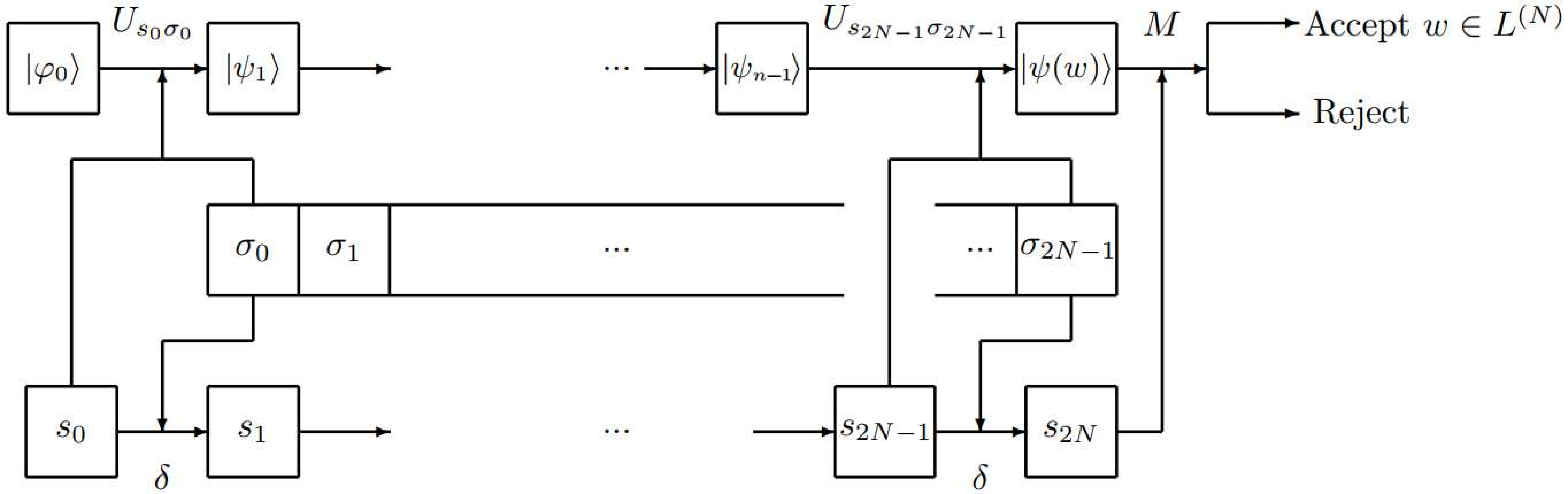
For PFA to recognize , we have:
Theorem 4.
For any , there exists a PFA with states recognizing , satisfying that the accepting probability for and for .
Proof.
Due to Theorem 10 by Ambainis and Freivalds in [21], there exists a PFA with states recognizing with probability , that is, and for . We construct a PFA recognizing with probability , where is an identity operator and the others are defined as follows:
- •
, and for convenience, we denote the states in as ;
- •
;
- •
, , ;
- •
, where represents a vector in that all of its elements are 1.
For any input string , works as follows. According to the definition of , if , then the resulting state of computing is , where and is a superposition state. Hence will be accepted with probability
If , then the state of is , where is a superposition state. Hence the accepting probability of is
If , that is , then we have
| (45) | ||||
| (46) | ||||
| (47) | ||||
| (48) | ||||
| (49) |
Hence, if , will be accepted with probability greater than , otherwise will be accepted with probability less than .
Remark 4.
So, for prefix-closured regular language , there exists a 1QFAC having classical states and quantum basis states to recognize with bounded error, and there exists a PFA with states recognizing with bounded error. However, we still do not know the lower bound on the state complexity of PFA for recognizing .
4.2 Supervisory Control of QDES simulated with cut-point languages
Let be a 1QFAC, and let () be the set of specifications we hope to achieve, where is also a regular language that is recognized by a 1QFAC with cut-point () isolated by . First, we give a sufficient condition such that there is a quantum supervisor controlling QDES to approximate to , and this is the first supervisory control theorem of QDES.
From now on, a QDES associated with a 1QFAC always has , that is, the initial state is an accepting state.
Theorem 5.
Let be a finite event set and . Suppose a QDES with event set is modeled as for a 1QFAC with . Let be recognized by a 1QFAC with cut-point () isolated by , where and (but for ). If , ,
| (50) |
then there is a quantum supervisor such that
| (51) |
Proof.
Let
| (52) |
Recall , ,
| (53) |
Suppose that for . Then ,
| (54) |
On the other hand,
| (55) | ||||
| (56) |
Remark 5.
Theorem 5 shows that under certain conditions, there is a quantum supervisor to achieve an approximate objective specification. Next we give a sufficient and necessary condition for the existence of quantum supervisor to achieve a precise supervisory control, and this is described by the following theorem.
Theorem 6.
Let be a finite event set and . Suppose a QDES with event set is modeled as a quantum language that is generated by an 1QFAC . Quantum language generated by some 1QFAC satisfies . Then there is a quantum supervisor such that , if and only if , ,
| (57) |
Proof.
). Let
| (58) |
First holds as we suppose the initial state is an accepting state. Recall , ,
| (59) |
Suppose that for . Then ,
| (60) |
On the other hand,
| (61) | ||||
| (62) | ||||
| (63) |
). Let quantum supervisor satisfy that for any , any .
| (64) | ||||
| (65) | ||||
| (66) | ||||
| (67) |
So, we complete the proof of theorem.
From Theorem 6 we can obtain a corollary, and this is a modelling fashion of QDES with cut-point.
Corollary 2.
Suppose a QDES is modeled as a cut-point language recognized by a 1QFAC with . Quantum language generated by some 1QFAC satisfies . Then there is a quantum supervisor such that , if and only if , , if , then .
4.3 An example to illustrate supervisory control theorems of QDES
Theorem 6 and its Corollary 2 are the main supervisory control results of QDES. As an application of Theorem 6 (or Corollary 2), we present an example to show the advantage of QDES over classical DES in state complexity.
Example 3.
We employ the language in Example 1. Let , , . Given an natural number , suppose a QDES modeled as the cut-point language
| (69) |
recognized by a 1QFAC with cut-point , and quantum language is generated by another 1QFAC that will be defined in the following.
is defined as Example 1, and for any iff .
For any given natural number , we consider the language that is recognized by another 1QFAC with cut-point . can be defined by means of , and for any iff .
Therefore, we have and .
It is immediate to check that the condition “, , if , then ” in Corollary 2 holds, so there is a quantum supervisor such that .
Due to Theorem 2, we know that PFA (i.e., PDES) require and states to recognize the languages and with cut-point , respectively. So, QDES show essential advantage over classical DES in state complexity for simulation of systems.
4.4 Supervisory Control of QDES simulated with isolated cut-point languages
In this section we study nonblocking problem in QDES. In this case, it is more suitsble to consider QDES simulated with the languages (say ) of cut-point isolated by an , and the controlled language by quantum supervisor is required to belong to this language . Our main purpose is to establish nonblocking quantum supervisor theorem in QDES.
First, we would recall nonblocking problem in classical DES [1, 2]. Let a DES modeled by finite automaton . Then is called nonblocking if . That is, for any feasible input string , input string will reach a marked state for some string . Let be a supervisor. Then the language marked by is defined as:
| (70) |
The DES modeled by is nonblocking if In practice, being nonblocking is important since it leads to each string in together with some more input string being able to reach a marked state.
Suppose that 1QFAC recognizes a language (denoted by ) over alphabet with cut-point isolated by . For any , denote
| (71) |
and
| (72) |
For any quantum language over , denote by the support set of , i.e., . A quantum supervisor is called as nonblocking if it satisfies .
Theorem 7.
Suppose a QDES is modeled as a language recognized by a 1QFAC with cut-point isolated by . is a quantum language over . Let . Then there is a quantum supervisor satisfying nonblocking (i.e., ) such that and if and only if
- 1.
, ,
(73) - 2.
,
(74)
Proof.
). , let
| (75) |
First, (). Suppose and , . Then ,
(I) if , then
| (76) | ||||
| (77) | ||||
| (78) | ||||
| (79) |
(II) if , then it holds as well, since . On the other hand,
| (80) | ||||
| (81) | ||||
| (82) |
So, .
For any , if , then ; if , then with condition 2) above, we have
| (83) | ||||
| (84) | ||||
| (85) | ||||
| (86) |
). 1) , , since quantum supervisor always satisfies that , we have
| (87) | ||||
| (88) | ||||
| (89) |
2) , if , then and ; if , then
| (90) | ||||
| (91) | ||||
| (92) |
Consequently, the proof is completed.
As a special case of Theorem 7, the following corollary follows.
Corollary 3.
Suppose a QDES is modeled as a language recognized by a 1QFAC with cut point isolated by . is a regular language. Let . Then there is a quantum supervisor satisfying such that and if and only if the following two conditions hold:
- 1.
(93) - 2.
(94)
where .
Proof.
In fact, we can do it by taking as a classical language in Theorem 7. So, we omit the details here.
5 Decidability of Controllability Condition
In supervisory control of QDES, the controllability conditions play an important role of the existence of quantum supervisors. So, we present a polynomial-time algorithm to decide the controllability condition Eq. (57). The prefix-closure of quantum language , as the target language we hope to achieve under the supervisory control, is in general generated by a 1QFAC , that is, . Then the controllability condition Eq. (57) is equivalently as: , ,
| (95) |
First, we need a proposition.
Proposition 5.
Suppose a QDES modeled as a quantum language that is generated by a 1QFAC . Quantum language satisfies , and for some 1QFAC . Then and for any , and .
Proof.
By the definition of prefix closure, for any , and , we have and , which result in .
Furthermore, due to and , we have , that is, for any , and , .
In the light of Proposition 5, we have:
| (96) | ||||
| (97) | ||||
| (98) | ||||
| (99) | ||||
| (100) | ||||
| (101) | ||||
| (102) | ||||
| (103) | ||||
| (104) |
So, Inequality (95) is equivalent to Eq. (104), and therefore it suffices to check whether Eq. (104) holds for any , and for each , in order to check the controllability condition.
In fact, we have the following result, where and are the numbers of quantum basis states of and , respectively.
Theorem 8.
Suppose a QDES modeled as a quantum language generated by a 1QFAC . For quantum language , is generated by another 1QFAC and . Then the controllability condition Eq. (57) holds if and only if for any , for any with , Eq. (95) holds. Furthermore, there exists a polynomial-time algorithm running in time that determines whether the controllability condition Eq. (57) holds.
Proof.
According to Lemma 1, 1QFAC and can be simulated by two RBLM, say and respectively, such that ,
| (105) |
| (106) |
and the numbers of states in and are and , respectively, where and represent respectively the numbers of classical states in and , and represent respectively the numbers of quantum states in and , and functions and are associated to and , respectively.
Similarly, by virtue of Proposition 2 and Lemma 1, for each , there exist two RBLM and respectively satisfying that ,
- 1.
(107) - 2.
(108)
where the numbers of states in and are also and , respectively. Therefore, ,
- 1.
(109) - 2.
(110) - 3.
(111) - 4.
(112)
where the second equalities of each equations above are due to Remark 1. Therefore, equation (104) is equivalent to
| (113) |
for every . Furthermore, by means of Remark 1, we have
| (114) |
for every , where the state numbers of and are the same as
| (115) | ||||
| (116) |
By virtue of Proposition 1, the above Equation (114) holds for every if and only if it holds for all with , and there exists a polynomial-time algorithm running in time to determine whether Equation (114) holds for every . Here we present the algorithm in detail, but omit the analyses of correctness and complexity and the details are referred to [35, 36, 40, 41, 42, 43].
In the first step, given 1QFAC and , and for any , we can directly construct two RBLM and as above, and for simplicity, we denote them respectively by
- •
,
- •
.
Recalling Definition 1 and Remark 1, we have
| (117) |
their direct sum is
| (118) | ||||
| (119) |
and then
| (120) |
for any . For any , denote
| (121) |
for
Now we present Algorithm 1 to check whether or not and are equivalent.
So, if for any , Algorithm 1 returns and are equivalent, then the controllability condition holds; otherwise the controllability condition does not hold.
6 Concluding Remarks
As a kind of important control systems, DES have been developed deeply [1]-[9] due to the potential of practical application, but state complexity is still a key problem in DES to be solved appropriately. In recent thirty years, quantum computing has been studied rapidly [11], and quantum control has attracted great interest [17]. So, initiating the study of QDES likely becomes a new subject of DES, and it is also motivated by two aspects: one is the simulation of DES in quantum systems by virtue of the principle of quantum computing; another is that QDES have advantages over classical DES for processing some problems in state complexity. This paper has been the first study for establishing QDES in light of QFA.
In this paper, we have established a basic framework of QDES, and the supervisory control of QDES has been studied. The main contributions are: (1) We have used 1QFAC to simulate QDES, and proved that MO-1QFA are not suitable for modeling QDES since we found MO-1QFA cannot recognize any prefix-closured language even with cut-point. (2) We have established a number of supervisory control theorems of QDES and proved the sufficient and necessary conditions of the existence of quantum supervisors. (3) We have constructed a number of examples to illustrate the supervisory control theorems and these examples have also showed the advantages of QDES over classical DES concerning state complexity. (4) We have given a polynomial-time algorithm to determine whether or not the controllability condition holds.
In subsequent study, we would like to consider controllability and observability problem of QDES under partial observation of events, and decentralized control of QDES with multi-supervisors under partial observation of events, as well as diagnosability of QDES. In particular, we would like to discover more practical examples to illustrate the advantages of QDES over classical DES in state complexity.
Acknowledgements
I thank Ligang Xiao for useful discussion and helpful construction concerning the examples of QFA recognizing prefix-closured languages. This work is supported in part by the National Natural Science Foundation of China (No. 61876195).
References
- [1] C. G. Cassandras, S. Lafortune, Introduction to Discrete Event Systems. Springer: New York, 2nd edition, 2008.
- [2] W. M. Wonham, K. Cai, Supervisory Control of Discrete-Event Systems. Cham, Switzerland: Springer, 2019.
- [3] R. J. Ramadge, W. M. Wonham,“Supervisory control of a class of discrete event processes,”SIAM Journal on Control and Optimization, vol. 25, no. 1, pp. 206–230, 1987.
- [4] V. V. Kornyak,“Classical and quantum discrete dynamical systems,” Physics of Particles and Nuclei, vol. 44, pp. 47–91, 2013.
- [5] F. Lin,“Supervisory control of stochastic discrete event systems,” in Book of Abstracts, SIAM Conference Control 1990’s, San Francisco, 1990.
- [6] M. Lawford, W. M. Wonham,“Supervisory control of probabilistic discrete event systems,” in Proceedings of the 36th Midwest Symposium on Circuits and Systems, Detroit, MI, USA, Aug. 1993, pp. 327–331.
- [7] V. Pantelic, S. Postma, M. Lawford,“Probabilistic supervisory control of probabilistic discrete event systems,”IEEE Transactions on Automatic Control, vol. 54, no. 8, pp. 2013–2018, 2009.
- [8] F. Lin, H. Ying,“Modeling and control of fuzzy discrete event systems,” IEEE Transactions on Systems, Man, and Cybernetics, Part B (Cybernetics), vol. 32, no. 4, pp. 408–415, 2002.
- [9] D. W. Qiu, “Supervisory control of fuzzy discrete event systems: a formal approach,” IEEE Transactions on Systems, Man, and Cybernetics, Part B (Cybernetics), vol. 35, no. 1, pp. 72–88, 2005.
- [10] W. Deng, J. Yang, D.W. Qiu, “Supervisory control of probabilistic discrete event systems under partial observation,” IEEE Transactions on Automatic Control, vol. 64, no. 12, pp. 5051–5065, 2019.
- [11] M.A. Nielsen, I.L. Chuang, Quantum Computation and Quantum Information. Cambridge University Press, Cambridge, 2000.
- [12] P. Benioff, “The computer as a physical system: a microscopic quantum mechanical Hamiltonian model of computers as represented by Turing machines,” Journal of Statistical Physics, vol. 22, pp. 563–591, 1980.
- [13] R. P. Feynman, “Simulting physics with computers,” International Journal of Theoretical Physics, vol. 21, pp. 467–488, 1982.
- [14] D. Deutsch, “Quantum theory, the Church-Turing principle and the universal quantum computer,” Proceedings of the Royal Society of London. Series A, vol. 400, no. 1818, pp. 97–117, 1985.
- [15] P. W. Shor, “Polynomial-time algorithms for prime factorization and discrete logarithms on a quantum computer,” SIAM Journal on Computing, vol. 26, no. 5, pp. 1484–1509, 1997.
- [16] H. I. Nurdina, M. R. James, I. R. Petersen, “Coherent quantum LQG control,” Automatica, vol. 45, pp. 1837–1846, 2009.
- [17] H. M. Wiseman, G. J. Milburn, Quantum Measurement and Control. Cambridge University Press, Cambridge, UK, 2010.
- [18] S. Lloyd,“Coherent quantum feedback,”Physical Review A, vol. 62, pp. 022108, 2000.
- [19] Richard J. Nelson, Y. Weinstein, D. Cory, S. Lloyd,“Experimental Demonstration of Fully Coherent Quantum Feedback,” Physical Review Letters, vol. 85, no. 14, pp. 3045-3048, 2000.
- [20] Y. Pencolé, M.-O. Cordier,“A formal framework for the decentralised diagnosis of large scale discrete event systems and its application to telecommunication networks,” Artificial Intelligence, vol. 164, pp. 121–170, 2005.
- [21] A. Ambainis, R. Freivalds,“One-way quantum finite automata: strengths, weaknesses and generalizations,” in:Proceedings of the 39th IEEE Symposium on Foundations of Computer Science, 1998, pp. 332–341.
- [22] A. Ambainis, A. Yakaryilmaz, “Automata and quantum computing,” in: Handbook of Automata Theory (II), pp. 1457-1493,2021. arXiv:1507.01988.
- [23] C. Mereghetti, B. Palano, S. Cialdi, et al., “Photonic Realization of a Quantum Finite Automaton,” Physical Review Research, vol. 2, 2020, Art. no. 013089.
- [24] S. Z. D. Plachta, M. Hiekkamäki, A. Yakaryilmaz, R. Fickler, “Quantum advantage using high-dimensional twisted photons as quantum finite automata,” Quantum, vol. 6, 752, 2022.
- [25] Y. Tian, T. Feng, M. Luo, S. Zheng, and X. Zhou, “Experimental demonstration of quantum finite automaton,” npj Quantum Information, vol.5, no. 1, pp. 1-5, 2019.
- [26] H. Nishimura and T. Yamakami, “An application of quantum finite automata to interactive proof systems,” Journal of Computer and System Sciences, vol. 75, no.4, pp. 255-269, 2009.
- [27] A.S. Bhatia and S. Zheng, “A quantum finite automata approach to modeling the chemical reactions,” Frontiers in Physics, vol. 8, 547370, 2020.
- [28] D. W. Qiu, L. Li, P. Mateus, J. Gruska, “Quantum Finite Automata,” in: J. Wang (Eds.), Finite State-Based Models and Applications, CRC Handbook, Boca Raton, pp. 113–144, 2012.
- [29] J. Gruska, Quantum Computing. McGraw-Hill, London, 1999.
- [30] A.S. Bhatia, A. Kumar, “Quantum finite automata: survey, status and research directions,” 2019, arXiv:1901.07992.
- [31] C. Moore, J. P. Crutchfield, “Quantum automata and quantum grammars,” Theoretical Computer Science, vol. 237, pp. 275–306, 2000.
- [32] A. Kondacs, J. Watrous, “On the power of finite state automata,” in Proceedings of the 38th IEEE Symposium on Foundations of Computer Science, 1997, pp. 66–75.
- [33] A. Brodsky, N. Pippenger, “Characterizations of 1-way quantum finite automata,” SIAM Journal on Computing, vol. 31, no. 5, pp. 1456–1478, 2002.
- [34] P. Mateus, D. W. Qiu, L. Li,“On the complexity of minimizing probabilistic and quantum automata,”Information and Computation, vol. 218, pp. 36–53, 2012.
- [35] D. W. Qiu, L. Li, X. Zou, P. Mateus, J. Gruska,“Multi-letter quantum finite automata: decidability of the equivalence and minimization of states,”Acta Informatica, vol. 48, pp. 271–290, 2011.
- [36] L. Z. Li, D. W. Qiu,“Determining the equivalence for one-way quantum finite automata,” Theoretical Computer Science, vol. 403, pp. 42–51, 2008.
- [37] D.W. Qiu, L. Li, P. Mateus, and A. Sernadas,“Exponentially more concise quantum recognition of non-RMM languages,”Journal of Computer and System Sciences, vol. 81, no. 2, pp. 359–375, 2015.
- [38] J. E. Hopcroft and J. D. Ullman, Introduction to Automata Theory, Languages, and Computation. Addison-Wesley, New York, 1979.
- [39] A. Paz, Introduction to Probabilistic Automata. Academic Press, New York, 1971.
- [40] C. Cortes, M. Mohri and A. Rastogi,“On the computation of some standard distances between probabilistic automata,” In: Proceedings of the 11th International Conference on Implementation and Application of Automata, 2006, pp. 137-149.
- [41] S. Kiefer, A.S. Murawski, J. Ouaknine, B. Wachter and J. Worrell, “Language equivalence for probabilistic automata,” In:Proceedings of the 23rd International Conference on Computer Aided Verification, 2011, pp. 526-540.
- [42] L. Li and Y. Feng, “Quantum Markov chains: description of hybrid systems, decidability of equivalence, and model checking linear-time properties,” Information and Computation, vol. 244, pp. 229-244, 2015.
- [43] Q. Wang, J. Liu and M. Ying,“Equivalence checking of quantum finite-state machines,” Journal of Computer and System Sciences, vol. 116, pp. 1-21, 2021.
- [44] D. Thorsley and D. Teneketzis,“Diagnosability of Stochastic Discrete-Event Systems,”IEEE Transactions on Automatic Control, vol. 50, no. 4, pp. 476-492, 2005.
- [45] C. Keroglou and C. N. Hadjicostis, “Detectability in stochastic discrete event systems”, Systems & Control Letters, vol. 84, pp. 21-26, 2015.
- [46] F. Liu and D. W. Qiu,“Safe diagnosability of stochastic discrete event systems,”IEEE Transactions on Automatic Control, vol. 53, no. 5, pp. 1291-1296, 2008.