Distribution-on-Distribution Regression via Optimal Transport Maps
Abstract
We present a framework for performing regression when both covariate and response are probability distributions on a compact interval. Our regression model is based on the theory of optimal transportation and links the conditional Fréchet mean of the response to the covariate via an optimal transport map. We define a Fréchet-least-squares estimator of this regression map, and establish its consistency and rate of convergence to the true map, under both full and partial observation of the regression pairs. Computation of the estimator is shown to reduce to a standard convex optimisation problem, and thus our regression model can be implemented with ease. We illustrate our methodology using real and simulated data.
Keywords:
Wasserstein metric,keywords
[class=AMS]keywords
and
1 Introduction
Functional data analysis [5] considers statistical inference problems whose sample and parameter spaces constitute function spaces. This framework encompasses data that are best viewed as realisations of random processes, and presents challenges arising from the infinite dimensionality of the function spaces, typically taken to be separable Hilbert spaces. On the other hand, non-Euclidean statistics [15] treats inference problems whose sample and parameter spaces are finite dimensional manifolds. Such problems present with a different set of challenges, linked with the non-linearity of the corresponding spaces, which often arises due to non-linear constraints satisfied by the data/parameters.
When the data/parameters of interest are, in fact, probability distributions, one has a problem that is simultaneously functional and non-Euclidean: on the one hand the data can be seen as random processes, and on the other they satisfy non-linear constraints, such as positivity and integral constraints. Thus, the functional data analysis of probability distributions features interesting challenges stemming from this dual nature of the ambient space, for example the finite measurement of intrinsically infinite dimensional objects, and the lack of a linear structure which is crucial to basic statistical operations, such as averaging or, more generally, regression toward a mean. See Petersen, Zhang and Kokozska 2021+ for an excellent overview.
One approach to dealing with the non-linear nature of probability distributions is to apply a suitable transformation and map the problem back to a space with a linear structure [6, 3, 16, 7]. A seemingly more natural approach is to embrace the intrinsic non-linearity, and to analyse the data in their native space, equipped with a canonical metric structure. In the case of probability distributions, the Wasserstein metric [13, 14] has been exhibited as a canonical choice [12], primarily because it captures deformations, which are typically the main form of variation for probability distributions.
The case of inferring the Fréchet mean of a collection of random elements in the Wasserstein space is by now well understood [12, 1, 21, 9]. The deep links to convexity and the tangent space structure of the Wasserstein space play an important role in motivating and deriving the analysis of this case. The next step is to understand the notion of regression of one probability distribution on another. The first to do so were Chen, Lin and Müller 2020, and, independently, Zhang, Kokoszka and Petersen 2020, the latter paper focussing on autoregression. They used the tangent space structure to define a regression operation: using the log transform, the regressor and response are lifted to suitable tangent spaces, where a (linear) regression model is defined in a more familiar Hilbertian setting [11, 4]. This allows the authors to use the well-developed toolbox of functional regression, and derive appropriate asymptotic theory.
In this paper, we propose an alternative notion of distribution-on-distribution regression, following a different path. Rather than taking a geometrical approach, via the tangent bundle structure, we follow a shape-constraint approach, namely exploiting convexity. Our model is defined directly at the level of the probability distributions, and stipulates that the response distributions are related to the covariate distributions by means of an optimal transport map, and further deformational noise. A key advantage of this approach is its clean and transparent interpretation, since the regression operator can be interpreted pointwise at the level of the original distributions, and its effect consists in mass transportation, or equivalently, quantile re-arrangement. Further to this, the approach requires minimal regularity conditions, and does not suffer from ill-posedness issues as inverse problems do. Finally, its computational implementation reduces to a standard convex optimisation problem. The usefulness of the approach is exhibited when revisiting the analysis of the mortality data of Chen, Lin and Müller 2020, where the approach is seen to lead to similar (if more expansive) qualitative conclusions, but with the advantage of an arguably improved interpretability.
2 Background on Optimal Transport and Some Notation
In order to define our regression model, we now provide some minimal background on optimal transport and Wasserstein distances, including some relevant notation. For more background see, e.g. [14]. Let and be the set of Borel probability measures on , with finite second moment. The 2-Wasserstein distance between is defined by
where is the set of couplings of and , i.e. the set of Borel probability measures on with marginals and . It can be shown that endowed with is a metric space, which we simply call the Wasserstein space of distributions. A coupling is deterministic if it is the joint distribution of for some deterministic map , called an optimal transport map. In such a case, we write and say that pushes forward to , i.e. for any Borel set . Occasionally we denote this as , for clarity.
When the source distribution is absolutely continuous with respect to the Lebesgue measure, then the optimal plan is induced by a map . When , the map admits the explicit expression , where is the quantile function of , and is the cumulative distribution function of . In addition
| (1) |
A notion of average of probability distributions can be defined via the Fréchet mean with respect to the Wasserstein metric. Namely, let be a random measure on with law . A Fréchet mean of is a minimizer of the Fréchet functional
The Fréchet functional can thus serve as a basis to define a sum-of-squares functional in the context of regression, and this will be done in the next section.
We will occasionally use the fact that is flat in that for it holds that
| (2) |
whenever the optimal maps involved are well-defined.
Finally, we will use the notation to indicate that there exists a positive constant for which holds. The support of a function will be denoted by . And, for a measure , we indicate the norm of a function with respect to as .
3 Distribution-on-Distribution Regression
3.1 Fréchet Functionals and Regression Operators
Let be a pair of random elements in with joint distribution . Then, similar to a standard nonparametric regression model, we can define a regression operator as the minimizer of the conditional Fréchet functional, viewed as a function of ,
assuming that for any , the Fréchet mean of the conditional law of given is unique , which can be enforced by means of regularity assumptions on the pair .
The difference between the above formulation and the standard regression formulation is that we have replaced the notion of expectation with a Wasserstein-Fréchet mean, an approach termed as “Fréchet Regression” by Petersen and Müller 2019. Postulating a specific form on the regression operator amounts to defining a certain type of regression model. If is left unconstrained, except for possessing some degree of regularity, then we would speak of a nonparametric regression model. However, assumptions on are needed to ensure its identifiability, and simply assuming it is regular will not suffice in this more general context.
For instance, the approach of Chen, Lin and Müller 2020 and Zhang, Kokoszka and Petersen 2020 consists in constraining to be in a certain sense linear, in that it can be represented as a linear operator at the level of the tangent bundle. Identifiability, and indeed fitting and asymptotic theory, can then be derived by appealing to the inclusion of the tangent spaces in Hilbert spaces.
Here we impose a different constraint on , and consequently define a different notion of regression. Namely we impose a shape constraint, by assuming that , where is an increasing map. This is developed in the next section which postulates a regression model on the pair that guarantees the uniqueness of the conditional Fréchet mean of given , and imposes mild conditions ensuring the identifiability of .
3.2 The Regression Model and The Fréchet-Least-Squares Estimator
Henceforth, we will take the domain to be a compact interval of . Let be an independent collection of regressor/response pairs in . Motivated by the discussion in the previous paragraph, we define the regression model
| (3) |
where is an unknown optimal map and is a collection of independent and identically distributed random optimal maps satisfying almost everywhere on . These represent the “noise” in our model. The regression task will be to estimate the unknown from the observations . To be able to do so, we need to ensure that is identifiable, and for this we now introduce some conditions.
In the spirit of Section 3.1, let be the probability law induced on by model (3). We denote by and the marginal distributions induced on the typical regressor and the typical response , respectively.
Assumption 3.1.
Let be a measure in the support of . Then is absolutely continuous with respect to Lebesgue measure on .
Denote by the measure that is linear average of , i.e. . We also denote by the empirical counterpart of , namely , where are independent random measures with law . Note that all in the support of are dominated by the measure , i.e. almost surely.
Define the parameter set of optimal transport maps as:
Implicit in the definition of is that its elements are assumed differentiable -a.e. In the presence of Assumption 3.1, the -a.e. existence of is automatically guaranteed, since Lebesgue’s theorem on the differentiation of monotone functions states that a monotone function automatically has a derivative Lebesgue almost everywhere in the interior of , and Assumption 3.1 implies that is dominated by Lebesgue measure.
We will also assume:
Assumption 3.2.
The model (3) is induced by a map and random maps that are of class .
With these assumptions in place, we can now establish identifiability:
Theorem 3.3.
Remark 3.4 (Identifiability -almost everywhere).
Theorem 3.3 establishes the identifiability of up to -null sets, with minimal assumptions on the input measures . Consequently, if the random covariate measure is almost surely supported on a strict subset , we can identify on (which coincides with the support of ) but not on . Of course, if the measure is equivalent to Lebesgue measure, in the sense of mutual absolute continuity, identifiablity will also hold Lebesgue almost everywhere on . Additional conditions on the law of the random covariate measure can yield this equivalence. A simple condition is to require , yielding that , where and are the Lebesgue densities of the measures and . However this condition implies that with positive probability, which can be restrictive as we would like our model to encompass situations where none of the covariate measures are fully supported on . A considerably weaker condition that guarantees the equivalence of to Lebesgue measure is to require the existence of a cover of such that for all – intuitively, this enables different covariate measures to give information on on different subsets of , but requires that they collectively provide information on all of . As an example let and let be defined as the normalised Lebesgue measure on , where is a uniform random variable on . In this case none of the realisations of are supported on , but the “cover condition” is satisfied.
Further to identifiability, the theorem gives a way to estimate by means of -estimation. We can define an estimator as the minimizer of the sample counterpart of ,
| (5) |
where are independent samples from for . In effect this a “Fréchet least square” estimator. The existence and uniqueness of a minimizer is not a priori obvious, but we establish both in the next section 3.4.
Remark 3.5 (Pure Intercept Model).
When all the input measures are equal, , our regression model reduces to a “pure intercept model”, which is equivalent to the problem of estimating a Fréchet mean. To see this, let a fixed measure. From the assumption that a.e., one can deduce that the conditional Fréchet mean of the measure , given the measure is equal to . Estimation of is then equivalent to estimation of the Fréchet mean of the output measures, since .
3.3 Interpretation and Comparison
It was argued in the introduction that the proposed regression model has the advantage of being easily interpretable, and now we elaborate on this point. The fact that the regressor operator takes the form
| (6) |
where is a monotone map, has a simple interpretation in terms of mass transport: the effect of the Fréchet mean in this regression is to transport the probability mass assigned by on a subinterval onto the transformed subinterval . Therefore, the model can be directly interpreted at the level of the quantity that the input/output measures are modelling. In particular, the model can be interpreted at the level of quantiles. Since
we can see that the mean effect of the regression is to move the -quantile of , say , to the new location . Each response distribution will then further deviate from its conditional Fréchet mean by means of a random monotone “error” map whose expectation is the identity map,
This highlights the analogy with a classical regression setup, except that the addition operation is replaced by the composition operation at the level of quantiles, or equivalently, by the push-forward operation at the level of distributions. In particular, the assumption that is directly analogous to the classical assumption that the errors have zero mean: one can directly see that for almost all implies that
Assuming that we have obtained an estimator of the regression map based on regressor/response pairs, we can then define the fitted distributions,
We can also define the th residual map as the optimal transport map that pushes forward the observed response to the fitted value . The residual maps can be plotted in a “residual plot” and contrasted to the identity map, by analogy to the classical regression case. This can help identify outlying observations, and also to appreciate in what manner the fitted values differ from the observe values. In particular, it can reveal in which regions of the support of the measures the model provides a good fit, and where less so. It can also serve to identify clusters of observations whose residuals are similar, suggesting the potential presence of a latent indicator variable, i.e. that separate regressions ought to be fit to different groups of observations. Finally, the residual plot can serve as a diagnostic tool for the validity of the model. Since the residual map can be seen as a proxy for the latent error map , deviations of the average of the residual maps from the identity can serve as a means to diagnose departures from the assumed model. Note that, contrary to classical regression, where the residuals sum to zero by construction, the residual maps are not constrained to have mean equal to the identity.
By comparison, Chen, Lin and Müller 2020 introduce (linear) regression in Wasserstein space by means of a geometric approach, that is in a sense a linear model between tangent spaces. Namely, for and , the Fréchet means of the regressor and response measures, they postulate a regressor operator of the form
| (7) |
where is the identity map on , and is a bounded linear operator with some assumptions, so that the terms involved be well-defined. Again, linearity guarantees identifiability. The expression appears convoluted, but the geometrical interpretation is simple: represents the image of under the log map at (see Section 2.3 of Panaretos and Zemel 2020). Equivalently, is the lifting of to the tangent space at . Once the regressor is lifted onto , the action of the regression operator is to map it to its image in via the bounded linear operator , as in a standard functional linear model. The final step is to push forward by this image plus the identity, i.e. , which retracts back onto and yields a measure (if is a monotone map, then this is equivalent to exponentiation, see Section 2.3 of Panaretos and Zemel 2020). The model is most easily interpretable on the tangent space, where it states that the expected lifting of the response at is related to the lifting of the regressor at by means of the linear operator . Similarly, fitted values are defined on the tangent space, and then can be retracted by the same push-forward operation.
The two approaches do not directly compare, and neither captures the other as a special case. Similarly, there is no reason to a priori expect that one model would typically outperform the other in terms of fit, and one can expect this to depend on the specific data set at hand. Thus, our method should be seen as an alternative rather than an attempt at an improved or more general version of regression. An apparent advantage of the regressor function (6), however, is an arguably easier and more direct interpretation of the regression effect, directly at the level regressor/response, through a monotone re-arrangement of probability mass, as discussed above. Indeed this allows a direct point-wise interpretation of the regression effect. The regressor (7) on the other hand allows for a traditional (functional) regression interpretation via the linear operator , albeit acting on the logarithms of regressor/response, which makes it harder to interpret the regression effect at the level of the original measures, since there are two transformations involved, one non-linear and one linear. Similar points can be made with regards to the residuals and residual plots. Another potential advantage is at the level of regularity conditions imposed on for the purposes of theory. Equation (7) leads to an inverse problem on the tangent space, as is standard with functional linear models, and thus requires more delicate technical assumptions on the problem, in addition to regularisation. By contrast, the shape-constrained approach (6) only requires monotonicity on the regressor . It also avoids the instabilities of an inverse problem.
The utility of our model illustrated in Section 5, which considers an example where the age-at-death distribution for country in 2013 serves as a response distribution, and the age-at-death distribution of the same country in 1983 serves as the regressor. Interestingly, it leads to similar fits and qualitative conclusions as the analysis of the same data by Chen, Lin and Müller 2020, while exhibiting a clean and more expansive interpretation. Indeed, our definition of residual maps help identify effects related to changes in infant mortality not easily detectable when looking only at the fitted distributions, and to identify an interesting clustering of observations. See Section 5 for more details.
3.4 Existence and Uniqueness of the Estimator
In this section, we establish the existence and uniqueness of the estimator . To show the existence, we use a variant of the Weierstrass theorem, namely Kurdila and Zabarankin 2006, stated for convenience as Theorem 6.1 in the Appendix. This requires establishing the convexity and Gateaux differentiability of the functional , and this we do in the next lemma:
Lemma 3.6 (Strict Convexity and Differentiability).
Let be the parameter set and suppose we have independent observations that are realizations of . Both the empirical functional and the population functional are strictly convex with respect to . Moreover the functionals and are Gateaux-differentiable on the set of optimal maps in with respect to the and distances, respectively. The corresponding derivatives of in the direction is:
| (8) |
and the derivative of in the direction is
| (9) |
where is the optimal map from to .
Since is a convex, closed, and bounded subset of functions, we may now apply the Weierstrass theorem cited above to conclude:
Proposition 3.7 (Existence and Uniqueness of the Estimator).
There exists a unique solution to the Fréchet sum-of-squares minimization problem (5), with uniqueness being in the sense.
3.5 Computation
Since the domain is one-dimensional, we have that
Furthermore, since the regressors are assumed absolutely continuous (Assumption 3.1), we can always write for an optimal map . We can therefore manipulate the Fréchet sum-of-squares and use a Riemann approximation to write
| (10) |
for user-defined nodes in an interval partition of , and . Writing and , we reduce the above approximate minimization of the Fréchet sum-of-squares to the solution of the following convex optimization problem:
| (11) |
where . The above problem resembles an isotonic regression problem with repeated measurements, and can be solved via the Pool-Adjacent-Violater-Algorithm (PAVA) [10].
3.6 Consistency and Rate of Convergence
In this section, we establish the asymptotic properties of the proposed estimators both in the case of the fully observed set of measures and the case where one only indirectly observes input/output distributions through i.i.d. samples from each. A natural risk function to measure the quality of the estimator is the Fréchet mean squared error:
Using the equation (2) we can rewrite the above risk as follows:
Thus, we can obtain consistency and convergence rates in Fréchet mean squared error using the criterion , in particular:
Theorem 3.8.
In many practical applications, one does not have not access to the measures . Instead, one has to make do with observing random samples from each and . In this case, a standard approach is to use smoothed proxies in lieu of the unobservable measures, usually assuming some more regularity. Let and be consistent estimators of and obtained from smoothing a random sample of size from each respective measure. Given such estimators, define a new estimator of as
| (13) |
where
Note that here one can use any estimators of and which are consistent in Wasserstein distance, provided is absolutely continuous. Then, the rate of convergence of will depend on the rate of convergence of and to and , respectively in the Wasserstein distance:
Theorem 3.9.
Precise values of can be obtained by choosing specific estimators and imposing additional regularity on the underlying regressor/response measures. For instance, one can follow the estimation approach of [20] and obtain the minimax rate of convergence over measures with densities in Besov classes.
Remark 3.10.
Note that can be any finite constant, however large. Its precise value does not influence the rate (14) itself, but only the constants. It is therefore not to be interpreted as a regularisation parameter. To be strictly faithful to the assumptions of Theorem 3.9, the computation could incorporate additional constraints of the form , as a discretization of . From a practical point of view, though, we always have , since is monotone. So maintaining the original formulation of Section 3.5 implicitly corresponds to some in Theorem 3.9 (recall that is the user-defined number of nodes in the Riemann sum approximation (10)).
4 Simulated Examples
In this section we illustrate the estimation framework and finite sample performance of the method by means of some simulations. First we generate random predictors . We consider random distributions that are mixtures of three independent Beta components. We choose the parameters of the Beta distributions to be uniformly distributed random variables on , with densities
The are arbitrary fixed mixture weights in , such that . As for the noise maps , we use the class of random optimal maps introduced in Panaretos and Zemel 2016. Let be an integer and define by
These are strictly increasing smooth functions satisfying and for any . These maps can be made random by replacing by an integer-valued random variable . If the distribution of is symmetric around zero, then it is straightforward to see that , for all , as required in the definition of model (3). We generate a discrete family of random maps by the following procedure, which is slightly different from the mixture family of maps introduced in [12]: for let be i.i.d. integer-valued symmetric random variables, and be the order statistics of i.i.d. uniform random variables on , independent of . The random maps are then defined as
where is defined as the ratio
As for the optimal map constituting the regression operator, we set . After having generated the random and , we generate the response distributions according to model (3), i.e. . Figure (1) depicts representative sample pairs of predictor and response densities.


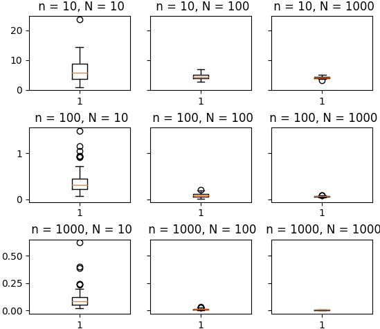
For estimation, we consider the case where we only observe independent samples from each pair of distributions . For simplicity, we use kernel density estimation, rather than the estimators in [20], to obtain the proxies and for the distributions and . Subsequently, for each , we estimate , where is the optimal map such that and solve the convex optimisation problem described in Section 3.5 to obtain the estimator . Figure (2) contrasts the estimated and true regression maps in each replication, for all nine combinations and . It is apparent that the dominant source of error is the bias due to partial observation, i.e. due to observing the measures through finite samples of size . When is moderately large (e.g. ) we see that the agreement between estimated and true map is very good, even for small values of . To quantitatively summarise the behaviour of the mean squared error in , we construct boxplots for the error in Figure (3), each based on 100 replications for the corresponding combination of and . The scale used is the same for each value of , in order to focus the behaviour with respect to .
5 Analysis of Mortality Data
We consider the age-at-death distributions for countries in the years 1983 and 2013, obtained from the Human Mortality Database of UC Berkeley and the Max Planck Institute for Demographic Research, openly accessible on www.mortality.org. Death rates are provided by single years of age up to 109, with an open age interval for 110+. We use Gaussian kernel density smoothing, to obtain age-at-death densities from the count data. Denote by the age-at-death distribution for the th country at year 1983 and the age-at-death distribution for the same country at year 2013. We use the distributions and as predictor and response distributions respectively. We chose these two years to allow comparison with Chen, Lin and Müller 2020, who illustrate their methodology on the same data set, and same pair of years.


We fit the model (3) by means of the approach described in Section 3.5 to obtain the estimated regression map based on the countries. This is depicted in Figure 4. The map dominates the identity map pointwise, indicating that the regression effect is to transport the mass of the age-at-death distribution to the right at visually all locations. Said differently, the map indicates an effect of net improvement in mortality across all ages. The most pronounced such effect is observed in young ages (between 0-10), where the regression map rises steeply: The proportion of the population dying at ages 0-10 in 1983 is redistributed approximately over the range 0-30 in 2013. The form of the map restricted to is approximately linear, indicating that this redistribution is achieved by conserving the actual shape of the distribution but scaling by a constant. The effect is still visible though less pronounced in the early adult to middle age range: The proportion of the population dying at ages between 20 and 60 in 1983 is approximately redistributed over ages 40-60 in 2013. The regression map is approximately parallel to the identity map on the range 60-80, shifted upwards by about 10 years indicating a translation of that interval by that amount of years between 1983 and 2013, i.e. the proportion of the population dying between 60-80 in 1983 has shifted to ages 70-90, but the shape of the distribution of that proportion over each of these two 20 year periods is approximately conserved. Overall, the regression map approximately resembles a piecewise linear map, allowing to interpret it locally by translations and dilations.


It is not easy to directly compare the effects expressed via this estimated regression map with the effects reflected by the estimated regression coefficient function , that is, the integral kernel of the operator in Equation (7) obtained in Chen, Lin and Müller 2020, when fitting their model to the same data. This is largely due to fact that the acts on tangent space elements, and thus is rather subtle to interpret. In interpreting their estimated regression operator, those authors remarked that the estimated was stratified according to the argument so that, “if the log-transformed predictor is non-negative or non-positive throughout its domain, then the fit for the log-transformed response is determined by the comparison of the absolute values of the log transformed predictor over the positive and negative strata of the estimated coefficient ”.
Using the estimated map we can then compute the fitted age-at-death distributions for the year 2013, namely . Figure (6) depicts the predictor and response densities as well as fitted response densities for a sample of 8 different countries. The first four of these countries (Japan, Ukraine, Italy and USA) were also selected as representative examples in Chen, Lin and Müller 2020. All eight countries exhibit a negatively-skewed age-at-death distribution. Comparing the actual distributions for the years 1983 and 2013 we can observe the decreasing trend in infant death counts and peaks shifting to older ages, as dictated by the fitted regression map. Contrasting observed and fitted distributions for 2013 allows for better comparison with the model output in [2], than does comparing the estimated regression operators.
Indeed, the main observations made in [2] are also apparent from our fitted model. In the case of our model, besides looking at the shape of the predicted densities, we can also take advantage of the direct interpretability of the residual maps , where is the optimal map between the fitted response and actual response . The collection of residual maps is plotted in Figure (7). It is apparent that the pointwise variability declines for progressively older ages, illustrating that it is harder to fit mortality at younger ages. One can then focus on the residual maps of specific countries. For example, doing so in the case of Japan and Ukraine, we reproduce the observation in [2] that “for Japan, the rightward mortality shift is seen to be more expressed than suggested by the fitted model, so that longevity extension is more than is anticipated, while the mortality distribution for Ukraine seems to shift to the right at a slower pace than the fitted model would suggest”. Similarly, we recover the same inference as in [2] regarding the US: “while the evolution of the mortality distributions for Japan and Ukraine can be viewed as mainly a rightward shift over calendar years, this is not the case for USA, where compared with the fitted response, the actual rightward shift of the mortality distribution seems to be accelerated for those above age 75 [note: 65 in our case], and decelerated for those below age 70 [note: 65 in our case]”. In terms of fit as measured by the Wasserstein distance between response and fit, both models have a harder time fitting Japan, ours doing slightly worse. On the flip side, our model fits Italy better, and the US and Ukraine considerably better (we only contrast countries explicitly mentioned in [2]).
Figure 5 features the overlay of all residual maps, in order to explore the goodness-of-fit of the model as well as the validity of the model assumptions. As the figure shows, the mean of residuals almost matches the identity map, which provides evidence in support of our model specification, in that the residual effects after correcting for the regression should have mean identity, reflected by the assumption that . Note that, contrary to usual least squares where the residuals have empirical mean zero, the residual maps need not have mean identity exactly.


Finally, we can scrutinise the individual residual maps for each of the 37 countries which we plot separately in Figures (8(a)) and (8(b)). The separation into two figures is deliberate, and is based on an apparent clustering: in Figure (8(a)) one can observe more of a rightward shift of fitted mortalities compared to the observed moralities for the countries concerned. This contrasts to countries in Figure (8(b)) which feature less of a rightward shift than fitted by the model. In a sense, these are clusters of “underfitted” and “overfitted” observations. Interestingly countries in Figure (8(a)) belong mostly to Eastern Europe plus Portugal, Spain, Italy, Israel, Japan and Taiwan. Countries in figure (8(b)) belong to western/northern European countries plus USA, New Zealand and Australia. Thanks to the pointwise interpretability of the residual maps, one can notice a particular contrast between these two groups of countries in terms of their fitted/observed infant mortality rates. This may be related to the fact that countries in Figure (8(a)) experienced a more pronounced improvement in their health care systems over the period 1983-2013, compared countries in Figure (8(b)) where healthcare was of comparably high quality already in 1983. It is interesting to note that Japan and Taiwan feature residual maps that everywhere dominate the identity.
6 Proofs
Proof of Lemma 3.6.
Using the closed form of optimal transport maps when , one can write:
The expression above shows that is convex with respect to since the map is convex and also integration preserves convexity. To show the strict convexity we should prove that for all and all such that ,
In fact by expanding the squares in the equality and doing some algebra one can conclude that the equality happens if and only if . Thus , and similarly , are strictly convex.
Notice that the domain of definition of can be extended to the space of functions. Therefore the Gateaux derivative of in the direction of can be defined as:
Expanding the first term we have:
| (15) |
The last equality is true since
Since , we can conclude
where is the optimal map from to . One can use a similar argument to derive the derivative of .
∎
Proof of Theorem 3.3.
We prove that is the unique minimizer of the population functional in . Suppose for some fixed measure , where by assumption almost everywhere. Thus according to Proposition 3.2.11 of [14], is the Fréchet mean of the conditional probability law of given or equivalently, for any
where is the joint distribution of induced by Model (3). Now is a minimizer of the above functional, since for any :
Also since is strictly convex w.r.t. , and integration preserves strict convexity, the functional is strictly convex. So is, in fact, the unique minimizer. ∎
To establish Proposition 3.7, we will use the following theorem.
Theorem 6.1 (Kurdila and Zabarankin 2006, Theorem 7.3.6).
Let be a reflexive Banach space and suppose that is Gateaux-differentiable on the closed, convex and bounded subset . If any of the following three conditions holds true,
- 1.
is convex over ,
- 2.
is monotone over ,
- 3.
is positive over ,
then all three conditions hold, and there exists an such that
Proof of Proposition 3.7.
To establish the consistency and rate of convergence of our estimator, we will make use of the theory of -estimation. To this aim, we restate some key theorems from Van Der Vaart and Wellner 1996.
Theorem 6.2 (Van Der Vaart and Wellner 1996, Theorem 3.2.3).
Let be random functions for positive integer , and let be a fixed function of such that for any
| (16) |
| (17) |
Then any sequence of estimators with converges in probability to .
Theorem 6.3 (Van Der Vaart and Wellner 1996, Theorem 3.2.5).
Let be a stochastic process indexed by a metric space , and let be a deterministic function, such that for every in a neighborhood of ,
Suppose that, for every and sufficiently small ,
for functions such that is decreasing for some (not depending on ). Let
If the sequence satisfies , and converges in outer probability to , then . If the displayed conditions are valid for every and , then the condition that is consistent is unnecessary.
Theorem 6.4 (Van Der Vaart and Wellner 1996, Theorem 2.7.5).
The class of monotone functions satisfies
for every probability measure , every , and a constant that depends only on .
Theorem 6.5 (Van Der Vaart and Wellner 1996, Theorem 3.4.2).
Let be class of measurable functions such that and for every in . Then
where .
Proof of Theorem 3.8.
Recall that, from Lemma 3.7, is the minimizer of the following criterion within the function class :
And the “true” optimal map is the minimizer of the following criterion function,
First we obtain an adequate upper bound for the bracketing number of the class of functions indexed by of the form:
where the domain of each function is . Denote by the bracketing entropy of the function class . One can directly control this bracketing entropy by the bracketing entropy of the class of optimal maps since
| (18) |
Since optimal maps are monotone functions, using Lemma 6.4, we know , and thus we conclude
The first line of the inequality (18) also shows that
for all .
To get the rate of convergence, we first show that has quadratic growth around its minimizer. For any map , we can write , where . Thus the equation (15), with and also the fact yields
Next, we find a function such that
Since the functions in are uniformly bounded and for all , the conditions of Theorem 6.5 are satisfied and we can choose
where the constant is a uniform upper bound for the functions in class . Since we noted that for any , we can show
The above inequality and the required condition gives the bound .
∎
To establish the rate of convergence under imperfect observation we will make use of the following Lemma.
Lemma 6.6.
Let be a sequence of measures converging in Wasserstein distance to a measure at a rate of convergence and let . Then .
Proof.
For simplicity and without loss of generality assume that exactly. If is the optimal map from to , then
Since is differentiable almost everywhere, and satisfies for almost all , then is Lipschitz continuous with Lipschitz constant at most . Thus
| (19) |
∎
Proof of Theorem 3.9.
Define . For any map ,
| (20) |
where , and is the rate of estimation of an absolutely continuous measure from samples. Thus the above inequality shows the uniform convergence of to (at a rate independent of ). Also, since is the unique minimizer of , according to Theorem 6.2, is a consistent estimator for , when is fixed.
Now assuming is fixed, we again use Theorem 6.3 for functionals and . Since both functionals are differentiable, the first condition of the Theorem (quadratic growth) is satisfied. For the second condition we need to find an upper bound for
| (21) |
According to (20), we have We also need , thus . Therefore
and
thus
∎
| Country List Figure (8(a)) | |
|---|---|
| Country Name | Country Code |
| Estonia | EST |
| Slovakia | SVK |
| Bulgaria | BGR |
| Hungary | HUN |
| Czechia | CZE |
| Lithuania | LTU |
| East Germany | DEUTE |
| Latvia | LVA |
| Belarus | BLR |
| Ukraine | UKR |
| Israel | ISR |
| Slovenia | SVN |
| Poland | POL |
| Spain | ESP |
| Italy | ITA |
| Portugal | PRT |
| Russia | RUS |
| Japan | JPN |
| Taiwan | TWN |
| Greece | GRC |
| Country List Figure (8(b)) | |
|---|---|
| Country Name | Country Code |
| Australia | AUS |
| West Germany | DEUTW |
| Austria | AUT |
| Netherlands | NLD |
| Iceland | ISL |
| Ireland | IRL |
| Belgium | BEL |
| France | FRATNP |
| Finland | FIN |
| New Zealand | NZL-NP |
| Switzerland | CHE |
| Sweden | SWE |
| Norway | NOR |
| United Kingdom | GBR-NP |
| U.S.A. | USA |
| Denmark | DNK |
| Luxemburg | LUX |
References
- Bigot et al. [2018] [author] Bigot, JérémieJ., Gouet, RaúlR., Klein, ThierryT., Lopez, AlfredoA. et al. (2018). Upper and lower risk bounds for estimating the Wasserstein barycenter of random measures on the real line. Electronic journal of statistics 12 2253–2289. \endbibitem
- Chen, Lin and Müller [2020] [author] Chen, YaqingY., Lin, ZhenhuaZ. and Müller, Hans-GeorgH.-G. (2020). Wasserstein regression. arXiv preprint arXiv:2006.09660. \endbibitem
- Delicado [2011] [author] Delicado, PedroP. (2011). Dimensionality reduction when data are density functions. Computational Statistics & Data Analysis 55 401–420. \endbibitem
- Hall et al. [2007] [author] Hall, PeterP., Horowitz, Joel LJ. L. et al. (2007). Methodology and convergence rates for functional linear regression. Annals of Statistics 35 70–91. \endbibitem
- Hsing and Eubank [2015] [author] Hsing, TailenT. and Eubank, RandallR. (2015). Theoretical foundations of functional data analysis, with an introduction to linear operators 997. John Wiley & Sons. \endbibitem
- Kneip and Utikal [2001] [author] Kneip, AloisA. and Utikal, Klaus JK. J. (2001). Inference for density families using functional principal component analysis. Journal of the American Statistical Association 96 519–542. \endbibitem
- Kokoszka et al. [2019] [author] Kokoszka, PiotrP., Miao, HongH., Petersen, AlexanderA. and Shang, Han LinH. L. (2019). Forecasting of density functions with an application to cross-sectional and intraday returns. International Journal of Forecasting 35 1304–1317. \endbibitem
- Kurdila and Zabarankin [2006] [author] Kurdila, Andrew JA. J. and Zabarankin, MichaelM. (2006). Convex functional analysis. Springer Science & Business Media. \endbibitem
- Le Gouic et al. [2019] [author] Le Gouic, ThibautT., Paris, QuentinQ., Rigollet, PhilippeP. and Stromme, Austin JA. J. (2019). Fast convergence of empirical barycenters in Alexandrov spaces and the Wasserstein space. arXiv preprint arXiv:1908.00828. \endbibitem
- Mair, Hornik and de Leeuw [2009] [author] Mair, PatrickP., Hornik, KurtK. and de Leeuw, JanJ. (2009). Isotone optimization in R: pool-adjacent-violators algorithm (PAVA) and active set methods. Journal of statistical software 32 1–24. \endbibitem
- Morris [2015] [author] Morris, Jeffrey SJ. S. (2015). Functional regression. Annual Review of Statistics and Its Application 2 321–359. \endbibitem
- Panaretos and Zemel [2016] [author] Panaretos, Victor MV. M. and Zemel, YoavY. (2016). Amplitude and phase variation of point processes. The Annals of Statistics 44 771–812. \endbibitem
- Panaretos and Zemel [2019] [author] Panaretos, Victor MV. M. and Zemel, YoavY. (2019). Statistical aspects of Wasserstein distances. Annual review of statistics and its application 6 405–431. \endbibitem
- Panaretos and Zemel [2020] [author] Panaretos, Victor MV. M. and Zemel, YoavY. (2020). An invitation to statistics in Wasserstein space. Springer Nature. \endbibitem
- Patrangenaru and Ellingson [2015] [author] Patrangenaru, VictorV. and Ellingson, LeifL. (2015). Nonparametric statistics on manifolds and their applications to object data analysis. CRC Press. \endbibitem
- Petersen et al. [2016] [author] Petersen, AlexanderA., Müller, Hans-GeorgH.-G. et al. (2016). Functional data analysis for density functions by transformation to a Hilbert space. Annals of Statistics 44 183–218. \endbibitem
- Petersen and Müller [2019] [author] Petersen, AlexanderA. and Müller, Hans-GeorgH.-G. (2019). Fréchet regression for random objects with Euclidean predictors. Annals of Statistics 47 691–719. \endbibitem
- Petersen, Zhang and Kokozska [2021+] [author] Petersen, AlexanderA., Zhang, ChaoC. and Kokozska, PiotrP. (2021+). Modeling Probability Density Functions as Data Objects. Econometrics and Statistics (to appear). \endbibitem
- Van Der Vaart and Wellner [1996] [author] Van Der Vaart, Aad WA. W. and Wellner, Jon AJ. A. (1996). Weak convergence. In Weak convergence and empirical processes 16–28. Springer. \endbibitem
- Weed and Berthet [2019] [author] Weed, JonathanJ. and Berthet, QuentinQ. (2019). Estimation of smooth densities in Wasserstein distance. arXiv preprint arXiv:1902.01778. \endbibitem
- Zemel and Panaretos [2019] [author] Zemel, YoavY. and Panaretos, Victor M.V. M. (2019). Fréchet means and Procrustes analysis in Wasserstein space. Bernoulli 25 932–976. \endbibitem
- Zhang, Kokoszka and Petersen [2020] [author] Zhang, ChaoC., Kokoszka, PiotrP. and Petersen, AlexanderA. (2020). Wasserstein Autoregressive Models for Density Time Series. arXiv preprint arXiv:2006.12640. \endbibitem