1Introduction

Cubic Action in Double Field Theory

Chen-Te Ma^a,b,c,d,e ¹¹ 1 e-mail address: yefgst@gmail.com

^a Guangdong Provincial Key Laboratory of Nuclear Science,
Institute of Quantum Matter, South China Normal University, Guangzhou 510006, Guangdong, China.
^b School of Physics and Telecommunication Engineering,
South China Normal University, Guangzhou 510006, Guangdong, China.
^c Guangdong-Hong Kong Joint Laboratory of Quantum Matter,
Southern Nuclear Science Computing Center, South China Normal University, Guangzhou 510006, Guangdong, China.
^d The Laboratory for Quantum Gravity and Strings,
Department of Mathematics and Applied Mathematics, University of Cape Town, Private Bag, Rondebosch 7700, South Africa.
^e Department of Physics and Center for Theoretical Sciences,
National Taiwan University, Taipei 10617, Taiwan, R.O.C.

We study target space theory on a torus for the states with $N_{L}+N_{R}=2$ through Double Field Theory. The spin-two Fierz-Pauli fields are not allowed when all spatial dimensions are non-compact. The massive states provide both non-vanishing momentum and winding numbers in the target space theory. To derive the cubic action, we provide the unique constraint for $N_{L}\neq N_{R}$ compatible with the integration by part. We first make a correspondence of massive and massless fields. The quadratic action is gauge invariant by introducing the mass term. We then proceed to the cubic order. The cubic action is also gauge invariant by introducing the coupling between the one-form field and other fields. The massive states do not follow the consistent truncation. One should expect the self-consistent theory by summing over infinite modes. Hence the naive expectation is wrong up to the cubic order. In the end, we show that the momentum and winding modes cannot both appear for only one compact doubled space.

1 Introduction

String Theory describes the dynamics of a one-dimensional object. When a distance scale is much larger than the string scale, a string behaves like a point particle. The oscillation of a string generates the graviton and other fields. Because String Theory is ultraviolet (UV) complete, it is a candidate to provide a consistent Quantum Gravity.

String Theory compactified on a $d$ -dimensional torus $T^{d}$ has a peculiar O( $d$ , $d$ ; $\mathbb{Z}$ ) symmetry [1, 2]. Indeed, strings can propagate along and wrap non-contractible cycles in spacetime. It generates winding states that have no analogue for particle theories. Hence one can claim that O( $d$ , $d$ ; $\mathbb{Z}$ ) symmetry is stringy. For a rectangular torus, the momentum number $n_{a}$ is related to the momentum $p_{a}$ along the circle of radius $R_{a}$ by the following definition:

\displaystyle p_{a}\equiv\frac{n_{a}}{R_{a}};\qquad n_{a}\in\mathbf{Z};\qquad a=1,2,\cdots,d;

(1)

where $R_{a}$ is radius of a circle. The number of times the string winds around a circle is instead the winding number $m_{a}$ , associated with the winding $\omega_{a}$ through:

\displaystyle\omega_{a}\equiv m_{a}\frac{R_{a}}{\alpha^{\prime}};\qquad m_{a}\in\mathbf{Z},

(2)

where $\alpha^{\prime}$ is the Regge slope parameter. The characterization of spectrum in the non-compact Minkowski spacetime is by the following squared of mass:

\displaystyle{\cal M}^{2}\equiv-k^{2}=p^{2}+\omega^{2}+\frac{2}{\alpha^{\prime}}(N_{L}+N_{R}-2),

(3)

where the momenta along the non-compact directions are $k^{\mu}$ while $N_{L}$ and $N_{R}$ are the numbers of left- and right-moving oscillators. We label the non-compact directions by $\mu=0,1,\cdots,25-d$ . The spectrum is invariant under the target-space duality (T-duality) [3, 4]. Under the T-duality, exchanging $n_{a}$ and $m_{a}$ together with the exchange of $R_{a}$ and $\alpha^{\prime}/R_{a}$ [3, 4]. Introducing simultaneously the coordinates $X^{a}$ for $T^{d}$ together with their duals $\tilde{X}_{a}$ can provide T-duality to a manifest symmetry. This symmetric structure provides the manifest T-dual invariant formulation of the first-quantized String Theory [5, 6, 7, 8] and its target space [7, 9].

The closed string field theory (second-quantized String Theory) [10, 11, 12, 13, 14] on a doubled torus naturally exhibits a manifest T-duality structure. The manifest structure keeps the momentum and winding modes simultaneously. Therefore, it inspires Double Field Theory [15]. When restricting to half degrees of freedom, Double Field Theory reveals to be based on Generalized Geometry [16, 17]. The tangent space at each point of the target space becomes a direct sum of the tangent and cotangent spaces.

The on-shell string states have to satisfy the level matching condition

\displaystyle L_{0}=\bar{L}_{0}

(4)

and the free string on-shell condition. The $L_{0}$ and $\bar{L}_{0}$ are Virasoro operators. The free string on-shell condition determines the spectrum. When all the dimensions of the target space are uncompactified in the bosonic string theory, the level matching condition implies that

\displaystyle N_{L}=N_{R},

(5)

where $N_{L}$ ( $N_{R}$ ) is the number of left (right)-moving oscillators.

In particular, massless states in the spectrum require $(N_{L},N_{R})=(1,1)$ . Therefore, the level matching condition gives a restriction. In the presence, instead, of compact dimensions in the target space, one obtains

\displaystyle N_{L}-N_{R}-\alpha^{\prime}p_{a}w^{a}=0.

(6)

With some compact directions, the momentum and winding appear in the level matching condition. Therefore, It leads to the relaxation of restriction for the choices of $N_{L}$ and $N_{R}$ . Double Field Theory rewrites the condition as in the following [15]:

\displaystyle\partial^{a}\tilde{\partial}_{a}f=-\frac{N_{L}-N_{R}}{\alpha^{\prime}}f\equiv-\frac{\lambda}{2}f,

(7)

where

\displaystyle\partial_{a}\equiv\frac{\partial}{\partial x^{a}};\qquad\tilde{\partial}^{a}\equiv\frac{\partial}{\partial\tilde{x}_{a}}.

(8)

One can choose $f$ to be the fluctuation fields or the gauge parameters. The derivative operator gives the momenta

\displaystyle-i\partial_{a}\rightarrow\frac{n_{a}}{R_{a}}.

(9)

The dual derivative operator gives the winding

\displaystyle-i\tilde{\partial}^{a}\rightarrow\frac{m_{a}R_{a}}{\alpha^{\prime}}.

(10)

Double Field Theory has necessarily to impose the constraint for getting the gauge symmetry. When one chooses $N_{L}=N_{R}$ , the constraint is called weak constraint. When imposing such constraint to all products, it is called strong constraint.

The strong constraint annihilates half of the degrees of freedom. When imposing this constraint, Double Field Theory loses the interaction between the target space and dual space. The weak constraint is more relaxed than the strong one. It is still unclear how to show gauge invariance with the weak constraint only. String Theory suggests that relaxing constraint is necessary on a space with compactified directions [18]. For spaces with one doubled compactified direction, the weak constraint is the same as the strong constraint [19, 20].

Double Field Theory does not require the vanishing of ${\cal M}^{2}$ but, instead, of another definition of squared of mass:

\displaystyle M^{2}\equiv-(k^{2}+p^{2}+\omega^{2})=\frac{2}{\alpha^{\prime}}(N_{L}+N_{R}-2).

(11)

Therefore, this theory keeps the $M^{2}=0$ states including all their momentum fluctuations and integrating everything else. Hence Double Field Theory neglects some light states from the lower-dimensional point of view.

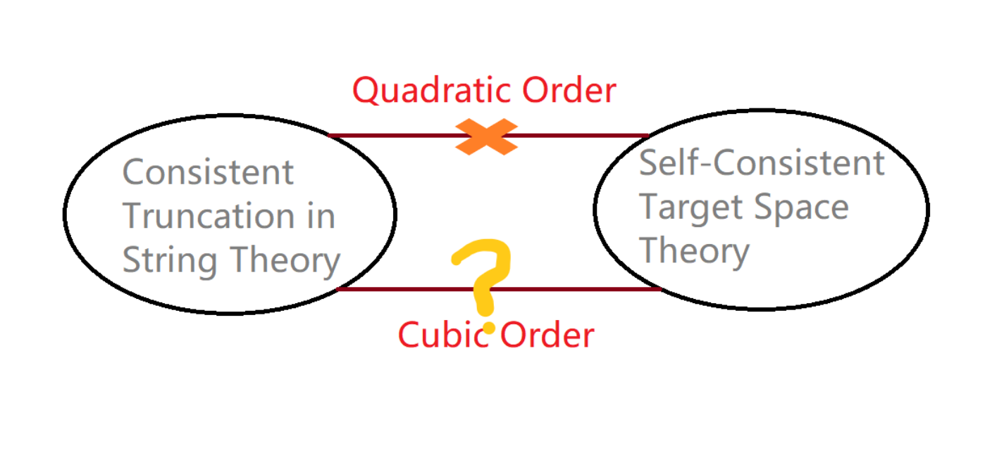
In this paper, we derive the cubic action from Double Field Theory for $N_{L}+N_{R}=2$ . For $(N_{L},N_{R})=(1,1)$ , the fluctuation fields are: $h_{jk}(x^{\mu},x^{a},\tilde{x}_{a})$ ; $b_{jk}(x^{\mu},x^{a},\tilde{x}_{a})$ ; $\phi(x^{\mu},x^{a},\tilde{x}_{a})$ , where $j,k=1,2,\cdots,D$ . Here $D$ is the number of compact and non-compact directions. In the bosonic string theory, it results $D=26$ . For the massive states $(N_{L},N_{R})=(2,0);(0,2)$ , the field strength associated with a one-form field replaces the $b_{jk}$ . A well-known problem in Double Field Theory is no consistent truncation of massive states. The quadratic-order corresponds to the non-interacting theory. It is unnecessary to have the interaction between the different modes [21]. Writing a self-consistent theory for each mode does not suffer any problems. The non-linear term should give the non-trivial constraints to the infinite summation for different numbers of $N_{L}$ and $N_{R}$ . We show this problem in Fig. 1.

Refer to caption — Figure 1: We show the problem between String Theory and its target space.

We use the gauge symmetry with the constraint for each $\lambda$ to show the cubic action. Therefore, the consistent truncation does not bother with the self-consistency of target space theory. To summarize our results:

•

We generalize the constraint for $\lambda\neq 0$ compatible with the integration by part. It shows the unique generalization. Products are commutative. For $\lambda=0$ , the constraint annihilates half of the degrees of freedom. Massive states do not follow the strong constraint.
•

The cubic action for $(N_{L},N_{R})=(1,1)$ corresponds to $\lambda=0$ . One can replace the massless two-form field with the field strength associated with the one-form field. Therefore, one can obtain the gauge transformation for the massive states by the one-to-one correspondence. Hence we can derive the cubic action for the spin-2 Fierz-Pauli fields or $(N_{L},N_{R})=(2,0);(0,2)$ . We obtain the gauge-invariant action by introducing the additional coupling between the one-form field and other fields.
•

We finally show that none of such new solutions allow both momentum and winding modes in the case of one double direction.

The organization of this paper is as follows: We generalize the constraint to $\lambda\neq 0$ in Sec. 2. We then show the closed gauge transformation in Sec. 3. The result of the quadratic and cubic orders for the action is in Sec. 4 and Sec. 5. We show that one double direction is not enough for Double Field Theory in Sec. 6. In the end, we discuss our results and conclude in Sec. 7. We show the closed gauge transformation of the generalized metric in Appendix A. The derivation of the cubic action is in Appendix B.

2 Constraint

We define the constraint [15] and show the generalization to the multiple products.

2.1 Definition

The constraint is [15]

\displaystyle\partial_{M}\partial^{M}f=-\lambda f,

(12)

where

\displaystyle\partial_{M}\equiv\begin{pmatrix}\,\tilde{\partial}^{m}\,\\[2.58334pt] {\partial_{m}}\end{pmatrix}.

(13)

We label the doubled indices by $M=1,2,\cdots,2D$ . We then raise or lower the doubled indices by the O( $D$ , $D$ ) metric [15, 16, 17]

\displaystyle\eta=\begin{pmatrix}0&I\\ I&0\end{pmatrix}.

(14)

We implement the constraint on the momentum space as follows. The star product provides the convenient notation

\displaystyle A*1\equiv\sum_{K}A_{K}\exp(iKX)\delta_{KK,\lambda},

(15)

where

\displaystyle X^{M}\equiv(\tilde{x}_{j},x^{j}),\qquad K^{M}\equiv(p_{j},\omega^{j});

(16)

\displaystyle KK\equiv K^{M}K_{M},\qquad KX\equiv K^{M}X_{M}.

(17)

This notation distinguishes $A$ from $A*1$ . Although the notation is unique, it is not manageable for being explicitly written all the time. Therefore, we will assume that all doubled fields satisfy the constraints in deriving quadratic and cubic actions. The $x^{j}$ ’s and $\tilde{x}_{j}$ ’s are the compact coordinate and the dual, respectively. The $p_{j}$ ’s and $\omega^{j}$ ’s are the momenta and windings along with the compact directions, respectively. This product imposes a constraint on $A$

\displaystyle\partial^{M}\partial_{M}(A*1)=-\lambda(A*1)

(18)

that is the only one required in deriving the quadratic action. A higher number of products is necessary when interested in higher orders. Therefore, we first discuss the quadratic products for the quadratic action.

2.2 Quadratic Action

The integration by part shows the constraint

\displaystyle K_{A}+K_{B}=0

(19)

for the quadratic term

\displaystyle\int[dxd\tilde{x}]\ A*B.

(20)

Therefore, we obtain

\displaystyle K_{A}K_{B}=-K_{A}^{2}=-\lambda.

(21)

Hence the quadratic products are:

\displaystyle A*B=B*A\equiv\sum_{K_{A},K_{B}}A_{K_{A}}B_{K_{B}}\exp\big(i(K_{A}+K_{B})X\big)\delta_{K_{A}K_{A},\lambda}\delta_{K_{B}K_{B},\lambda}\delta_{K_{A}K_{B},-\lambda}.

(22)

When $\lambda$ vanishes, the constraint reduces to the strong constraint. The quadratic products satisfy the constraint

\displaystyle\partial_{M}\partial^{M}(A*B)=0

(23)

for each $\lambda$ . The restriction implies that the quadratic action satisfies the constraint as the strong constraint case. Because the field still satisfies the relaxed constraint, the constraint of quadratic products does not prohibit the non-orthogonality of momenta. Integrating by part also provides the following equality

\displaystyle\int[dxd\tilde{x}]\ A*B=\int[dxd\tilde{x}]\ AB.

(24)

For massive states, $\lambda$ still leads to the possibility of going beyond String Theory.

2.3 Cubic Action

For the cubic action, the integration by part also shows the similar constraint

\displaystyle K_{A}+K_{B}+K_{C}=0

(25)

from the following integration:

\displaystyle\int[dxd\tilde{x}]\ (A*B)*C;\qquad\int[dxd\tilde{x}]\ A*(B*C).

(26)

Each momentum satisfies the condition:

\displaystyle K_{A}^{2}=K_{B}^{2}=K_{C}^{2}=\lambda.

(27)

Hence we obtain:

	$\displaystyle K_{A}K_{B}=K_{A}K_{C}=K_{B}K_{C}=-\frac{\lambda}{2},$
	$\displaystyle(K_{A}+K_{B})K_{C}=(K_{A}+K_{C})K_{B}=(K_{B}+K_{C})K_{A}=-\lambda;$		(28)

\displaystyle\partial_{M}A*\partial^{M}B=\frac{\lambda}{2}A*B,\qquad\partial_{M}A*\partial^{M}C=\frac{\lambda}{2}A*C,\qquad\partial_{M}B*\partial^{M}C=\frac{\lambda}{2}B*C,

(29)

	$\displaystyle\partial_{M}(AB)\partial^{M}C=\lambda(AB)C,$
	$\displaystyle\partial_{M}(AC)\partial^{M}B=\lambda(AC)B,$
	$\displaystyle\partial_{M}(BC)\partial^{M}A=\lambda(BC)A.$		(30)

The triple products are associative:

	$\displaystyle A(BC)$	(31)
$\displaystyle=$	$\displaystyle(AB)C$
$\displaystyle\equiv$	$\displaystyle\sum_{K_{A},K_{B},K_{C}}A_{K_{A}}B_{K_{B}}C_{K_{C}}\exp\big(i(K_{A}+K_{B}+K_{C})X\big)$
	$\displaystyle\times\delta_{K_{A}K_{A},\lambda}\delta_{K_{B}K_{B},\lambda}\delta_{K_{C}K_{C},\lambda}\delta_{K_{A}K_{B},-\frac{\lambda}{2}}\delta_{K_{A}K_{C},-\frac{\lambda}{2}}.$

The triple products also satisfy the constraint:

\displaystyle\partial^{M}\partial_{M}\big(A*(B*C)\big)=0

(32)

for each $\lambda$ . It implies that the cubic action has a similar situation to the quadratic action. One can unify the cubic and quadratic action by writing

\displaystyle\partial_{M}(A*1)\partial^{M}C=\lambda(A*1)*C.

(33)

For the convenient notation, we will not write the quadratic action in terms of the triple products.

2.4 Quadruple Products

For the quadruple products, the integration by part shows:

\displaystyle K_{A}+K_{B}+K_{C}+K_{D}=0,

(34)

and the level matching condition gives:

\displaystyle K_{A}^{2}=K_{B}^{2}=K_{C}^{2}=K_{D}^{2}=\lambda.

(35)

The momenta satisfy:

	$\displaystyle K_{A}K_{B}+K_{A}K_{C}+K_{B}K_{C}=K_{A}K_{B}+K_{A}K_{D}+K_{B}K_{D}$	(36)
$\displaystyle=$	$\displaystyle K_{A}K_{C}+K_{A}K_{D}+K_{C}K_{D}=K_{B}K_{C}+K_{B}K_{D}+K_{C}K_{D}$
$\displaystyle=$	$\displaystyle-\lambda.$

It is easy to observe that:

\displaystyle(K_{A}+K_{B})K_{C}=-\lambda-K_{A}K_{B};\qquad(K_{B}+K_{C})K_{A}=-\lambda-K_{B}K_{C}.

(37)

Therefore, the triple products are not associated here with the quadruple action. A general simplification is only up to our concern (cubic action).

3 Gauge Transformation

We apply the constraint to realize the non-linear gauge transformation. The product is only commutative up to triple products. It implies that some field configurations should have the gauge symmetry, defined by the commutative product. Hence the non-linear realization should provide non-trivial evidence to the constraint. The non-vanishing $\lambda$ goes beyond the strong constraint. Showing a closed gauge transformation is already non-trivial. It is also general enough for a cubic action.

Here we discuss the generalized metric [5] and the scalar dilaton:

\displaystyle{\cal H}_{MN}\equiv\begin{pmatrix}g^{-1}&-g^{-1}*{\mbox{b}}\\ {\mbox{b}}*g^{-1}&g-{\mbox{b}}*g^{-1}*{\mbox{b}}\end{pmatrix};\qquad\Phi=e^{-2\phi}*\sqrt{|\mbox{det}g|}.

(38)

Here $g_{jk}$ is a symmetric tensor field, and ${\mbox{b}}_{jk}$ is an anti-symmetric tensor field. The generalized metric combines the symmetric and anti-symmetric components into one symmetric structure.

The gauge transformations are:

	$\displaystyle\delta_{\xi}{\cal H}^{MN}$	$\displaystyle=$	$\displaystyle\xi^{P}\partial_{P}{\cal H}^{MN}+\big(\partial^{M}\xi_{P}-\partial_{P}\xi^{M}\big){\cal H}^{PN}+\big(\partial^{N}\xi_{P}-\partial_{P}\xi^{N})*{\cal H}^{MP};$
	$\displaystyle\delta_{\xi}\Phi$	$\displaystyle=$	$\displaystyle-\frac{1}{2}\partial_{M}\xi^{M}+\xi^{M}*\partial_{M}\Phi,$		(39)

where the gauge parameter $\xi_{P}$ is

\displaystyle\xi^{P}\equiv\begin{pmatrix}\tilde{\xi}_{j}\\ \xi^{j}\end{pmatrix}.

(40)

The vector field $\xi^{j}$ generates the diffeomorphism while another component provides a dual one. The scalar dilaton for the fluctuation level becomes

\displaystyle\exp(-2\Phi)\equiv\exp(-2\phi)\sqrt{-\det h_{jk}}.

(41)

We show the closed gauge transformation for the scalar dilaton. The computation is as in the following:

	$\displaystyle[\delta_{\xi_{1}},\delta_{\xi_{2}}]_{*}\Phi$	(42)
$\displaystyle\equiv$	$\displaystyle-\frac{1}{2}\xi_{2}^{M}\partial_{M}\partial_{P}\xi_{1}^{P}+\xi_{2}^{M}\partial_{M}\xi_{1}^{P}\partial_{P}\Phi+\frac{1}{2}\xi_{1}^{M}\partial_{M}\partial_{P}\xi_{2}^{P}-\xi_{1}^{M}\partial_{M}\xi_{2}^{P}\partial_{P}\Phi$
	$\displaystyle+\xi_{2}^{M}\xi_{1}^{P}\partial_{M}\partial_{P}\Phi-\xi_{1}^{M}\xi_{2}^{P}\partial_{M}\partial_{P}\Phi$
$\displaystyle=$	$\displaystyle-\frac{1}{2}\xi_{2}^{M}\partial_{M}\partial_{P}\xi_{1}^{P}+\xi_{2}^{M}\partial_{M}\xi_{1}^{P}\partial_{P}\Phi+\frac{1}{2}\xi_{1}^{M}\partial_{M}\partial_{P}\xi_{2}^{P}-\xi_{1}^{M}\partial_{M}\xi_{2}^{P}\partial_{P}\Phi$
$\displaystyle=$	$\displaystyle\frac{1}{2}\partial_{M}[\xi_{1},\xi_{2}]_{C}^{M}-[\xi_{1},\xi_{2}]^{M}_{C}\partial_{M}\Phi$
$\displaystyle=$	$\displaystyle-\delta_{[\xi_{1},\xi_{2}]_{C}}\Phi.$

Here the $C$ -bracket is:

\displaystyle[\xi_{1},\xi_{2}]_{C}^{M}\equiv\xi^{N}_{[1}*\partial_{N}\xi^{M}_{2]}-\frac{1}{2}\xi^{P}_{[1}*\partial^{M}\xi_{2]P},\ [j,k]\equiv jk-kj.

(43)

We used following results in the calculation:

	$\displaystyle\partial_{M}[\xi_{1},\xi_{2}]_{C}^{M}$	(44)
$\displaystyle=$	$\displaystyle\partial_{M}\bigg(\xi_{1}^{N}\partial_{N}\xi_{2}^{M}-\xi_{2}^{N}\partial_{N}\xi_{1}^{M}-\frac{1}{2}\eta^{MN}\eta_{PQ}\xi_{1}^{P}\partial_{N}\xi_{2}^{Q}+\frac{1}{2}\eta^{MN}\eta_{PQ}\xi_{2}^{P}\partial_{N}\xi_{1}^{Q}\bigg)$
$\displaystyle=$	$\displaystyle\partial_{M}\xi_{1}^{N}\partial_{N}\xi_{2}^{M}+\xi_{1}^{N}\partial_{M}\partial_{N}\xi_{2}^{M}-\partial_{M}\xi_{2}^{N}\partial_{N}\xi_{1}^{M}-\xi_{2}^{N}\partial_{M}\partial_{N}\xi_{1}^{M}$
	$\displaystyle-\frac{1}{2}\partial_{M}\xi_{1}^{P}\partial^{M}\xi_{2,P}-\frac{1}{2}\xi_{1}^{P}\partial_{M}\partial^{M}\xi_{2,P}+\frac{1}{2}\partial_{M}\xi_{2}^{P}\partial^{M}\xi_{1,P}+\frac{1}{2}\xi_{2}^{P}\partial_{M}\partial^{M}\xi_{1,P}$
$\displaystyle=$	$\displaystyle\xi_{1}^{N}\partial_{M}\partial_{N}\xi_{2}^{M}-\xi_{2}^{N}\partial_{M}\partial_{N}\xi_{1}^{M}-\frac{\lambda}{4}\xi_{1}^{P}\xi_{2,P}+\frac{\lambda}{2}\xi_{1}^{P}\xi_{2,P}+\frac{\lambda}{4}\xi_{2}^{P}\xi_{1,P}-\frac{\lambda}{2}\xi_{2}^{P}\xi_{1,P}$
$\displaystyle=$	$\displaystyle\xi_{1}^{N}\partial_{M}\partial_{N}\xi_{2}^{M}-\xi_{2}^{N}\partial_{M}\partial_{N}\xi_{1}^{M};$

	$\displaystyle-[\xi_{1},\xi_{2}]^{M}_{C}*\partial_{M}\Phi$	(45)
$\displaystyle=$	$\displaystyle-\bigg(\xi_{1}^{N}\partial_{N}\xi_{2}^{M}-\xi_{2}^{N}\partial_{N}\xi_{1}^{M}-\frac{1}{2}\eta^{MN}\eta_{PQ}\xi_{1}^{P}\partial_{N}\xi_{2}^{Q}+\frac{1}{2}\eta^{MN}\eta_{PQ}\xi_{2}^{P}\partial_{N}\xi_{1}^{Q}\bigg)*\partial_{M}\Phi$
$\displaystyle=$	$\displaystyle\xi_{2}^{M}\partial_{M}\xi_{1}^{P}\partial_{P}\Phi-\xi_{1}^{M}\partial_{M}\xi_{2}^{P}\partial_{P}\Phi$
	$\displaystyle+\frac{1}{2}\xi_{1}^{P}\partial^{M}\xi_{2,P}\partial_{M}\Phi-\frac{1}{2}\xi_{2}^{P}\partial^{M}\xi_{1,P}\partial_{M}\Phi$
$\displaystyle=$	$\displaystyle\xi_{2}^{M}\partial_{M}\xi_{1}^{P}\partial_{P}\Phi-\xi_{1}^{M}\partial_{M}\xi_{2}^{P}\partial_{P}\Phi.$

The quadratic products have a non-unique notation in our paper. Here we use:

\displaystyle\partial_{M}{\cal A}*\partial^{M}{\cal C}=\frac{\lambda}{2}{\cal A}*{\cal C}\neq\lambda{\cal A}*{\cal C}.

(46)

For the generalized metric, the gauge transformation is also closed similarly

\displaystyle[\delta_{\xi_{1}},\delta_{\xi_{2}}]_{*}{\cal H}^{MN}=-\delta_{[\xi_{1},\xi_{2}]_{*}}{\cal H}^{MN}.

(47)

We write the details in Appendix A. Our result implies that the gauge transformations of the cubic action are also closed under the constraint.

4 Quadratic Theory

We first discuss the field content for $N_{L}+N_{R}=2$ . We then derive the quadratic action from the gauge transformation. Both appearances of momentum and winding modes generate a mass term.

4.1 Field Content

The choices of $N_{L}$ and $N_{R}$ are $(N_{L},N_{R})=(1,1);(2,0);(0,2)$ . For the massless state $(N_{L},N_{R})=(1,1)$ , the first-excited state is $\alpha_{-1}^{j}\bar{\alpha}_{-1}^{k}|0\rangle$ , where $\alpha_{-1}^{j}$ is the left creation operator, and $\bar{\alpha}_{-1}^{k}$ is the right one. It generates a symmetric traceless tensor field $h_{jk}$ with $(D-2)(D-1)/2-1$ physical degrees of freedom; a scalar field $\phi$ with one physical degree of freedom; an anti-symmetric tensor field $b_{jk}$ with $(D-2)(D-3)/2$ physical degrees of freedom. The number of total physical degrees of freedom is $(D-2)^{2}$ . It forms the massless particle’s representation of SO( $D-2$ ). The spin-2 Fierz-Pauli fields with the Lorentz symmetry form the representation of SO( $D-1$ ). Later we will show that the massive states $(N_{L},N_{R})=(2,0);(0,2)$ correspond to the spin-2 Fierz-Pauli fields.

For $(N_{L},N_{R})=(2,0)$ , the first excited states are $\alpha_{-1}^{j}\alpha_{-1}^{k}|0\rangle$ and $\alpha_{-2}^{j}|0\rangle$ . The operator $\alpha_{-1}^{j}\alpha_{-1}^{k}$ generates a symmetric traceless tensor field $h_{jk}$ with $(D-2)(D-1)/2-1$ physical degrees of freedom; a scalar field $\phi$ with one physical degree of freedom. The operator $\alpha_{-2}^{j}$ generates a one-form gauge field $A_{j}$ with $D-2$ physical degrees of freedom. Hence the number of total physical degrees of freedom is $(D-2)(D+1)/2$ . This number is the same as the dimension of the traceless symmetric tensor of SO( $D-1$ ). We conclude that the massive state is spin-2. For $(N_{L}=0,N_{R}=2)$ , we replace the left creation field with the right one. The result remains the same. We determine the allowed momentum and winding numbers by the level matching condition

\displaystyle N_{L}-N_{R}=n_{a}m_{a}.

(48)

For massive states with one compactified direction, the allowed momentum and winding numbers are:

	$\displaystyle(N_{L},N_{R})=(2,0),\ (n,m)=(1,2),(2,1),(-1,-2),(-2,-1);$
	$\displaystyle(N_{L},N_{R})=(0,2),\ (n,m)=(-1,-2),(-2,-1),(1,-2),(2,-1).$		(49)

4.2 Quadratic Action

We consider the fluctuations around the constant symmetric and the vanishing anti-symmetric backgrounds. The quadratic action for the massless state $(N_{L}=1,N_{R}=1)$ is [15]

	$\displaystyle S^{(2)}_{DFT}$	(50)
$\displaystyle=$	$\displaystyle\frac{1}{16\pi G_{N}}\int[dxd\tilde{x}]\ \bigg(\frac{1}{4}h^{jk}\partial_{l}\partial^{l}h_{jk}+\frac{1}{2}\partial^{j}h_{jk}\partial_{l}h^{lk}-2\Phi\partial^{j}\partial^{k}h_{jk}-4\Phi\partial^{j}\partial_{j}\Phi$
	$\displaystyle+\frac{1}{4}h^{jk}\tilde{\partial}_{l}\tilde{\partial}^{k}h_{jk}+\frac{1}{2}\tilde{\partial}^{j}h_{jl}\tilde{\partial}_{k}h^{kl}+2\Phi\tilde{\partial}^{j}\tilde{\partial}^{k}h_{jk}-4\Phi\tilde{\partial}^{j}\tilde{\partial}_{j}\Phi$
	$\displaystyle+\frac{1}{4}b^{jk}\partial^{l}\partial_{l}b_{jk}+\frac{1}{2}\partial^{k}b_{jk}\partial_{l}b^{jl}+\frac{1}{4}b^{jk}\tilde{\partial}^{l}\tilde{\partial}_{l}b_{jk}+\frac{1}{2}\tilde{\partial}^{k}b_{jk}\tilde{\partial}_{l}b^{jl}$
	$\displaystyle+(\partial_{k}h^{jk})\tilde{\partial}^{l}b_{jl}+(\tilde{\partial}^{l}h_{jl})\partial_{k}b^{jk}-4\Phi\partial^{j}\tilde{\partial}^{k}b_{jk}\bigg),$

where $G_{N}$ is the gravitational constant. The integration $\int[dxd\tilde{x}]$ is over all of the $n+2d$ coordinates of $\mathbb{R}^{n-1,1}\times T^{2d}$ . The periodic coordinates of the doubled torus are $(x^{a},\tilde{x}_{a})$ . We will write an analogous action for the massive states from $S^{(2)}_{DFT}$ . Here all fluctuation fields also satisfy the constraint. Therefore, we should use the star product in the quadratic action. We should also use the triple way to rewrite the quadratic product for a unique notation. However, keeping in mind that the double fields always satisfy the constraint of the cubic action. We will use the simplified notation (but non-unique) to simplify the derivation.

The gauge transformation of $S^{(2)}_{DFT}$ is a linear doubled diffeomorphism [15]:

$\displaystyle\delta h_{jk}$	$\displaystyle=$	$\displaystyle\partial_{j}\epsilon_{k}+\partial_{k}\epsilon_{j}+\tilde{\partial}_{j}\tilde{\epsilon}_{k}+\tilde{\partial}_{k}\tilde{\epsilon}_{j};$
$\displaystyle\delta b_{jk}$	$\displaystyle=$	$\displaystyle-\big(\tilde{\partial}_{j}\epsilon_{k}-\tilde{\partial}_{k}\epsilon_{j}\big)-\big(\partial_{j}\tilde{\epsilon}_{k}-\partial_{k}\tilde{\epsilon}_{j}\big);$
$\displaystyle\delta\Phi$	$\displaystyle=$	$\displaystyle-\frac{1}{2}(\partial_{j}\epsilon^{j}-\tilde{\partial}_{j}\tilde{\epsilon}^{j}).$	(51)

When the gauge parameters and fields are independent of $\tilde{x}_{j}$ , the doubled diffeomorphism reduces to the standard one.

The fields associated with $(N_{L}=2,N_{R}=0)$ and $(N_{L}=0,N_{R}=2)$ are: a symmetric traceless tensor $h_{jk}(x^{\mu},x^{a},\tilde{x}_{a})$ ; a one-form gauge field $A_{j}(x^{\mu},x^{a},\tilde{x}_{a})$ ; a scalar dilaton field $\Phi(x^{\mu},x^{a},\tilde{x}_{a})$ . We define the field strength associated with the one-form gauge field $A_{j}$ is:

\displaystyle b_{jk}=-\big(\tilde{\partial}_{j}A_{k}-\tilde{\partial}_{k}A_{j}\big)+\big(\partial_{k}A_{j}-\partial_{j}A_{k}\big).

(52)

The gauge transformation of $A_{j}$ is:

\displaystyle\delta A_{j}=\epsilon_{j}=\tilde{\epsilon}_{j}.

(53)

Therefore, the field strength has the same gauge transformation as the anti-symmetric field for $(N_{L},N_{R})=(1,1)$ . This result implies $\epsilon_{j}=\tilde{\epsilon}_{j}$ . Later we will show that the gauge invariance leads to the assumption. Hence a one-to-one correspondence of the fields for the massive and massless states [15]. It allows us to consider the quadratic action (50) as our starting point for the massive states. When one applies the correspondence to the massless theory, we also change the notation

\displaystyle S^{(2)}_{DFT}\rightarrow\tilde{S}^{(2)}_{new}

(54)

Here we distinguish the massless and massive quadratic actions because their field contents are different.

Since $\tilde{S}^{(2)}_{new}$ is gauge invariant for $\lambda=0$ , it is only necessary to show the calculation for $\lambda\neq 0$ . The gauge transformation for the $\tilde{S}^{(2)}_{new}$ is:

	$\displaystyle\delta\tilde{S}^{(2)}_{new}$	(55)
$\displaystyle=$	$\displaystyle\frac{1}{16\pi G_{N}}\int[dxd\tilde{x}]\ \bigg(\partial^{j}\tilde{\partial}_{j}\tilde{\epsilon}_{l}\partial_{k}h^{kl}-4\Phi\partial^{j}\partial^{k}\tilde{\partial}_{j}\tilde{\epsilon}_{k}+\partial^{j}\tilde{\partial}_{j}\epsilon_{l}\tilde{\partial}_{k}h^{kl}+4\Phi\tilde{\partial}^{j}\tilde{\partial}^{k}\partial_{j}\epsilon_{k}$
	$\displaystyle+\partial^{k}\tilde{\partial}_{k}\epsilon_{j}\partial_{l}b^{jl}+\partial^{k}\tilde{\partial}_{k}\tilde{\epsilon}_{j}\tilde{\partial}_{l}b^{jl}+(\partial_{l}\tilde{\partial}^{l}\tilde{\epsilon}^{j})\tilde{\partial}^{k}b_{jk}+(\partial_{l}\tilde{\partial}^{l}\epsilon^{j})\partial^{k}b_{jk}$
	$\displaystyle+(\partial_{l}h^{jl})\tilde{\partial}^{k}\partial_{k}\tilde{\epsilon}_{j}+(\tilde{\partial}_{l}h^{jl})\tilde{\partial}^{k}\partial_{k}\epsilon_{j}+4\Phi\partial^{j}\tilde{\partial}^{k}\tilde{\partial}_{j}\epsilon_{k}-4\Phi\partial^{j}\tilde{\partial}^{k}\partial_{k}\tilde{\epsilon}_{j}\bigg)$
$\displaystyle=$	$\displaystyle\frac{1}{16\pi G_{N}}\int[dxd\tilde{x}]\ \bigg(-\frac{\lambda}{2}\tilde{\epsilon}_{l}\partial_{k}h^{kl}+2\lambda\Phi\partial^{k}\tilde{\epsilon}_{k}-\frac{\lambda}{2}\epsilon_{l}\tilde{\partial}_{k}h^{kl}-2\lambda\Phi\tilde{\partial}^{k}\epsilon_{k}$
	$\displaystyle-\frac{\lambda}{2}\epsilon_{j}\partial_{l}b^{jl}-\frac{\lambda}{2}\tilde{\epsilon}_{j}\tilde{\partial}_{l}b^{jl}-\frac{\lambda}{2}\tilde{\epsilon}^{j}\tilde{\partial}^{k}b_{jk}-\frac{\lambda}{2}\epsilon^{j}\partial^{k}b_{jk}$
	$\displaystyle-\frac{\lambda}{2}\tilde{\epsilon}_{j}\partial_{l}h^{jl}-\frac{\lambda}{2}\epsilon_{j}\tilde{\partial}_{l}h^{jl}-2\lambda\Phi\tilde{\partial}^{k}\epsilon_{k}+2\lambda\Phi\partial^{j}\tilde{\epsilon}_{j}\bigg)$
$\displaystyle=$	$\displaystyle\frac{1}{16\pi G_{N}}\int[dxd\tilde{x}]\ \bigg(-\lambda\tilde{\epsilon}_{l}\partial_{k}h^{kl}-\lambda\epsilon_{l}\tilde{\partial}_{k}h^{kl}-\lambda\epsilon_{j}\partial_{l}b^{jl}-\lambda\tilde{\epsilon}_{j}\tilde{\partial}_{l}b^{jl}$
	$\displaystyle+4\lambda\Phi\partial^{k}\tilde{\epsilon}_{k}-4\lambda\Phi\tilde{\partial}^{k}\epsilon_{k}\bigg)$
$\displaystyle=$	$\displaystyle\frac{1}{16\pi G_{N}}\int[dxd\tilde{x}]\ \bigg(-\lambda\tilde{\epsilon}_{j}\partial_{k}(h^{jk}+b^{jk})-\lambda\epsilon_{j}\tilde{\partial}_{k}(h^{jk}+b^{jk})+4\lambda\Phi(\partial^{k}\tilde{\epsilon}_{k}-\tilde{\partial}^{k}\epsilon_{k})\bigg)$
$\displaystyle=$	$\displaystyle\frac{1}{16\pi G_{N}}\int[dxd\tilde{x}]\ \bigg(\lambda(h^{jk}+b^{jk})(\partial_{k}\tilde{\epsilon}_{j}+\tilde{\partial}_{k}\epsilon_{j})+4\lambda\Phi(\partial^{k}\tilde{\epsilon}_{k}-\tilde{\partial}^{k}\epsilon_{k})\bigg)$
$\displaystyle=$	$\displaystyle\frac{1}{16\pi G_{N}}\int[dxd\tilde{x}]\ \bigg(\frac{\lambda}{2}b^{jk}(\partial_{k}\tilde{\epsilon}_{j}-\partial_{j}\tilde{\epsilon}_{k}+\tilde{\partial}_{k}\epsilon_{j}-\tilde{\partial}_{j}\epsilon_{k})+\lambda h^{jk}(\partial_{k}\tilde{\epsilon}_{j}+\tilde{\partial}_{k}\epsilon_{j})$
	$\displaystyle+4\lambda\Phi(\partial^{k}\tilde{\epsilon}_{k}-\tilde{\partial}^{k}\epsilon_{k})\bigg)$
$\displaystyle=$	$\displaystyle\frac{1}{16\pi G_{N}}\int[dxd\tilde{x}]\ \bigg(\frac{\lambda}{4}\delta(b^{jk}b_{jk})+\lambda h^{jk}(\partial_{k}\tilde{\epsilon}_{j}+\tilde{\partial}_{k}\epsilon_{j})+4\lambda\Phi(\partial^{k}\tilde{\epsilon}_{k}-\tilde{\partial}^{k}\epsilon_{k})\bigg).$

The result of gauge transformation shows the non-invariant terms. The constraint

\displaystyle\partial^{j}\tilde{\partial}_{j}f=-\frac{\lambda}{2}f

(56)

cannot annihilate these terms. Hence it is necessary to introduce the new term to restore the gauge symmetry. Now we assume that

\displaystyle\epsilon_{j}=\tilde{\epsilon}_{j}.

(57)

We then obtain:

	$\displaystyle\delta\tilde{S}^{(2)}_{new}$	(58)
$\displaystyle=$	$\displaystyle\frac{1}{16\pi G_{N}}\int[dxd\tilde{x}]\ \bigg(\frac{\lambda}{4}\delta(b^{jk}b_{jk})+\lambda h^{jk}(\partial_{k}\tilde{\epsilon}_{j}+\tilde{\partial}_{k}\epsilon_{j})+4\lambda\Phi(\partial^{j}\tilde{\epsilon}_{j}-\tilde{\partial}^{j}\epsilon_{j})\bigg)$
$\displaystyle=$	$\displaystyle\frac{1}{16\pi G_{N}}\int[dxd\tilde{x}]\ \bigg(\frac{\lambda}{4}\delta(b^{jk}b_{jk})+\frac{\lambda}{2}h^{jk}\delta h_{jk}-8\lambda\Phi\delta\Phi\bigg)$
$\displaystyle=$	$\displaystyle\frac{1}{16\pi G_{N}}\int[dxd\tilde{x}]\ \bigg(\frac{\lambda}{4}\delta(b^{jk}b_{jk})+\frac{\lambda}{4}\delta(h^{jk}h_{jk})-4\lambda\delta(\Phi^{2})\bigg).$

The new term is

\displaystyle\tilde{S}^{(2)}_{add}=\frac{1}{16\pi G_{N}}\int[dxd\tilde{x}]\ \bigg(-\frac{\lambda}{4}b^{jk}b_{\mu\nu}-\frac{\lambda}{4}h^{jk}h_{jk}+4\lambda\Phi^{2}\bigg).

(59)

The quadratic action for the massive states is:

	$\displaystyle\tilde{S}^{(2)}_{DFT}$	$\displaystyle=$	$\displaystyle\tilde{S}^{(2)}_{new}+\tilde{S}^{(2)}_{add}$		(60)
		$\displaystyle=$	$\displaystyle\tilde{S}^{(2)}_{new}+\frac{1}{16\pi G_{N}}\int[dxd\tilde{x}]\ \bigg(-\frac{\lambda}{4}b^{jk}b_{jk}-\frac{\lambda}{4}h^{jk}h_{jk}+4\lambda\Phi^{2}\bigg).$		(60)

The gauge invariance requires the equality of the gauge parameters. It is consistent with the gauge transformation of the one-form gauge field. The constraint of the gauge parameters implies that the target space and its dual are not independent.

When the dilaton field vanishes, the scalar dilaton field at the quadratic order is

\displaystyle\Phi=-\frac{h^{j}{}_{j}}{4}.

(61)

The familiar graviton mass term $\lambda\big(h^{jk}h_{jk}-(h^{j}{}_{j})^{2}\big)$ appears in the quadratic theory. The non-vanishing $\lambda$ is due to $N_{L}\neq N_{R}$ . It implies that the mass term is due to the simultaneous appearance of the momentum and winding modes. From the point of view of non-compact lower-dimensional spacetime, the squared mass of the graviton is

\displaystyle{\cal M}_{g}^{2}=p^{2}+\omega^{2}+\frac{2(N_{L}-N_{R})}{\alpha^{\prime}}.

(62)

5 Cubic Theory

We first show the gauge transformation and then derive the cubic action. The gauge invariance requires the coupling between the one-form gauge field and other fields. Although Double Field Theory does not have a consistent truncation, the cubic target space theory is self-consistent for each mode. Hence we truncate other modes and get the self-consistent theory even if the issue of truncation exists. We provide the details for constructing the cubic action in Appendix B.

5.1 Gauge Transformation

The gauge transformation with $\epsilon_{j}=\tilde{\epsilon}_{j}$ are [15]:

\displaystyle\delta e_{jk}=2\bar{D}_{k}\epsilon_{j}+\big((D_{j}\epsilon^{l})e_{lk}-(D^{l}\epsilon_{j})e_{lk}+\epsilon_{l}D^{l}e_{jk}\big);\qquad\delta\Phi=-\frac{1}{2}D_{j}\epsilon^{j}+\epsilon_{j}D^{j}\Phi,

(63)

where

\displaystyle D_{k}\equiv\partial_{k}-\tilde{\partial}_{k};\qquad\bar{D}_{k}\equiv\partial_{k}+\tilde{\partial}_{k}.

(64)

The $e_{jk}$ is a non-linear combination of $h_{jk}$ and $b_{jk}$ [15]

\displaystyle e_{jk}=h_{jk}+b_{jk}+\cdots.

(65)

5.2 Cubic Action

We also begin from the massless cubic action

	$\displaystyle S_{DFT}^{(2)}+S_{DFT}^{(3)}$	(66)
$\displaystyle=$	$\displaystyle\int[dxd\tilde{x}]\ \bigg[\frac{1}{4}e_{jk}\Box e^{jk}+\frac{1}{4}(\bar{D}^{k}e_{jk})^{2}+\frac{1}{4}(D^{j}e_{jk})^{2}-2\Phi D^{j}\bar{D}^{k}e_{jk}-4\Phi\Box\Phi$
	$\displaystyle+\frac{1}{4}e_{jk}\bigg((D^{j}e_{lm})(\bar{D}^{k}e^{lm})-(D^{j}e_{lm})(\bar{D}^{m}e^{lk})-(D^{l}e^{jm})(\bar{D}^{k}e_{lm})\bigg)$
	$\displaystyle+\frac{1}{2}\Phi\bigg((D^{j}e_{jk})^{2}+(\bar{D}^{k}e_{jk})^{2}+\frac{1}{2}(D_{l}e_{jk})^{2}+\frac{1}{2}(\bar{D}_{l}e_{jk})^{2}+2e^{jk}(D_{j}D^{l}e_{lk}+\bar{D}_{k}\bar{D}^{l}e_{jl})\bigg)$
	$\displaystyle+4e_{jk}\Phi D^{j}\bar{D}^{k}\Phi+4\Phi^{2}\Box\Phi\bigg],$

where

\displaystyle\Box\equiv\frac{1}{2}(D^{2}+\bar{D}^{2}).

(67)

We use the same corresponding of the massless and massive fields. Up to the cubic order, the non-invariant terms are:

			$\displaystyle\delta\tilde{S}_{DFT}^{(2)}+\delta\tilde{S}_{new}^{(3)}$
		$\displaystyle=$	$\displaystyle\frac{\lambda}{16\pi G_{N}}\int[dxd\tilde{x}]\ \bigg[-\frac{1}{4}\delta(\Phi e^{lk}e_{lk})+4\delta(\Phi\Phi\Phi)+\frac{1}{2}\epsilon^{m}e_{mk}D_{l}e^{lk}+2\epsilon_{l}e^{lk}\bar{D}_{k}\Phi\bigg].$

For obtaining the gauge invariance, we need to add a new term

	$\displaystyle\tilde{S}_{add}^{(3)}$	(69)
$\displaystyle=$	$\displaystyle\frac{\lambda}{16\pi G_{N}}\int[dxd\tilde{x}]\ \bigg[\frac{1}{4}\Phi e^{lk}e_{lk}-4\Phi\Phi\Phi$
	$\displaystyle-\frac{1}{2}A^{m}e_{mk}D_{l}e^{lk}-2A_{l}e^{lk}\bar{D}_{k}\Phi+A^{m}\bar{D}_{k}(A_{m})D_{l}(e^{lk})+2\lambda A_{l}A^{l}\Phi\bigg].$

Hence we obtain the gauge symmetry for the massive state:

\displaystyle\delta\big(\tilde{S}_{DFT}^{(2)}+\tilde{S}_{new}^{(3)}+\tilde{S}_{add}^{(3)}\big)\equiv\delta\tilde{S}_{DFT}^{(2)}+\delta\tilde{S}_{DFT}^{(3)}=0.

(70)

The cubic action becomes:

	$\displaystyle\tilde{S}_{DFT}^{(2)}+\tilde{S}_{DFT}^{(3)}$	(71)
$\displaystyle=$	$\displaystyle\tilde{S}_{DFT}^{(2)}+\tilde{S}_{new}^{(3)}+\tilde{S}_{add}^{(3)}$
$\displaystyle=$	$\displaystyle\tilde{S}_{DFT}^{(2)}+\tilde{S}_{new}^{(3)}$
	$\displaystyle+\frac{\lambda}{16\pi G_{N}}\int[dxd\tilde{x}]\ \bigg[\frac{1}{4}\Phi e^{lk}e_{lk}-4\Phi\Phi\Phi$
	$\displaystyle-\frac{1}{2}A^{m}e_{mk}D_{l}e^{lk}-2A_{l}e^{lk}\bar{D}_{k}\Phi+A^{m}\bar{D}_{k}(A_{m})D_{l}(e^{lk})+2\lambda A_{l}A^{l}\Phi\bigg].$

We write the details in Appendix B.

6 $d=1$

The simplest solution should be for $d=1$ . For one double direction, the constraints are:

\displaystyle K_{A}^{2}=K_{B}^{2}=\lambda

(72)

give the momenta:

\displaystyle K_{A}=\begin{pmatrix}a\\ \frac{\lambda}{2a}\end{pmatrix};\qquad K_{B}=\begin{pmatrix}b\\ \frac{\lambda}{2b}\end{pmatrix},

(73)

where $a$ and $b$ are real-valued. The constraint for the product of the $K_{A}$ and $K_{B}$ is

\displaystyle K_{A}K_{B}=-\frac{\lambda}{2}

(74)

leads to the imaginary $a$ or $b$

\displaystyle\frac{a}{b}=\frac{-1\pm\sqrt{3}i}{2}.

(75)

Hence the contradiction shows no non-trivial solution for $d=1$ . In other words, the only solution satisfying the strong constraint exists. For $\lambda=0$ , ones can show the impossibility of the non-trivial solution [19, 20]. We generalize the proof to $\lambda\neq 0$ . Our proof only requires the quadratic products of momenta. Therefore, it doe not suffer from any ambiguity. Hence only for $d>1$ , it is possible to allow the massive states $\lambda\neq 0$ . The result also shows the difference between String Theory and Double Field Theory. Double Field Theory for $d=1$ only has the modes of $N_{L}=N_{R}$ . String Theory allows more states than Double Field Theory. The dual target spaces are relevant to the winding modes in Double Field Theory. Hence it gives more constraints to the choices of $N_{L}$ and $N_{R}$ .

7 Discussion and Conclusion

We derived the cubic action for $N_{L}+N_{R}=2$ in Double Field Theory [15]. With $N_{L}\neq N_{R}$ , the fields become massive. The field contents of the massive and massless cases have a one-to-one correspondence. Therefore, we could use the massless theory $(N_{L}=1,N_{R}=1)$ to build the massive case. From the perspective of String Theory, the constraints of fields should follow from the level matching condition. Therefore, the parameter [15]

\displaystyle\lambda=\frac{2(N_{L}-N_{R})}{\alpha^{\prime}}

(76)

generates the mass term and new interaction. We implemented the constraint to the triple products. Without being in contradiction with the integration by part, the generalization is unique. When one chooses $N_{L}\neq N_{R}$ , the momentum and winding modes do not vanish simultaneously. The interaction of the momentum and winding modes generates a massive graviton. Although $N_{L}<N_{R}$ gives the vacuum instability, the cubic interaction has an opposite sign to avoid the issue. The stable vacuum is possible, similar to spontaneous symmetry breaking. The massive theory relies on a solution with $\lambda\neq 0$ . We showed no such a solution for $d=1$ .

We obtained the massive gravity theory from $N_{L}\neq N_{R}$ . The non-linear deformation of massive gravity theory suffered from the issue of a ghost mode. Our theory respects String Theory. Therefore, the target space theory should be self-consistent. Hence one can apply our study to cosmology observation. The graviton mass is relevant to the interaction of the winding and momentum modes. It is possible to show the experimental constraint to $\alpha^{\prime}$ .

Up to the fluctuation level, it is hard to understand the perspective of geometry. We could realize the gauge symmetry up to the cubic order. Therefore, it is possible to extend our study to the generalized metric formulation [9]. For the massless theory, the generalized metric plays the role of manifest T-duality. The massive state should not have the O( $D$ , $D$ ) symmetric structure. However, one can always choose symmetric and anti-symmetric parts to form the generalized metric. It provides the convenient O( $D$ , $D$ ) indices to write action without changing the gauge transformation. One can explore the geometry by performing a similar analysis to the generalized metric formulation.

In the end, we comment on the consistent truncation. We first choose our consideration $N_{L}+N_{R}=2$ . The squared of mass is

\displaystyle{\cal M}^{2}=\frac{n^{2}}{R^{2}}+m^{2}\frac{R^{2}}{\alpha^{\prime 2}}.

(77)

We then compare the squared of mass to the $N_{L}+N_{R}=3$ case. One additional $1/\alpha^{\prime}$ term appears in the mass scale

\displaystyle{\cal M}^{2}=\frac{n^{2}}{R^{2}}+m^{2}\frac{R^{2}}{\alpha^{\prime 2}}+\frac{2}{\alpha^{\prime}}.

(78)

The choice $(n,m)=(2,1)$ in $N_{L}+N_{R}=2$ has a higher mass scale than $(n,m)=(1,3)$ in $N_{L}+N_{R}=3$ when the compactified radius is small enough

\displaystyle R^{2}\leq\frac{\alpha^{\prime}}{2}.

(79)

Hence concerning the $N_{L}+N_{R}=2$ is not enough for the consistent truncation (energy). The summation of infinite modes is necessary. This issue suggests that each mode in Double Field Theory cannot form a self-consistent theory. Since the quadratic-order corresponds to the non-interacting theory, one should expect gauge invariance for each mode. For the non-linear theory, it is hard to expect gauge invariance. Hence we extend our study to the cubic level. We can introduce the new coupling to show a gauge-invariant theory. Our results showed a contradiction to the expectation. Each mode can form a self-consistent target space theory even with no consistent truncation in String Theory.

Acknowledgments

The author thanks David S. Berman, Chi-Ming Chang, Xing Huang, Jeong-Hyuck Park, and Franco Pezzella for their discussion. The author also would like to thank for Nan-Peng Ma for his encouragement.

Chen-Te Ma acknowledges the China Postdoctoral Science Foundation, Postdoctoral General Funding: Second Class (Grant No. 2019M652926); Foreign Young Talents Program (Grant No. QN20200230017); Post-Doctoral International Exchange Program.

Appendix A Closed Gauge Transformation of
Generalized Metric

We provide the details to the gauge transformation of the generalized metric:

	$\displaystyle(\delta_{\xi_{1}}*\delta_{\xi_{2}}){\cal H}^{MN}$	(80)
$\displaystyle=$	$\displaystyle\xi_{2}^{P}\partial_{P}\xi_{1}^{Q}\partial_{Q}{\cal H}^{MN}+\xi_{2}^{P}\xi_{1}^{Q}\partial_{P}\partial_{Q}{\cal H}^{MN}$
	$\displaystyle+\xi_{2}^{P}\bigg(\partial_{P}\partial^{M}\xi_{1Q}-\partial_{P}\partial_{Q}\xi_{1}^{M}\bigg){\cal H}^{QN}+\xi_{2}^{P}\bigg(\partial^{M}\xi_{1Q}-\partial_{Q}\xi_{1}^{M}\bigg)\partial_{P}{\cal H}^{QN}$
	$\displaystyle+\xi_{2}^{P}\bigg(\partial_{P}\partial^{N}\xi_{1Q}-\partial_{P}\partial_{Q}\xi_{1}^{N}\bigg){\cal H}^{MQ}+\xi_{2}^{P}\bigg(\partial^{N}\xi_{1Q}-\partial_{Q}\xi_{1}^{N}\bigg)\partial_{P}{\cal H}^{MQ}$
	$\displaystyle+\bigg(\partial^{M}\xi_{2P}-\partial_{P}\xi_{2}^{M}\bigg)\xi_{1}^{Q}\partial_{Q}{\cal H}^{PN}$
	$\displaystyle+\bigg(\partial^{M}\xi_{2P}-\partial_{P}\xi_{2}^{M}\bigg)\bigg(\partial^{P}\xi_{1Q}-\partial_{Q}\xi_{1}^{P}\bigg){\cal H}^{QN}$
	$\displaystyle+\bigg(\partial^{M}\xi_{2P}-\partial_{P}\xi_{2}^{M}\bigg)\bigg(\partial^{N}\xi_{1Q}-\partial_{Q}\xi_{1}^{N}\bigg){\cal H}^{PQ}$
	$\displaystyle+\bigg(\partial^{N}\xi_{2P}-\partial_{P}\xi_{2}^{N}\bigg)\xi_{1}^{Q}\partial_{Q}{\cal H}^{PM}$
	$\displaystyle+\bigg(\partial^{N}\xi_{2P}-\partial_{P}\xi_{2}^{N}\bigg)\bigg(\partial^{P}\xi_{1Q}-\partial_{Q}\xi_{1}^{P}\bigg){\cal H}^{QM}$
	$\displaystyle+\bigg(\partial^{N}\xi_{2P}-\partial_{P}\xi_{2}^{N}\bigg)\bigg(\partial^{M}\xi_{1Q}-\partial_{Q}\xi_{1}^{M}\bigg){\cal H}^{PQ},$

	$\displaystyle[\delta_{\xi_{1}},\delta_{\xi_{2}}]_{*}{\cal H}^{MN}$	(81)
$\displaystyle=$	$\displaystyle\xi_{2}^{P}\partial_{P}\xi_{1}^{Q}\partial_{Q}{\cal H}^{MN}$
	$\displaystyle+\xi_{2}^{P}\bigg(\partial_{P}\partial^{M}\xi_{1Q}-\partial_{P}\partial_{Q}\xi_{1}^{M}\bigg){\cal H}^{QN}$
	$\displaystyle+\xi_{2}^{P}\bigg(\partial_{P}\partial^{N}\xi_{1Q}-\partial_{P}\partial_{Q}\xi_{1}^{N}\bigg){\cal H}^{MQ}$
	$\displaystyle+\bigg(\partial^{M}\xi_{2P}-\partial_{P}\xi_{2}^{M}\bigg)\bigg(\partial^{P}\xi_{1Q}-\partial_{Q}\xi_{1}^{P}\bigg){\cal H}^{QN}$
	$\displaystyle+\bigg(\partial^{N}\xi_{2P}-\partial_{P}\xi_{2}^{N}\bigg)\bigg(\partial^{P}\xi_{1Q}-\partial_{Q}\xi_{1}^{P}\bigg){\cal H}^{QM}$
	$\displaystyle-\xi_{1}^{P}\partial_{P}\xi_{2}^{Q}\partial_{Q}{\cal H}^{MN}$
	$\displaystyle-\xi_{1}^{P}\bigg(\partial_{P}\partial^{M}\xi_{2Q}-\partial_{P}\partial_{Q}\xi_{2}^{M}\bigg){\cal H}^{QN}-\xi_{1}^{P}\bigg(\partial_{P}\partial^{N}\xi_{2Q}-\partial_{P}\partial_{Q}\xi_{2}^{N}\bigg){\cal H}^{MQ}$
	$\displaystyle-\bigg(\partial^{M}\xi_{1P}-\partial_{P}\xi_{1}^{M}\bigg)\bigg(\partial^{P}\xi_{2Q}-\partial_{Q}\xi_{2}^{P}\bigg){\cal H}^{QN}$
	$\displaystyle-\bigg(\partial^{N}\xi_{1P}-\partial_{P}\xi_{1}^{N}\bigg)\bigg(\partial^{P}\xi_{2Q}-\partial_{Q}\xi_{2}^{P}\bigg){\cal H}^{QM}$
$\displaystyle=$	$\displaystyle-[\xi_{1},\xi_{2}]_{C}^{P}\partial_{P}{\cal H}^{MN}-\bigg(\partial^{M}[\xi_{1},\xi_{2}]_{CP}-\partial_{P}[\xi_{1},\xi_{2}]_{C}^{M}\bigg){\cal H}^{PN}$
	$\displaystyle-\bigg(\partial^{N}[\xi_{1},\xi_{2}]_{CP}-\partial_{P}[\xi_{1},\xi_{2}]_{C}^{N}\bigg)*{\cal H}^{MP}$
$\displaystyle=$	$\displaystyle-\delta_{[\xi_{1},\xi_{2}]_{C}}{\cal H}^{MN}.$

Therefore, the gauge transformation is closed. In the calculation, we used the following results:

	$\displaystyle-[\xi_{1},\xi_{2}]_{C}^{P}\partial_{P}{\cal H}^{MN}$	(82)
$\displaystyle=$	$\displaystyle-\bigg(\xi_{1}^{Q}\partial_{Q}\xi_{2}^{P}-\xi_{2}^{Q}\partial_{Q}\xi_{1}^{P}-\frac{1}{2}\eta^{PR}\eta_{OQ}\xi_{1}^{O}\partial_{R}\xi_{2}^{Q}+\frac{1}{2}\eta^{PR}\eta_{OQ}\xi_{2}^{O}\partial_{R}\xi_{1}^{Q}\bigg)*\partial_{P}{\cal H}^{MN}$
$\displaystyle=$	$\displaystyle\bigg(\xi_{2}^{Q}\partial_{Q}\xi_{1}^{P}-\xi_{1}^{Q}\partial_{Q}\xi_{2}^{P}\bigg)*\partial_{P}{\cal H}^{MN},$

			$\displaystyle-\bigg(\partial^{M}[\xi_{1},\xi_{2}]_{CP}-\partial_{P}[\xi_{1},\xi_{2}]_{C}^{M}\bigg)*{\cal H}^{PN}$
		$\displaystyle=$	$\displaystyle-\partial^{M}\bigg(\xi_{1}^{Q}\partial_{Q}\xi_{2P}-\xi_{2}^{Q}\partial_{Q}\xi_{1P}-\frac{1}{2}\eta_{OQ}\xi_{1}^{O}\partial_{P}\xi_{2}^{Q}+\frac{1}{2}\eta_{OQ}\xi_{2}^{O}\partial_{P}\xi_{1}^{Q}\bigg)*{\cal H}^{PN}$
			$\displaystyle+\partial_{P}\bigg(\xi_{1}^{Q}\partial_{Q}\xi_{2}^{M}-\xi_{2}^{Q}\partial_{Q}\xi_{1}^{M}-\frac{1}{2}\eta_{OQ}\xi_{1}^{O}\partial^{M}\xi_{2}^{Q}+\frac{1}{2}\eta_{OQ}\xi_{2}^{O}\partial^{M}\xi_{1}^{Q}\bigg)*{\cal H}^{PN}$
		$\displaystyle=$	$\displaystyle\bigg(-\partial^{M}\xi_{1}^{Q}\partial_{Q}\xi_{2P}-\xi^{Q}_{1}\partial^{M}\partial_{Q}\xi_{2P}+\partial^{M}\xi_{2}^{Q}\partial_{Q}\xi_{1P}+\xi_{2}^{Q}\partial^{M}\partial_{Q}\xi_{1P}$
			$\displaystyle+\frac{1}{2}\partial^{M}\xi_{1Q}\partial_{P}\xi_{2}^{Q}+\frac{1}{2}\xi_{1Q}\partial^{M}\partial_{P}\xi_{2}^{Q}-\frac{1}{2}\partial^{M}\xi_{2Q}\partial_{P}\xi_{1}^{Q}-\xi_{2Q}\partial^{M}\partial_{P}\xi_{1}^{Q}\bigg)*{\cal H}^{PN}$
			$\displaystyle+\bigg(\partial_{P}\xi_{1}^{Q}\partial_{Q}\xi_{2}^{M}+\xi^{Q}_{1}\partial_{P}\partial_{Q}\xi_{2}^{M}-\partial_{P}\xi_{2}^{Q}\partial_{Q}\xi_{1}^{M}-\xi_{2}^{Q}\partial_{P}\partial_{Q}\xi_{1}^{M}$
			$\displaystyle-\frac{1}{2}\partial_{P}\xi_{1Q}\partial^{M}\xi_{2}^{Q}-\frac{1}{2}\xi_{1Q}\partial_{P}\partial^{M}\xi_{2}^{Q}+\frac{1}{2}\partial_{P}\xi_{2Q}\partial^{M}\xi_{1}^{Q}+\xi_{2Q}\partial_{P}\partial^{M}\xi_{1}^{Q}\bigg)*{\cal H}^{PN},$

and

			$\displaystyle-\bigg(\partial^{N}[\xi_{1},\xi_{2}]_{CP}-\partial_{P}[\xi_{1},\xi_{2}]_{C}^{N}\bigg)*{\cal H}^{PM}$
		$\displaystyle=$	$\displaystyle\bigg(-\partial^{N}\xi_{1}^{Q}\partial_{Q}\xi_{2P}-\xi^{Q}_{1}\partial^{N}\partial_{Q}\xi_{2P}+\partial^{N}\xi_{2}^{Q}\partial_{Q}\xi_{1P}+\xi_{2}^{Q}\partial^{N}\partial_{Q}\xi_{1P}$
			$\displaystyle+\frac{1}{2}\partial^{N}\xi_{1Q}\partial_{P}\xi_{2}^{Q}+\frac{1}{2}\xi_{1Q}\partial^{N}\partial_{P}\xi_{2}^{Q}-\frac{1}{2}\partial^{N}\xi_{2Q}\partial_{P}\xi_{1}^{Q}-\xi_{2Q}\partial^{N}\partial_{P}\xi_{1}^{Q}\bigg)*{\cal H}^{PM}$
			$\displaystyle+\bigg(\partial_{P}\xi_{1}^{Q}\partial_{Q}\xi_{2}^{N}+\xi^{Q}_{1}\partial_{P}\partial_{Q}\xi_{2}^{N}-\partial_{P}\xi_{2}^{Q}\partial_{Q}\xi_{1}^{N}-\xi_{2}^{Q}\partial_{P}\partial_{Q}\xi_{1}^{N}$
			$\displaystyle-\frac{1}{2}\partial_{P}\xi_{1Q}\partial^{N}\xi_{2}^{Q}-\frac{1}{2}\xi_{1Q}\partial_{P}\partial^{N}\xi_{2}^{Q}+\frac{1}{2}\partial_{P}\xi_{2Q}\partial^{N}\xi_{1}^{Q}+\xi_{2Q}\partial_{P}\partial^{N}\xi_{1}^{Q}\bigg)*{\cal H}^{PM},$

which is obtained from

\displaystyle-\bigg(\partial^{M}[\xi_{1},\xi_{2}]_{CP}-\partial_{P}[\xi_{1},\xi_{2}]_{C}^{M}\bigg)*{\cal H}^{PN}

(85)

by exchanging the index $M$ and the index $N$ .

Appendix B Cubic Action for Massive State

The gauge transformation of the quadratic fields provides the following terms:

			$\displaystyle\delta\tilde{S}_{DFT}^{(2)}$
		$\displaystyle=$	$\displaystyle\frac{\lambda}{16\pi G_{N}}\int[dxd\tilde{x}]\ \bigg(\frac{1}{4}\epsilon^{m}e_{mk}D_{l}e^{lk}-\Phi e^{lk}\bar{D}_{k}\epsilon_{l}-\Phi\epsilon_{l}\bar{D}_{k}e^{lk}$
			$\displaystyle-\frac{1}{2}e^{jk}\big(e_{lk}D_{j}\epsilon^{l}-e_{lk}D^{l}\epsilon_{j}+\epsilon_{l}D^{l}e_{jk}\big)+8\epsilon_{j}\Phi D^{j}\Phi\bigg)$
		$\displaystyle=$	$\displaystyle\frac{\lambda}{16\pi G_{N}}\int[dxd\tilde{x}]\ \bigg(-\frac{1}{2}e^{lk}e_{lk}\delta\Phi+\frac{8}{3}\delta(\Phi\Phi\Phi)+\frac{1}{4}\epsilon^{m}e_{mk}D_{l}e^{lk}+\epsilon_{l}e^{lk}\bar{D}_{k}\Phi\bigg).$

For the cubic fields, the gauge transformation provides the following non-invariant terms:

	$\displaystyle\delta\tilde{S}_{new}^{(3)}$	(87)
$\displaystyle=$	$\displaystyle\frac{1}{16\pi G_{N}}\int[dxd\tilde{x}]\ \bigg[\frac{1}{2}(\bar{D}_{k}\epsilon_{j})(D^{j}e_{lm})(\bar{D}^{k}e^{lm})-\frac{1}{2}e_{jk}(D^{j}\bar{D}_{m}\epsilon_{l})(\bar{D}^{m}e^{lk})$
	$\displaystyle-\frac{1}{2}(\bar{D}_{k}\epsilon_{j})(D^{l}e^{jm})(\bar{D}^{k}e_{lm})$
	$\displaystyle+\Phi\bigg(2(\bar{D}^{k}\bar{D}_{k}\epsilon_{j})(\bar{D}_{l}e^{jl})+2(\bar{D}^{k}\epsilon^{j})(\bar{D}_{k}\bar{D}^{l}e_{jl})+2e^{jk}\bar{D}_{k}\bar{D}^{l}\bar{D}_{l}\epsilon_{j}\bigg)+8(\bar{D}_{k}\epsilon_{j})\Phi D^{j}\bar{D}^{k}\Phi\bigg]$
$\displaystyle=$	$\displaystyle\frac{\lambda}{16\pi G_{N}}\int[dxd\tilde{x}]\ \bigg[\frac{1}{4}\epsilon_{j}e^{lm}D^{j}e_{lm}-\frac{1}{4}e_{jk}e^{lk}D^{j}\epsilon_{l}-\frac{1}{4}\epsilon_{j}e_{lm}D^{l}e^{jm}$
	$\displaystyle-2\epsilon_{j}\Phi\bar{D}_{l}e^{jl}+\epsilon^{j}\Phi\bar{D}^{l}e_{jl}-2\Phi e^{jk}\bar{D}_{k}\epsilon_{j}+4\epsilon_{j}\Phi D^{j}\Phi\bigg]$
$\displaystyle=$	$\displaystyle\frac{\lambda}{16\pi G_{N}}\int[dxd\tilde{x}]\ \bigg[\frac{1}{4}e^{lm}e_{lm}\delta\Phi-\frac{1}{2}\Phi\delta(e^{jk}e_{jk})+\frac{1}{4}\epsilon_{j}e^{jm}D^{l}e_{lm}$
	$\displaystyle-\epsilon_{j}\Phi\bar{D}_{l}e^{jl}+\frac{4}{3}\delta(\Phi\Phi\Phi)\bigg].$

Hence up to the cubic fields, the non-invariant terms are:

			$\displaystyle\delta\tilde{S}_{DFT}^{(2)}+\delta\tilde{S}_{new}^{(3)}$
		$\displaystyle=$	$\displaystyle\frac{\lambda}{16\pi G_{N}}\int[dxd\tilde{x}]\ \bigg[-\frac{1}{2}e^{lk}e_{lk}\delta\Phi+\frac{8}{3}\delta(\Phi\Phi\Phi)+\frac{1}{4}\epsilon^{m}e_{mk}D_{l}e^{lk}+\epsilon_{l}e^{lk}\bar{D}_{k}\Phi$
			$\displaystyle+\frac{1}{4}e^{lm}e_{lm}\delta\Phi-\frac{1}{2}\Phi\delta(e^{jk}e_{jk})+\frac{1}{4}\epsilon_{j}e^{jm}D^{l}e_{lm}-\epsilon_{j}\Phi\bar{D}_{l}e^{jl}+\frac{4}{3}\delta(\Phi\Phi\Phi)\bigg]$
		$\displaystyle=$	$\displaystyle\frac{\lambda}{16\pi G_{N}}\int[dxd\tilde{x}]\ \bigg[-\frac{1}{4}\delta(\Phi e^{lk}e_{lk})+4\delta(\Phi\Phi\Phi)+\frac{1}{2}\epsilon^{m}e_{mk}D_{l}e^{lk}+2\epsilon_{l}e^{lk}\bar{D}_{k}\Phi\bigg].$

For the gauge invariance, we need to add a new term

	$\displaystyle\tilde{S}_{add}^{(3)}$	(89)
$\displaystyle=$	$\displaystyle\frac{\lambda}{16\pi G_{N}}\int[dxd\tilde{x}]\ \bigg[\frac{1}{4}\Phi e^{lk}e_{lk}-4\Phi\Phi\Phi$
	$\displaystyle-\frac{1}{2}A^{m}e_{mk}D_{l}e^{lk}-2A_{l}e^{lk}\bar{D}_{k}\Phi+A^{m}\bar{D}_{k}(A_{m})D_{l}(e^{lk})+2\lambda A_{l}A^{l}\Phi\bigg].$

The gauge transformation acting on the new term shows:

			$\displaystyle\delta\tilde{S}_{add}^{(3)}$
		$\displaystyle=$	$\displaystyle\frac{\lambda}{16\pi G_{N}}\int[dxd\tilde{x}]\ \bigg[\frac{1}{4}\delta(\Phi e^{lk}e_{lk})-4\delta(\Phi\Phi\Phi)-\frac{1}{2}\epsilon^{m}e_{mk}D_{l}(e^{lk})-2\epsilon_{l}e^{lk}\bar{D}_{k}\Phi$
			$\displaystyle-\frac{1}{2}\delta\big(\bar{D}_{k}(A^{m}A_{m})\big)D_{l}e^{lk}-2\lambda\delta(A_{l}A^{l})\Phi$
			$\displaystyle+\frac{1}{2}\delta\big(\bar{D}_{k}(A^{m}A_{m})\big)D_{l}e^{lk}+\lambda A^{m}A_{m}D_{l}\epsilon^{l}$
			$\displaystyle+2\lambda\delta(A_{l}A^{l})\Phi-\lambda A_{l}A^{l}D_{j}\epsilon^{j}\bigg]$
		$\displaystyle=$	$\displaystyle\frac{\lambda}{16\pi G_{N}}\int[dxd\tilde{x}]\ \bigg[\frac{1}{4}\delta(\Phi e^{lk}e_{lk})-4\delta(\Phi\Phi\Phi)-\frac{1}{2}\epsilon^{m}e_{mk}D_{l}(e^{lk})-2\epsilon_{l}e^{lk}\bar{D}_{k}\Phi\bigg],$

Hence we show the gauge symmetry for the cubic action:

\displaystyle\delta\big(\tilde{S}_{DFT}^{(2)}+\tilde{S}_{new}^{(3)}+\tilde{S}_{add}^{(3)}\big)\equiv\delta\tilde{S}_{DFT}^{(2)}+\delta\tilde{S}_{DFT}^{(3)}=0.

(91)

The cubic action for the massive state is:

	$\displaystyle\tilde{S}_{DFT}^{(2)}+\tilde{S}_{DFT}^{(3)}$	(92)
$\displaystyle=$	$\displaystyle\tilde{S}_{DFT}^{(2)}+\tilde{S}_{new}^{(3)}+\tilde{S}_{add}^{(3)}$
$\displaystyle=$	$\displaystyle\tilde{S}_{DFT}^{(2)}+\tilde{S}_{new}^{(3)}$
	$\displaystyle+\frac{\lambda}{16\pi G_{N}}\int[dxd\tilde{x}]\ \bigg[\frac{1}{4}\Phi e^{lk}e_{lk}-4\Phi\Phi\Phi$
	$\displaystyle-\frac{1}{2}A^{m}e_{mk}D_{l}e^{lk}-2A_{l}e^{lk}\bar{D}_{k}\Phi+A^{m}\bar{D}_{k}(A_{m})D_{l}(e^{lk})+2\lambda A_{l}A^{l}\Phi\bigg].$

References

[1] A. Giveon and M. Rocek, “Generalized duality in curved string backgrounds”, Nucl. Phys. B 380, 128 (1992) doi:10.1016/0550-3213(92)90518-G [hep-th/9112070].
[2] J. Maharana and J. H. Schwarz, “Noncompact symmetries in string theory”, Nucl. Phys. B 390, 3 (1993) doi:10.1016/0550-3213(93)90387-5 [hep-th/9207016].
[3] T. H. Buscher, “A Symmetry of the String Background Field Equations”, Phys. Lett. B 194, 59 (1987). doi:10.1016/0370-2693(87)90769-6
[4] T. H. Buscher, “Path Integral Derivation of Quantum Duality in Nonlinear Sigma Models”, Phys. Lett. B 201, 466 (1988). doi:10.1016/0370-2693(88)90602-8
[5] M. J. Duff, “Duality Rotations in String Theory”, Nucl. Phys. B 335, 610 (1990). doi:10.1016/0550-3213(90)90520-N
[6] A. A. Tseytlin, “Duality Symmetric Formulation of String World Sheet Dynamics”, Phys. Lett. B 242, 163 (1990). doi:10.1016/0370-2693(90)91454-J
[7] W. Siegel, “Two vierbein formalism for string inspired axionic gravity”, Phys. Rev. D 47, 5453 (1993) doi:10.1103/PhysRevD.47.5453 [hep-th/9302036].
[8] W. Siegel, “Superspace duality in low-energy superstrings”, Phys. Rev. D 48, 2826 (1993) doi:10.1103/PhysRevD.48.2826 [hep-th/9305073].
[9] O. Hohm, C. Hull and B. Zwiebach, “Generalized metric formulation of double field theory,” JHEP 08, 008 (2010) doi:10.1007/JHEP08(2010)008 [arXiv:1006.4823 [hep-th]].
[10] B. Zwiebach, “Closed string field theory: Quantum action and the B-V master equation”, Nucl. Phys. B 390, 33 (1993) doi:10.1016/0550-3213(93)90388-6 [hep-th/9206084].
[11] H. Hata, K. Itoh, T. Kugo, H. Kunitomo and K. Ogawa, “Gauge String Field Theory for Torus Compactified Closed String,” Prog. Theor. Phys. 77, 443 (1987). doi:10.1143/PTP.77.443
[12] T. Kugo and B. Zwiebach, “Target space duality as a symmetry of string field theory”, Prog. Theor. Phys. 87, 801 (1992) doi:10.1143/PTP.87.801 [hep-th/9201040].
[13] E. Alvarez and Y. Kubyshin, “Is the string coupling constant invariant under T duality?”, Nucl. Phys. Proc. Suppl. 57, 44 (1997) doi:10.1016/S0920-5632(97)00352-6 [hep-th/9610032].
[14] D. Ghoshal and A. Sen, “Gauge and general coordinate invariance in nonpolynomial closed string theory”, Nucl. Phys. B 380, 103 (1992) doi:10.1016/0550-3213(92)90517-F [hep-th/9110038].
[15] C. Hull and B. Zwiebach, “Double Field Theory,” JHEP 0909, 099 (2009) doi:10.1088/1126-6708/2009/09/099 [arXiv:0904.4664 [hep-th]].
[16] M. Gualtieri, “Generalized complex geometry”, math/0401221 [math-dg].
[17] N. Hitchin, “Generalized Calabi-Yau manifolds”, Quart. J. Math. 54, 281 (2003) doi:10.1093/qjmath/54.3.281 [math/0209099 [math-dg]].
[18] A. Betz, R. Blumenhagen, D. Lüst and F. Rennecke, “A Note on the CFT Origin of the Strong Constraint of DFT,” JHEP 05, 044 (2014) doi:10.1007/JHEP05(2014)044 [arXiv:1402.1686 [hep-th]].
[19] C. T. Ma and F. Pezzella, “Supergravity with Doubled Spacetime Structure”, Phys. Rev. D 95, no. 6, 066016 (2017) doi:10.1103/PhysRevD.95.066016 [arXiv:1611.03690 [hep-th]].
[20] C. T. Ma and F. Pezzella, “Geometric Low-Energy Effective Action in a Doubled Spacetime”, Nucl. Phys. B 930, 135 (2018) doi:10.1016/j.nuclphysb.2018.03.004 [arXiv:1706.03365 [hep-th]].
[21] C. T. Ma and F. Pezzella, “More Stringy Effects in Target Space from Double Field Theory,” JHEP 08, 113 (2020) doi:10.1007/JHEP08(2020)113 [arXiv:1909.00411 [hep-th]].

	$\displaystyle\partial_{M}(AB)\partial^{M}C=\lambda(AB)C,$
	$\displaystyle\partial_{M}(AC)\partial^{M}B=\lambda(AC)B,$
	$\displaystyle\partial_{M}(BC)\partial^{M}A=\lambda(BC)A.$		(30)

	$\displaystyle(\delta_{\xi_{1}}*\delta_{\xi_{2}}){\cal H}^{MN}$	(80)
$\displaystyle=$	$\displaystyle\xi_{2}^{P}\partial_{P}\xi_{1}^{Q}\partial_{Q}{\cal H}^{MN}+\xi_{2}^{P}\xi_{1}^{Q}\partial_{P}\partial_{Q}{\cal H}^{MN}$
	$\displaystyle+\xi_{2}^{P}\bigg(\partial_{P}\partial^{M}\xi_{1Q}-\partial_{P}\partial_{Q}\xi_{1}^{M}\bigg){\cal H}^{QN}+\xi_{2}^{P}\bigg(\partial^{M}\xi_{1Q}-\partial_{Q}\xi_{1}^{M}\bigg)\partial_{P}{\cal H}^{QN}$
	$\displaystyle+\xi_{2}^{P}\bigg(\partial_{P}\partial^{N}\xi_{1Q}-\partial_{P}\partial_{Q}\xi_{1}^{N}\bigg){\cal H}^{MQ}+\xi_{2}^{P}\bigg(\partial^{N}\xi_{1Q}-\partial_{Q}\xi_{1}^{N}\bigg)\partial_{P}{\cal H}^{MQ}$
	$\displaystyle+\bigg(\partial^{M}\xi_{2P}-\partial_{P}\xi_{2}^{M}\bigg)\xi_{1}^{Q}\partial_{Q}{\cal H}^{PN}$
	$\displaystyle+\bigg(\partial^{M}\xi_{2P}-\partial_{P}\xi_{2}^{M}\bigg)\bigg(\partial^{P}\xi_{1Q}-\partial_{Q}\xi_{1}^{P}\bigg){\cal H}^{QN}$
	$\displaystyle+\bigg(\partial^{M}\xi_{2P}-\partial_{P}\xi_{2}^{M}\bigg)\bigg(\partial^{N}\xi_{1Q}-\partial_{Q}\xi_{1}^{N}\bigg){\cal H}^{PQ}$
	$\displaystyle+\bigg(\partial^{N}\xi_{2P}-\partial_{P}\xi_{2}^{N}\bigg)\xi_{1}^{Q}\partial_{Q}{\cal H}^{PM}$
	$\displaystyle+\bigg(\partial^{N}\xi_{2P}-\partial_{P}\xi_{2}^{N}\bigg)\bigg(\partial^{P}\xi_{1Q}-\partial_{Q}\xi_{1}^{P}\bigg){\cal H}^{QM}$
	$\displaystyle+\bigg(\partial^{N}\xi_{2P}-\partial_{P}\xi_{2}^{N}\bigg)\bigg(\partial^{M}\xi_{1Q}-\partial_{Q}\xi_{1}^{M}\bigg){\cal H}^{PQ},$

	$\displaystyle[\delta_{\xi_{1}},\delta_{\xi_{2}}]_{*}{\cal H}^{MN}$	(81)
$\displaystyle=$	$\displaystyle\xi_{2}^{P}\partial_{P}\xi_{1}^{Q}\partial_{Q}{\cal H}^{MN}$
	$\displaystyle+\xi_{2}^{P}\bigg(\partial_{P}\partial^{M}\xi_{1Q}-\partial_{P}\partial_{Q}\xi_{1}^{M}\bigg){\cal H}^{QN}$
	$\displaystyle+\xi_{2}^{P}\bigg(\partial_{P}\partial^{N}\xi_{1Q}-\partial_{P}\partial_{Q}\xi_{1}^{N}\bigg){\cal H}^{MQ}$
	$\displaystyle+\bigg(\partial^{M}\xi_{2P}-\partial_{P}\xi_{2}^{M}\bigg)\bigg(\partial^{P}\xi_{1Q}-\partial_{Q}\xi_{1}^{P}\bigg){\cal H}^{QN}$
	$\displaystyle+\bigg(\partial^{N}\xi_{2P}-\partial_{P}\xi_{2}^{N}\bigg)\bigg(\partial^{P}\xi_{1Q}-\partial_{Q}\xi_{1}^{P}\bigg){\cal H}^{QM}$
	$\displaystyle-\xi_{1}^{P}\partial_{P}\xi_{2}^{Q}\partial_{Q}{\cal H}^{MN}$
	$\displaystyle-\xi_{1}^{P}\bigg(\partial_{P}\partial^{M}\xi_{2Q}-\partial_{P}\partial_{Q}\xi_{2}^{M}\bigg){\cal H}^{QN}-\xi_{1}^{P}\bigg(\partial_{P}\partial^{N}\xi_{2Q}-\partial_{P}\partial_{Q}\xi_{2}^{N}\bigg){\cal H}^{MQ}$
	$\displaystyle-\bigg(\partial^{M}\xi_{1P}-\partial_{P}\xi_{1}^{M}\bigg)\bigg(\partial^{P}\xi_{2Q}-\partial_{Q}\xi_{2}^{P}\bigg){\cal H}^{QN}$
	$\displaystyle-\bigg(\partial^{N}\xi_{1P}-\partial_{P}\xi_{1}^{N}\bigg)\bigg(\partial^{P}\xi_{2Q}-\partial_{Q}\xi_{2}^{P}\bigg){\cal H}^{QM}$
$\displaystyle=$	$\displaystyle-[\xi_{1},\xi_{2}]_{C}^{P}\partial_{P}{\cal H}^{MN}-\bigg(\partial^{M}[\xi_{1},\xi_{2}]_{CP}-\partial_{P}[\xi_{1},\xi_{2}]_{C}^{M}\bigg){\cal H}^{PN}$
	$\displaystyle-\bigg(\partial^{N}[\xi_{1},\xi_{2}]_{CP}-\partial_{P}[\xi_{1},\xi_{2}]_{C}^{N}\bigg)*{\cal H}^{MP}$
$\displaystyle=$	$\displaystyle-\delta_{[\xi_{1},\xi_{2}]_{C}}{\cal H}^{MN}.$

			$\displaystyle-\bigg(\partial^{M}[\xi_{1},\xi_{2}]_{CP}-\partial_{P}[\xi_{1},\xi_{2}]_{C}^{M}\bigg)*{\cal H}^{PN}$
		$\displaystyle=$	$\displaystyle-\partial^{M}\bigg(\xi_{1}^{Q}\partial_{Q}\xi_{2P}-\xi_{2}^{Q}\partial_{Q}\xi_{1P}-\frac{1}{2}\eta_{OQ}\xi_{1}^{O}\partial_{P}\xi_{2}^{Q}+\frac{1}{2}\eta_{OQ}\xi_{2}^{O}\partial_{P}\xi_{1}^{Q}\bigg)*{\cal H}^{PN}$
			$\displaystyle+\partial_{P}\bigg(\xi_{1}^{Q}\partial_{Q}\xi_{2}^{M}-\xi_{2}^{Q}\partial_{Q}\xi_{1}^{M}-\frac{1}{2}\eta_{OQ}\xi_{1}^{O}\partial^{M}\xi_{2}^{Q}+\frac{1}{2}\eta_{OQ}\xi_{2}^{O}\partial^{M}\xi_{1}^{Q}\bigg)*{\cal H}^{PN}$
		$\displaystyle=$	$\displaystyle\bigg(-\partial^{M}\xi_{1}^{Q}\partial_{Q}\xi_{2P}-\xi^{Q}_{1}\partial^{M}\partial_{Q}\xi_{2P}+\partial^{M}\xi_{2}^{Q}\partial_{Q}\xi_{1P}+\xi_{2}^{Q}\partial^{M}\partial_{Q}\xi_{1P}$
			$\displaystyle+\frac{1}{2}\partial^{M}\xi_{1Q}\partial_{P}\xi_{2}^{Q}+\frac{1}{2}\xi_{1Q}\partial^{M}\partial_{P}\xi_{2}^{Q}-\frac{1}{2}\partial^{M}\xi_{2Q}\partial_{P}\xi_{1}^{Q}-\xi_{2Q}\partial^{M}\partial_{P}\xi_{1}^{Q}\bigg)*{\cal H}^{PN}$
			$\displaystyle+\bigg(\partial_{P}\xi_{1}^{Q}\partial_{Q}\xi_{2}^{M}+\xi^{Q}_{1}\partial_{P}\partial_{Q}\xi_{2}^{M}-\partial_{P}\xi_{2}^{Q}\partial_{Q}\xi_{1}^{M}-\xi_{2}^{Q}\partial_{P}\partial_{Q}\xi_{1}^{M}$
			$\displaystyle-\frac{1}{2}\partial_{P}\xi_{1Q}\partial^{M}\xi_{2}^{Q}-\frac{1}{2}\xi_{1Q}\partial_{P}\partial^{M}\xi_{2}^{Q}+\frac{1}{2}\partial_{P}\xi_{2Q}\partial^{M}\xi_{1}^{Q}+\xi_{2Q}\partial_{P}\partial^{M}\xi_{1}^{Q}\bigg)*{\cal H}^{PN},$

			$\displaystyle-\bigg(\partial^{N}[\xi_{1},\xi_{2}]_{CP}-\partial_{P}[\xi_{1},\xi_{2}]_{C}^{N}\bigg)*{\cal H}^{PM}$
		$\displaystyle=$	$\displaystyle\bigg(-\partial^{N}\xi_{1}^{Q}\partial_{Q}\xi_{2P}-\xi^{Q}_{1}\partial^{N}\partial_{Q}\xi_{2P}+\partial^{N}\xi_{2}^{Q}\partial_{Q}\xi_{1P}+\xi_{2}^{Q}\partial^{N}\partial_{Q}\xi_{1P}$
			$\displaystyle+\frac{1}{2}\partial^{N}\xi_{1Q}\partial_{P}\xi_{2}^{Q}+\frac{1}{2}\xi_{1Q}\partial^{N}\partial_{P}\xi_{2}^{Q}-\frac{1}{2}\partial^{N}\xi_{2Q}\partial_{P}\xi_{1}^{Q}-\xi_{2Q}\partial^{N}\partial_{P}\xi_{1}^{Q}\bigg)*{\cal H}^{PM}$
			$\displaystyle+\bigg(\partial_{P}\xi_{1}^{Q}\partial_{Q}\xi_{2}^{N}+\xi^{Q}_{1}\partial_{P}\partial_{Q}\xi_{2}^{N}-\partial_{P}\xi_{2}^{Q}\partial_{Q}\xi_{1}^{N}-\xi_{2}^{Q}\partial_{P}\partial_{Q}\xi_{1}^{N}$
			$\displaystyle-\frac{1}{2}\partial_{P}\xi_{1Q}\partial^{N}\xi_{2}^{Q}-\frac{1}{2}\xi_{1Q}\partial_{P}\partial^{N}\xi_{2}^{Q}+\frac{1}{2}\partial_{P}\xi_{2Q}\partial^{N}\xi_{1}^{Q}+\xi_{2Q}\partial_{P}\partial^{N}\xi_{1}^{Q}\bigg)*{\cal H}^{PM},$

1 Introduction

2 Constraint

2.1 Definition

2.2 Quadratic Action

2.3 Cubic Action

2.4 Quadruple Products

3 Gauge Transformation

4 Quadratic Theory

4.1 Field Content

4.2 Quadratic Action

5 Cubic Theory

5.1 Gauge Transformation

5.2 Cubic Action

6 d=1d=1

7 Discussion and Conclusion

Acknowledgments

Appendix A Closed Gauge Transformation of Generalized Metric

Appendix B Cubic Action for Massive State

References

6 $d=1$

Appendix A Closed Gauge Transformation of
Generalized Metric