Metal-insulator transition and antiferromagnetism in the generalized Hubbard model: Treatment of correlation effects

We start from the generalized Hubbard model Hamiltonian on a bipartite lattice with direct intersite exchange

where $c_{i\sigma}/c^{\dagger}_{i\sigma}$ is annihilation/creation Fermi operators, hopping integrals $t_{ij}=-t(t^{\prime})$ for nearest (next-nearest)-neighbor site (Wannier) states $i$, $j$, and zero otherwise, $\mathbf{s}_{i}=(1/2)\sum_{\sigma\sigma^{\prime}}c^{\dagger}_{i\sigma}\vec{\sigma}_{\sigma\sigma^{\prime}}c_{i\sigma^{\prime}}$ is site spin operator, $\sigma,\sigma^{\prime}$ label spin projections. Whereas the first term describes the kinetic energy of electron states moving in the lattice environment, there are two types of many-body interactions: Coulomb (the second term) and exchange (the third term) interactions. They are proportional to the numbers of doubly occupied sites and of exchange links of singly occupied state, respectively. We still assume nothing concerning a concrete form for site dependence of exchange interaction integral $J_{ij}$.

A lot of variants of the ground state magnetic ordering, including spiral, within this model was considered in earlier papers 1992:Fresard; 2010:Igoshev; 2015:Igoshev where the HFA and SBA treatment of the many-body interaction was applied. Being motivated by earlier problems within the context of MIT context in the small coupling limit, here we focus our attention on more concrete case, the Neel AFM ordering in the ground state at half-filling

where $\mathbf{m}_{i}=2\langle\mathbf{s}_{i}\rangle$, $\hat{\mathbf{a}}$ is $a$ axis unit vector, $a=x,z$ labels axes here and below, $\vec{\sigma}=(\sigma^{x},\sigma^{y},\sigma^{z})$ is the vector of the Pauli matrices, $\mathbf{Q}$ being AFM wave vector, $m$ the (staggered) magnetization amplitude, so that $\exp({\rm i}\mathbf{QR}_{i})=\pm 1$ when $\mathbf{R}_{i}$ belongs to the first (second) sublattice. We perform the SU(2) rotation around the $x$ axis on an angle $\mathbf{QR}_{i}$. Therefore the $c$ operators acquire the following transformation

with the spin matrix $U({\bf R}_{i})=\exp[{\rm i}(\mathbf{Q}{\bf R}_{i})({\bf n}\vec{\sigma}/2)]=\sigma^{0}\cos(\mathbf{Q}{\bf R}_{i}/2)+{\rm i}(\mathbf{n}\vec{\sigma})\sin(\mathbf{Q}{\bf R}_{i}/2)$, we choose ${\bf n}=\hat{\bf x}$, $\sigma^{0}$ is unity spin matrix. In terms of transformed $c$ operators, the AFM state looks like usual ferromagnetic order with magnetization directed along $z$ axis. Spin operators transform accordingly (Rodrigues’s formula) $\mathbf{s}_{i}\rightarrow\tilde{\mathbf{s}}_{i}$, where $\tilde{\mathbf{s}}_{i}\equiv\mathbf{s}_{i}\cos\mathbf{Q}{\bf R}_{i}+\mathbf{n}(\mathbf{n}\mathbf{s}_{i})(1-\cos\mathbf{Q}{\bf R}_{i})$. After such a transformation the Hamiltonian takes the form

with $t_{ij}^{\sigma\sigma^{\prime}}=e^{+}_{ij}\sigma^{0}_{\sigma\sigma^{\prime}}+e^{-}_{ij}\sigma^{x}_{\sigma\sigma^{\prime}}$, where $e_{ij}^{\pm}$ is Fourier transform of $e_{\pm}(\mathbf{k})=\frac{1}{2}(t_{\mathbf{k}+\mathbf{Q}/2}\pm t_{\mathbf{k}-\mathbf{Q}/2})$, and $t_{\mathbf{k}}(\tau)=(1/N)\sum_{ij}t_{ij}\exp[{\rm i}\mathbf{k}(\mathbf{R}_{i}-\mathbf{R}_{j})]$ being the bare spectrum, $N$ being the site number. Rewriting the first term in Eq. (5) in the Bloch basis $c_{\mathbf{k}}=N^{-1/2}\sum_{i}c_{i}\exp(\mathrm{i}\mathbf{kR}_{i})$, we obtain

There are two strategies of treatment of the Hamiltonian (5): robust application of the mean-field approximation (Hartree-Fock approximation, HFA (Sec. II.2)), and more accurate Kotliar-Ruckenstein slave boson approximation (SBA, Sec. II.3) 1986:Kotliar; 1992:Fresard.

It is widely believed that the Overhauser-type mean-field treatment of the Hamiltonian (5) yields quantitatively correct results in the case of small coupling $U\ll D$ due to nesting feature of the Fermi surface. Namely, we can apply a parquet-like argument: nesting peculiarity of the Fermi surface makes the crossed particle-hole channel dominating over the Cooper (superconducting) and direct particle-hole (screening) channels fRG_review:Salmhofer, which justifies the mean-field (Hartree-Fock) ansatz of the interaction term in Eq. (5):

with the operator $n_{i}=n_{i\uparrow}+n_{i\downarrow}$, and electron filling $n=\langle n_{i}\rangle$, being assumed site independent, is introduced and $\langle\tilde{\mathbf{s}}_{i}\rangle=m\hat{\mathbf{z}}/2$ according to Eq. (3). The resulting Hamiltonian reads

where

$J_{\mathbf{Q}}=(1/N)\sum_{ij}J_{ij}\exp[{\rm i}\mathbf{k}(\mathbf{R}_{i}-\mathbf{R}_{j})]$. It is clear that despite different nature of local in-site and exchange interaction, HFA treats them both in the same way, through the introducing the effective interaction (10).

Diagonalizing the Hamiltonian (9) yields the spectrum branches of AFM subbands:

where AFM gap is $\Delta=U_{\rm eff}^{\rm HFA}m/2$.

Below in this section we consider the insulator state for which the problem acquires a pretty form. The upper subband ($\nu=2$) is empty and the diagonalization of the Hamiltonian (9) results in the equation of self-consistency:

and the following equation for the free energy:

where the lattice sums

are introduced. While Eq. (12) is equation on $m$ only, it is convenient to choose $\Delta$ as a natural control parameter since all quantities are expressed via this. Since we are interested in precise information about the behaviour of the free energy as a function of system parameters it is convenient to count the free energy from its zero $\Delta$ value $F_{0}=F^{\rm HFA}_{\rm AFM}(0)=U/4-\Phi_{2}(0)$: $\delta F^{\rm HFA}_{\rm AFM}(\Delta)=F^{\rm HFA}_{\rm AFM}(\Delta)-F_{0}$, so that we get

where $\delta\Phi_{2}(\Delta)=\Phi_{2}(\Delta)-\Phi_{2}(0)$. Both lattice sums (14) and (15) can be expressed in terms of the auxiliary lattice sum

through

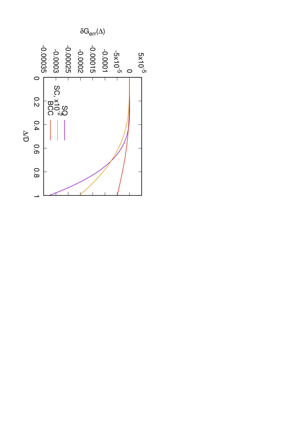
where primes stand for the derivative with respect to $\Delta$. The dependence of $G$ on $\Delta$ is fully determined by the spectrum $e_{-}(\mathbf{k})$ only, coinciding with full electron spectrum at $\tau=0$. Hence, the investigation of density of states for $e_{-}(\mathbf{k})$ allows to investigate in a convenient way analytical properties of $G(\Delta)$ and, through it, all other quantities. In the Appendix A we derive a general expansion of the lattice sum $G(\Delta)$ at small $\Delta$. For this purpose we recast Eq. (16) as

and from Eq. (12) we derive

A simple way of taking into account the local correlation effects on a qualitative level is to introduce the auxiliary slave boson states 1986:Kotliar; 1992:Fresard. This extends the configuration space of the Hamiltonian (5) to a bosonic sector by introducing the slave boson annihilation (creation) operators $e_{i}(e_{i}^{\dagger})$, $p_{i\sigma}(p_{i\sigma}^{\dagger}),d_{i}(d_{i}^{\dagger})$ for empty, singly and doubly occupied states, respectively. The transitions between the site states originating from intersite electron transfer are now accompanied by corresponding transitions in bosonic sector. The equivalence of the original and new description is achieved by the replacement $c_{i\sigma}\rightarrow\mathsf{z}_{i\sigma}c_{i\sigma}$, through a boson transfer operator $\mathsf{z}_{i\sigma}=(1-d^{\dagger}_{i}d_{i}-p^{\dagger}_{i\sigma}p_{i\sigma})^{-1/2}\left(e^{\dagger}_{i}p_{i\sigma}+p^{\dagger}_{i\bar{\sigma}}d_{i}\right)(1-e^{\dagger}_{i}e_{i}-p^{\dagger}_{i\bar{\sigma}}p_{i\bar{\sigma}})^{-1/2}$, which complements the action of $c_{i\sigma}$ on the bosonic subspace. The constraints

guarantee formal equivalence of SBA action to that of the original model.

This allows to recast exactly the interaction terms in the Hamiltonian (5) in the bosonic language

where $\tilde{\bf s}^{p}_{i}=(1/2)\sum_{\sigma\sigma^{\prime}}p^{\dagger}_{i\sigma}\vec{\sigma}_{\sigma\sigma^{\prime}}p_{i\sigma^{\prime}}$. Presence of the constraints can be taken into account within the functional integral formalism via the Lagrange multipliers [$\eta_{i}$ for Eq. (22), $\lambda_{i}$ for Eq. (23) and $\Delta_{i}$ for Eq. (24)] which are introduced into the action. Since we assume no any inhomogeneity, within the saddle-point approximation the operators $e_{i}(e^{\dagger}_{i}),p_{i\sigma}(p^{\dagger}_{i\sigma}),d_{i}(d^{\dagger}_{i})$ become $i$-independent slave boson amplitudes $e,p_{\sigma},d$, and $\mathsf{z}_{i\sigma}$ by $z_{\sigma}=(d^{2}+p_{\sigma}^{2})^{-1/2}(ep_{\sigma}+p_{\bar{\sigma}}d)(e^{2}+p_{\bar{\sigma}}^{2})^{-1/2}\leqslant 1$. The same argument holds for $\lambda_{i}$ and $\Delta_{i}$. Smallness of local electron spin-dependent quasiparticle residue $z_{\sigma}$ reflects the average incoherence of single and double states on a pair of sites between which a transfer occurs 2018:Igoshev. The difference of $z_{\uparrow}$ and $z_{\downarrow}$ residues can be induced by magnetic ordering away of half-filling. The grand potential $\Omega=-T\ln Z$, $T$ being the temperature, $Z$ being the partition function, can be presented as a sum of two contribution from fermion and boson subsystems, $\Omega^{\rm SBA}_{\rm AFM}=\Omega_{c}+\Omega_{b}$, where the fermion contribution to the grand potential

where $\mu$ is the chemical potential, is that of effective free-fermion Hamiltonian

which has AFM spectrum branches

where $\Delta(\mathbf{k})=\Delta-(z_{\uparrow}^{2}-z_{\downarrow}^{2})e_{+}(\mathbf{k})/2$.

The boson contribution to grand potential reads

From Eqs. (23) and (24) we get

which relates the electron filling $n$ and magnetization amplitude $m$ to boson amplitudes. Explicit equation determining slave boson parameters is given by general slave boson equations for the mean-field ansatz of slave boson amplitude and Lagrange multipliers (see, e.g., Ref. 2015:Igoshev). In the following we focus our attention on the case of insulator state at half-filling.

At half-filling ($n=1$), particle-hole symmetry results in the relations $e=d$, $z_{\uparrow}^{2}=z_{\downarrow}^{2}=z^{2}$, where

As a consequence, $\Delta(\mathbf{k})=\text{const}$, so that the subband spectrum acquires $\mathbf{k}$-independent narrowing. Here a slave boson amplitude correlation parameter $\zeta=2(p_{\uparrow}p_{\downarrow}-e^{2})$ indicates the difference of single and double electron state motion, which is neglected in the Hartree-Fock approximation. All the boson variables can be expressed through $m$ and $\zeta$, i.e.

thereby we fully exclude boson variables in the consideration below. Equation (33) yields the natural bound for $\zeta$: $\zeta<\zeta_{\rm max}=\sqrt{1-m^{2}}$. If $\zeta\lesssim\zeta_{\rm max}$, we have a strongly correlated regime with small quasiparticle weight, otherwise we are in the regime of a usual Fermi liquid.

For AFM insulator state, we assume that only lower subband ($\nu=1$) is filled, whereas upper one is empty. For this case, we call $z$ as $z_{\rm A}$ and $\zeta$ as $\zeta_{\rm A}$. Equations of Ref. 2015:Igoshev for the case of AFM insulator state can be strongly simplified:

with rescaled parameter $\Delta_{\ast}=\Delta/z^{2}_{\rm A}$. We see from Eq. (38) that the parameter $\Delta$ contains two terms: The first originates from intersite exchange and the second originates from local quantities (boson amplitudes).

From Eq. (37), it is clear that $m$ is a function of $\Delta_{\ast}$ only. We pass from $\Omega_{\rm AFM}^{\rm SBA}$ to the free energy $F_{\rm AFM}^{\rm SBA}=\Omega_{\rm AFM}^{\rm SBA}+\mu\cdot n$ at half-filling

The Eq. (39) imply $\zeta>0$, which imply positive definiteness of effective field $\Pi(\Delta_{\ast})=\Phi^{-1}_{1}(\Delta_{\ast})+J_{\mathbf{Q}}/(4z^{2}_{\rm A})>0$ from Eq. (38) $\Delta_{\ast}>\Delta_{J\ast}$, which gives with the use of Eq. (37) Introducing $\xi=\zeta_{\rm A}(2+\zeta_{\rm A})$, we solve Eq. (38) with respect to $\xi$ to obtain

Expanding $\Phi_{1}(\Delta_{\ast})$, $\Phi_{2}(\Delta_{\ast})$ and $\Pi(\Delta_{\ast})$ and, in turn, the Eq. (41) in powers of $\Delta_{\ast}$ allows to find expansions of all other quantities.

The Hartree-Fock approximation neglecting the difference between singly and doubly occupied states (see Sec. II.2) can be simply obtained in this way by replacing Eq. (38) by $\zeta=0$. Thereby $\zeta$ can be considered as a small parameter of the expansion and HFA is zero-order approximation of it. Here and below it is convenient to consider all quantities as functions of the rescaled gap $\Delta_{\ast}$. Analogously, introducing the definition $\delta F_{\rm AFM}^{\rm SBA}=F_{\rm AFM}^{\rm SBA}-F_{0}$ and picking up explicitly the HFA contribution given by Eq. (16) we get

Thus an improvement of HFA by correlation effects results not only in rescaling of AFM gap $\Delta\rightarrow\Delta_{\ast}$, but also in the occurrence of exchange (second) and correlation (third) terms, which both yield a manifestation of delicate many-electron effects.

In this section we consider free energy of the paramagnetic phase as a function of $\tau$ strictly at half-filling for all the considered bipartite (square, sc, and bcc) lattices. The peculiarity of the square lattice is the presence of persistent van Hove singularity in the electronic spectrum due to topological reason.

For bipartite lattices, at zero $\tau$ the Fermi level coincides with the van Hove singularity at the center of the band. The deviation of $\tau$ from zero shifts the van Hove singularity from the Fermi level, see Fig. 2.

For the paramagnetic phase we get within SBA (see Ref. 2015:Igoshev, $\zeta=\zeta_{\rm P}$, $z^{2}=z^{2}_{\rm P}$)

where $f[E]=(\exp[(E-\mu)/T]+1)^{-1}$ is the Fermi function and an PM phase analog of $\Phi_{2}$

The Fermi level $E_{\rm F}$ differs from $\mu$ by nonvaluable in a current context constant and is determined by Eq. (43) and the free energy of PM phase reads

As above, introducing the difference $\delta F_{\rm PM}^{\rm SBA}=F_{\rm PM}^{\rm SBA}-F_{0}$ we write down

where $\delta\Phi_{2\mathrm{P}}(\tau)=\Phi_{2\mathrm{P}}(\tau)-\Phi_{2}(0)$. We also directly obtain the analogous HFA expression by setting in the latter equation $\zeta_{\rm P}=0$, and $z_{\rm P}=1$ in Eq. (43),

It is clear that accounting the difference of single and double states within SBA, cf. Eqs. (48) and (49), allows to lower the energy of the paramagnetic state.

Vanishing of $e^{2}$ in Eq. (35) at $m=0$ means the condition of zero mobility of carriers, which yields in the paramagnetic phase critical $\zeta_{\rm P}=\zeta_{\rm BR}=1$ (the Brinkman-Rice realization of Mott scenario of metal-insulator transition), $\zeta_{\rm P}=\zeta$ in PM phase. Thus the transition to the metal state occurs at $U<U_{\rm BR}$ where

Direct calculations give $U^{\rm sq}_{\rm BR}=128/\pi^{2}=12.97$, $U^{\rm sc}_{\rm BR}=16.04$, $U^{\rm bcc}_{\rm BR}=16.51$.

To calculate the ground-state free energy of paramagnetic phase, see Eqs. (48) and (49), we use the explicit expressions for exact density of states at finite $\tau$ for the square, sc, and bcc lattices derived in Refs. 2019:Igoshev_JETP; 2019:Igoshev_FMM, where the presence of van Hove singularity lines at finite $\tau$ was found (at $\tau=0.25$ for sc lattice and $\tau=1.0$ for bcc lattice), which allows to solve Eqs. (43) and (44) numerically with extremely high precision.

For the square lattice, a finite $\tau$ value results in the shift of position of the van Hove singularity from $\varepsilon=0$: in Fig. 2a) the plots of density of states for the square lattice at different $\tau$ are shown. This dramatically distinguishes this case from three-dimensional cases [sc and bcc lattices, see Figs. 2b and 2c], where the deviation of $\tau$ from special values $\tau_{\ast}$ corresponding to topological transitions (for which the van Hove singularity line is present) results in destroying van Hove singularity lines (see details in Refs. 2019:Igoshev_FMM; 2019:Igoshev_JETP). For the square lattice at $\tau=0$ the Fermi level corresponding to half-filling coincides with the van Hove singularity position; at finite $\tau$ this is not the case, but the van Hove singularity holds its impact. For sc lattice the van Hove singularity is well away from zero, which results in an analytic dependence $E^{\rm sc}_{\rm F}$ on $\tau$; as a consequence one can see equidistant positions of the Fermi level at different $\tau$ with the same difference, see Fig. 2b). For bcc lattice, despite that van Hove singularity is absent at finite $\tau$, the peak below $\epsilon=E^{\rm bcc}_{\rm F}$ originates from heavy mass at the (saddle) van Hove point $\Lambda^{\ast}$ with large ($\propto\tau^{-1}$) three masses at the diagonal of the Brillouin zone, split off from P point as $\tau$ becomes nonzero. Nonequidistant positions of Fermi level can be seen even by eye for both square and bcc lattices, see Figs. 2a and 2c. We can therefore state that heavy mass of diagonal (saddle) van Hove singularity point enhancement holds its impact on thermodynamic quantities, e.g., the free energy, which indicates the similarity of the bcc and square lattices. In Fig. 3 the dependence of $E_{\rm F}/\tau$ in the PM phase as a function of $\tau$ is shown for the square, sc and bcc lattices. For the square and bcc lattices the dependence of $E_{\rm F}$ on $\tau$ is nonanalytical in the vicinity of $\tau=0$, and the van Hove DOS singularity for bcc lattice present at $\tau=0$ retains to great extent its impact on the Fermi energy due to strong mass enhancement at $\Lambda^{\ast}$ point, see Refs. 2019:Igoshev_FMM; 2019:Igoshev_JETP.

In this subsection we present the results of numerical analysis of the sign of expression (56) for different lattices and approximation used. In Fig. 5 the free energies of AFM insulator and PM metal phases on MIT line, Eq. (51), within both HFA (see the Sec. II.2) and SBA (see Sec. II.4) are shown. Whereas for the square lattice the free energies of AFM and PM phases are found to be very close (especially within the HFA), for sc and especially for bcc (due to lowering of the free energy of AFM phase caused by vHS of DOS at $\tau=0$) lattices, the energy of AFM insulator phase is considerably lower than the energy of PM metal phase in both the approximations used. We find that correlation effects considerably reduce the energy of both phases $\delta F_{\rm AFM}$ and $\delta F_{\rm PM}$ at MIT line. However, this reducing is substantially stronger for paramagnetic phase. Another correlation effect is the occurrence of nonanalytic contributions $\sim\zeta^{2}$ (as a function of $\tau$) to the free energy, see Eq. (39), which yields considerable contribution at small $\tau$ [see Fig. 5b]. From Eqs. (39) and (44) we see that at small $\tau$ $\zeta_{\rm A}\sim\zeta_{\rm P}\sim 2/(\Phi_{1}(\Delta_{\rm MIT}(\tau))U_{\rm BR})$, therefore the nonanalytic behaviour of $\zeta_{\rm P,A}$ is determined by that of $\Phi_{1}$, which is very different for different lattices, see derivation in the Appendix A.

In all the cases the correlation effects increase $\Delta F_{\rm MIT}$, which enhances the tendency towards first-order MIT. In Fig. 6 the free energy difference $\Delta F_{\rm MIT}(\tau)$ on the MIT line (51), see Eq. (56), is shown for the square, sc and bcc lattices. We find that whereas for considered three-dimensional lattices $\Delta F_{\rm MIT}(\tau)<0$, for the square lattice the sign change of $\Delta F_{\rm MIT}(\tau)$ occurs at small $\tau$ since the free energies of AFM and PM phases are still very close, so that an accurate consideration is needed in both HFA and SBA approximation.

In the following subsections we analyze the impact of correlations and exchange interaction effects on the PM–AFM insulator free energy difference on the hypothetical MIT line within AFM phase (see Sec. III.2) and derive an expansion of the free-energy of AFM insulator phase for the square lattice to reveal the origin for smallness of free energy difference found above, see also Refs. 2000:Yang; 2010:Yu (also see Sec. III.3).

Here we analyze the contributions of correlations and exchange intersite interactions into $\Delta F_{\rm MIT}$ on the MIT line within AFM phase. Since both these contributions are pure correlation effects beyond HFA and are of fourth order with respect to $\tau$, it can be expected that they start to play role with increasing $\tau$.

Since the exchange interaction enters all equation through its Fourier transform, for simplicity we use the approximation for exchange integrals: $J_{\mathbf{Q}}=-Z_{\rm nn}J$, $J(Z_{\rm nn})$ being the nearest-neighbor exchange integral (number). In Fig. 7a we show $\Delta F_{\rm MIT}$ on the MIT line in the presence of exchange interaction of different sign. It is worthwhile to note that the main part of the interaction is absorbed into the gap and does not affect $\Delta F_{\rm MIT}$, but only its subleading part plays a role. This subleading contribution is inaccessible within HFA and has a delicate many-electron nature.

Applying the method considered above to the case of finite exchange interaction we find that $\Delta F_{\rm MIT}$ is rather sensitive to the value of $J$: positive (negative) $J$ results in decreasing (increasing) of $\Delta F_{\rm MIT}$. Thus, we may expect an intersite exchange interaction can change the MIT order transition, which is purely many-electron effect. Figure 7b provides the phase diagram in terms of $J-\tau_{\rm c}$, where $\tau_{\rm c}$ is determined by the equation $\Delta F_{\rm MIT}\left(\Delta_{\rm MIT}(\tau),J\right)=0$ and is actually the critical $\tau$ separating the first- and second-order transition regions. One can see that the exchange interaction of “ferromagnetic” sign $J<0$ can transform the second-order transition into the first-order one reducing the stripe of AFM metal in the phase diagrams (see Fig. 1): For the square lattice the change of exchange integral shifts $\tau$ point of MIT order change only weakly, whereas for sc and bcc lattices substantially large values of exchange integral are needed for the change. Also we note that the sensitivity of $\Delta F_{\rm MIT}$ with respect to $J$ value is very different for different lattices: the size of the effect is determined by DOS van Hove singularity at $\tau=0$. Note that the results for MIT line in Fig. 7b for sc and bcc lattices should be considered with a caution, since at large $\tau\sim 0.5$ other (spiral) phases with lower free energy may occur destroying the two-sublattice antiferromagnetic order 2016:Timirgazin. At the same time, the results for small $\tau$ seem to be reliable.

Now we analyze different contributions in $\Delta F_{\rm MIT}(\Delta_{\ast})$ to trace explicitly the influence of many-electron effects and exchange interaction on the order of MIT. From Eqs. (42) and (48) we have

We exclude $\zeta_{\rm A,P}$ using Eqs. (39) and (44),

where $\alpha_{\rm A}=\delta\Phi_{2}(\Delta_{\ast})/\Phi_{2}(0)$, $\alpha_{\rm P}=\delta\Phi_{2\rm P}\left(\tau_{\rm MIT}(\Delta_{\ast})\right)/\Phi_{2}(0)$ and the dimensionless interaction parameter

is introduced.

We split the expression (57)

where

where

References

• (1) M.Imada, A. Fujimori, Y. Tokura, Rev. Mod. Phys. 70, 1039 (1998)
• (2) F. Gebhard. The Mott Metal-Insulator Transition: Models and Methods, – Springer. Berlin–Heidelberg (1997).
• (3) N.F. Mott, Metal-Insulator Transitions, Taylor & Francis Ltd. (1974).
• (4) M. Schuler, E.G.C.P. van Loon, M.I. Katsnelson, and T.O. Wehling, Phys. Rev. B 97, 165135 (2018).
• (5) J.C.Slater, Phys. Rev. 51, 538 (1951).
• (6) N.F. Mott, Proc. Phys. Soc. London, Ser. A 62, 416 (1949).
• (7) Y.G. Shi, Y.F. Guo, S. Yu, M. Arai, A.A. Belik, A. Sato, K. Yamaura, E. Takayama-Muromachi, H.F. Tian, H.X. Yang, J. Q. Li, T. Varga, J. F. Mitchell, and S. Okamoto, Phys. Rev. B 80, 161104(R) (2009).
• (8) S. Calder, V.O. Garlea, D.F. McMorrow, M.D. Lumsden, M.B. Stone, J.C. Lang, J.W. Kim, J.A. Schlueter, Y.G. Shi, K. Yamaura, Y.S. Sun, Y. Tsujimoto, and A.D. Christianson, Phys. Rev. Lett. 108, 257209 (2012).
• (9) M.-C. Jung, Y.-J. Song, K.-W. Lee, and W. E. Pickett, Phys. Rev. B 87, 115119 (2013).
• (10) K. Matsuhira, M. Wakeshima, Y. Hinatsu, and S. Takagi, J. Phys. Soc. Jpn. 80, 094701 (2011).
• (11) D. Mandrus, J.R. Thompson, R. Gaal, L. Forro, J.C. Bryan, B.C. Chakoumakos, L.M. Woods, B.C. Sales, R. S. Fishman, and V. Keppens, Phys. Rev. B 63, 195104 (2001).
• (12) H. Jacobsen, H.L. Feng, A.J. Princep, M.C. Rahn, Y. Guo, J. Chen, Y. Matsushita, Y. Tsujimoto, M. Nagao, D. Khalyavin, P. Manuel, C.A. Murray, Ch. Donnerer, J.G. Vale, M.M. Sala, K. Yamaura, A.T. Boothroyd, Phys. Rev. B 102, 214409 (2020).
• (13) J. Trastoy, A. Camjayi, J. del Valle, Y. Kalcheim, J.-P. Crocombette, D.A. Gilbert, J.A. Borchers, J.E. Villegas, D. Ravelosona, M.J. Rozenberg, and I.K. Schuller, Phys. Rev. B 101, 245109 (2020).
• (14) S. A. Carter, T. F. Rosenbaum, J. M. Honig, and J. Spalek, Phys. Rev. Lett. 67, 3440 (1991).
• (15) S. Sudo, J. Magn. Mag. Mat. 114, 57 (1992).
• (16) B. Xu, P. Marsik, E. Sheveleva, F. Lyzwa, A. Louat, V. Brouet, D. Munzar, and C. Bernhard, Phys. Rev. Lett. 124, 027402 (2020).
• (17) J. Hubbard, Proc. Roy. Soc. Series A. 276, 238 (1963).
• (18) J. Hubbard, Proc. Roy. Soc. Series A. 281, 401 (1964)
• (19) M.I. Katsnelson and V.Yu. Irkhin, J. Phys. C 17, 4291 (1984).
• (20) P. Korbel, W. Wójcik, A. Klejnberg et al., Eur. Phys. J. B 32, 315 (2003).
• (21) M. Salmhofer and C. Honerkamp, Prog. Theor. Phys. 105, 1 (2001).
• (22) C. Honerkamp and M. Salmhofer, Phys. Rev. B 64, 184516 (2001).
• (23) H. J. Schulz, Phys. Rev. Lett. 64, 1445 (1990).
• (24) P.A. Igoshev, M.A. Timirgazin, V.F. Gilmutdinov, A.K. Arzhnikov and V. Yu. Irkhin, J. Phys.: Cond. Matt. 27, 446002 (2015).
• (25) P.A. Igoshev, A.A. Katanin, V.Yu. Irkhin, JETP 105, 1043 (2007).
• (26) P.A. Igoshev, M.A. Timirgazin, A.A. Katanin, A.K. Arzhnikov and V.Yu. Irkhin, Phys. Rev. B 81, 094407 (2010).
• (27) P.A. Igoshev, V.Yu. Irkhin, and A.A. Katanin, Phys. Rev. B 83, 245118 (2011).
• (28) T. Das, R.S. Markiewicz, and A. Bansil, Adv. Phys. 63, 151 (2014).
• (29) W. Hofstetter and D. Vollhardt, Ann. Phys. 7, 48 (1998).
• (30) P.A. Igoshev, V.Yu. Irkhin, JETP 128, 909 (2019).
• (31) T. Misawa and M. Imada, Phys. Rev. B 75, 115121 (2007).
• (32) R. Chitra and G. Kotliar, Phys. Rev. Lett. 83, 2386 (1999).
• (33) M. A. Timirgazin, P. A. Igoshev, A. K. Arzhnikov, V. Yu. Irkhin, J. Low. Temp. Phys. 185, 651 (2016).
• (34) H. Kondo and T. Moriya, J. Phys. Soc. Jpn. 65, 2559 (1996).
• (35) D. Duffy and A. Moreo, Phys. Rev. B 55, R676 (1997).
• (36) Z.-Q. Yu and L. Yin, Phys. Rev. B 81, 195122 (2010).
• (37) P.A. Igoshev, V.Yu. Irkhin, Physics of Metals and Metallography 120, 1282 (2019).
• (38) P.A. Igoshev, V.Yu. Irkhin, JETP Letters 110, 727 (2019).
• (39) L. van Hove, Phys. Rev. 89, 1189 (1953).
• (40) H. Q. Lin and J. E. Hirsch, Phys. Rev. B 35, 3359 (1987).
• (41) A. Yamada, K. Seki, R. Eder, and Y. Ohta Phys. Rev. B 88, 075114 (2013).
• (42) A.H. Nevidomskyy, C. Scheiber, D. Senechal, and A. M. S. Tremblay, Phys. Rev. B 77, 064427 (2008).
• (43) H. Yokoyama, M. Ogata and Y. Tanaka, J. Phys. Soc. Jpn. 75, 114706 (2006).
• (44) F. Becca, L.F. Tocchio, and S. Sorella, Journal of Physics: Conference Series 145, 012016 (2009).
• (45) L.F. Tocchio, F. Becca, A. Parola, and S. Sorella Phys. Rev. B 78, 041101(R) (2008).
• (46) T. Kashima and M. Imada, J. Phys. Soc. Jpn. 70, 3052 (2001).
• (47) H. Morita, S. Watanabe, and M. Imada, J. Phys. Soc. Jpn. 71, 2109 (2002).
• (48) T. Mizusaki, and M. Imada, Phys. Rev. B 74, 014421 (2006).
• (49) G. Kotliar and A.E. Ruckenstein, Phys. Rev. Lett. 57, 1362 (1986).
• (50) I. Yang, E. Lange, and G. Kotliar, Phys. Rev. B 61, 2521 (2000).
• (51) Th. Pruschke and R. Zitzler, J. Phys.: Condens. Matter 15, 7867 (2003).
• (52) R. Zitzler, N.-H. Tong, Th. Pruschke, and R. Bulla, Phys. Rev. Lett. 93, 016406 (2004).
• (53) R. Peters and Th. Pruschke, Phys. Rev. B 79, 045108 (2009).
• (54) L. Fratino, M. Charlebois, P. Semon, G. Sordi, and A. M. S. Tremblay, Phys. Rev. B 96, 241109(R) (2017).
• (55) M. Eckstein, M. Kollar, M. Potthoff, and D. Vollhardt, Phys. Rev. B 75, 125103 (2007).
• (56) R. Fresard and P. Wölfle, J. Phys.: Cond. Matt. 4, 3625 (1992).
• (57) P.A. Igoshev, M.A. Timirgazin, A.K. Arzhnikov, V.Yu. Irkhin, J. of Magn. and Magn. Materials 459, 311 (2018).
• (58) M. A. Timirgazin, P. A. Igoshev, A. K. Arzhnikov, V. Yu. Irkhin, J. Phys.: Cond. Matt. 28, 505601 (2016).
Appendix A Expansion of G⁡(Δ)G(\Delta) at small Δ\Delta
We consider the expansion of Eq. (17) of the main text in powers of Δ\Delta, which can be presented through the density of states of the spectrum at τ=0\tau=0, ρ⁡(ε)≡ρ⁡(ε,τ=0)\rho(\varepsilon)\equiv\rho(\varepsilon,\tau=0)
G⁡(Δ)=∫0+Dd​ε​ρ​(ε)|ε|+Δ2+ε2,G(\Delta)=\int_{0}^{+D}\frac{d\varepsilon\,\rho(\varepsilon)}{|\varepsilon|+\sqrt{\Delta^{2}+\varepsilon^{2}}}, (95)
where the parity of ρ⁡(ε)\rho(\varepsilon) for bipartite lattice is taken into account. Since direct setting Δ=0\Delta=0 results in diverging integrals, we conclude that the parameter Δ\Delta cuts the divergence, and leading terms are determined by the contributions of small ε\varepsilon. We take DD as an energy unit, ϵ=ε/D,d=Δ/D\epsilon=\varepsilon/D,d=\Delta/D, up to the end of the Appendix: G⁡(Δ)=D−1​𝒢​(Δ/D)G(\Delta)=D^{-1}\mathcal{G}(\Delta/D), where
𝒢⁡(d)=∫0+1d​ϵ​ρD​(ϵ)ϵ+d2+ϵ2,\mathcal{G}(d)=\int_{0}^{+1}\frac{d\epsilon\,\rho_{D}(\epsilon)}{\epsilon+\sqrt{d^{2}+\epsilon^{2}}}, (96)
where ρD​(ϵ)=D​ρ​(D​ϵ)\rho_{D}(\epsilon)=D\rho(D\epsilon) is rescaled density of states.
We can introduce a “logarithmic index” nln_{\rm l} for a lattice as a maximal power of logarithms entering the expansion of the DOS in the vicinity of ε=0\varepsilon=0. We consider three cases of the DOS behaviour at small ε\varepsilon: (i) double-logarithmic behaviour, nl=2n_{\rm l}=2 (an example is bcc lattice), (ii) logarithmic behaviour, nl=1n_{\rm l}=1 (an example is square lattice), (iii) regular (analytic) behaviour, nl=0n_{\rm l}=0 (an example is sc lattice) 1969:Jelitto. As we will see below, all these case are captured by the following general representation:
𝒢⁡(d)=∑n=0nl+1an​lnn​2d+d2​∑n=0nl+1bn​lnn​2d+𝒪⁡(d4​lnnl+1​2d),\mathcal{G}(d)=\sum_{n=0}^{n_{\rm l}+1}a_{n}\ln^{n}\frac{2}{d}+d^{2}\sum_{n=0}^{n_{\rm l}+1}b_{n}\ln^{n}\frac{2}{d}+\mathcal{O}\left(d^{4}\ln^{n_{\rm l}+1}\frac{2}{d}\right), (97)
where the coefficients an,bna_{n},b_{n} are specified by a concrete lattice.
From the representations (18),(19), and asymptotic form (97) we get the expansions
Φ1​(d⋅D)=2D​(∑n=0nl+1(2​an−(n+1)​an+1)​lnn​2d+d2​∑n=0nl+1(4​bn−(n+1)​bn+1)​lnn​2d)+𝒪⁡(d4​lnnl+1​2d),\Phi_{1}(d\cdot D)=\frac{2}{D}\left(\sum_{n=0}^{n_{\rm l}+1}(2a_{n}-(n+1)a_{n+1})\ln^{n}\frac{2}{d}\\ +d^{2}\sum_{n=0}^{n_{\rm l}+1}\left(4b_{n}-(n+1)b_{n+1}\right)\ln^{n}\frac{2}{d}\right)+\mathcal{O}\left(d^{4}\ln^{n_{\rm l}+1}\frac{2}{d}\right), (98)
δ​Φ2​(d⋅D)=−2​D​(d2​∑n=0nl+1(an−(n+1)​an+1)​lnn​2d+d4​∑n=0nl+1(3​bn−(n+1)​bn+1)​lnn​2d)+𝒪⁡(d6​lnnl+1​2d),\delta\Phi_{2}(d\cdot D)=-2D\left(d^{2}\sum_{n=0}^{n_{\rm l}+1}(a_{n}-(n+1)a_{n+1})\ln^{n}\frac{2}{d}\\ +d^{4}\sum_{n=0}^{n_{\rm l}+1}\left(3b_{n}-(n+1)b_{n+1}\right)\ln^{n}\frac{2}{d}\right)+\mathcal{O}\left(d^{6}\ln^{n_{\rm l}+1}\frac{2}{d}\right), (99)
where we define anl+2=bnl+2=0a_{n_{\rm l}+2}=b_{n_{\rm l}+2}=0. From Eq. (20) and asymptotic form (97) we obtain the asymptotics of HFA free energy
δ​FAFMHFA​(d⋅D)=−D⁡(d2​∑n=0nl(n+1)​an+1​lnn​2d+d4​∑n=0nl+1((n+1)​bn+1−2​bn)​lnn​2d+𝒪⁡(d6​lnnl+1​2d)).\delta F^{\rm HFA}_{\rm AFM}(d\cdot D)=-D\left(d^{2}\sum_{n=0}^{n_{\rm l}}(n+1)a_{n+1}\ln^{n}\frac{2}{d}+d^{4}\sum_{n=0}^{n_{\rm l}+1}((n+1)b_{n+1}-2b_{n})\ln^{n}\frac{2}{d}+\mathcal{O}\left(d^{6}\ln^{n_{\rm l}+1}\frac{2}{d}\right)\right). (100)
We see that the expansion of free energy of AFM insulator state always contains singular contributions, but their role dramatically depends on the presence of singularity of DOS at τ=0\tau=0: if ρ⁡(ϵ)\rho(\epsilon) is analytic in the vicinity of ϵ=0\epsilon=0, non-analytic contribution enters starting from subleading terms, whereas for singular ρ⁡(ϵ)\rho(\epsilon) already the leading contribution is singular.
Since at small dd main contribution originates from small ϵ\epsilon, we separate from the ρD​(ϵ)\rho_{D}(\epsilon), which is an even function of ϵ\epsilon, the leading contribution in the vicinity of ϵ=0\epsilon=0:
ρD​(ϵ)=ρD,s​(ϵ)+ρD,quad​(ϵ)+δ​ρD​(ϵ),\rho_{D}(\epsilon)=\rho_{D,\rm s}(\epsilon)+\rho_{D,\rm quad}(\epsilon)+\delta\rho_{D}(\epsilon), (101)
where ρD,s​(ϵ)\rho_{D,\rm s}(\epsilon) is leading (double-logarithmic, logarithmic or constant contribution), ρD,quad​(ϵ)\rho_{D,\rm quad}(\epsilon) is subleading contribution ∼ϵ2​lnnl⁡(1/ϵ)\sim\epsilon^{2}\ln^{n_{\rm l}}(1/\epsilon), and δ​ρ​(ϵ)∼ϵ4​lnnl⁡(1/ϵ)\delta\rho(\epsilon)\sim\epsilon^{4}\ln^{n_{\rm l}}(1/\epsilon) is rest contribution which therefore yields only small corrections.
A.1 Asymptotics for 𝒢⁡(d)\mathcal{G}(d)
Here we derive a general asymptotics for 𝒢⁡(d)\mathcal{G}(d) for different forms of the density of states up to d2​lnnl+1​1dd^{2}\ln^{n_{\rm l}+1}\frac{1}{d}. We determine the singular contributions at d→0d\rightarrow 0 and regular contributions up to o⁡(d)o(d): 𝒢⁡(d)=𝒢s​(d)+𝒢quad​(d)+δ​𝒢​(d)\mathcal{G}(d)=\mathcal{G}_{\rm s}(d)+\mathcal{G}_{\rm quad}(d)+\delta\mathcal{G}(d), where
(𝒢s​(d)𝒢quad​(d)δ​𝒢​(d))=∫01(ρD,s​(ϵ)ρD,quad​(ϵ)δ​ρD​(ϵ))​d​ϵϵ2+d2+ϵ.\begin{pmatrix}\mathcal{G}_{\text{s}}(d)\\ \mathcal{G}_{\text{quad}}(d)\\ \delta\mathcal{G}(d)\end{pmatrix}=\int\limits_{0}^{1}\begin{pmatrix}\rho_{D,\rm s}(\epsilon)\\ \rho_{D,\rm quad}(\epsilon)\\ \delta\rho_{D}(\epsilon)\end{pmatrix}\frac{d\epsilon}{\sqrt{\epsilon^{2}+d^{2}}+\epsilon}. (102)
Below we use the identity
∫01dxlnn⁡(1/x)x+a=−n!Lin+1(−1/a),a>0,\int\limits_{0}^{1}dx\,\frac{\ln^{n}(1/x)}{x+a}=-n!\text{Li}_{n+1}(-1/a),\;a>0, (103)
where Lin\text{Li}_{n} is polylogarithm function. An idea of derivation of an asymptotic integrals is to choose a simple function having a similar behaviour of the integrand in the regions giving main contribution to the integral: ϵ≪d\epsilon\ll d and ϵ≫d\epsilon\gg d:
ϵ2+d2+ϵ→2​ϵ+d.\sqrt{\epsilon^{2}+d^{2}}+\epsilon\rightarrow 2\epsilon+d. (104)
We investigate the contribution of double-logarithmic singularity (dl)ρD,s​(ϵ)=ln2⁡(1/ϵ)\rho_{D,\rm s}(\epsilon)=\ln^{2}(1/\epsilon):
𝒢dl(d)≡∫01dϵln2⁡(1/ϵ)ϵ2+d2+ϵ→𝒢¯dl(d)≡∫01dϵln2⁡(1/ϵ)2​ϵ+d=−Li3(−2/d).\mathcal{G}_{\rm dl}(d)\equiv\int\limits_{0}^{1}d\epsilon\,\frac{\ln^{2}\left(1/\epsilon\right)}{\sqrt{\epsilon^{2}+d^{2}}+\epsilon}\rightarrow\bar{\mathcal{G}}_{\rm dl}(d)\equiv\int\limits_{0}^{1}d\epsilon\,\frac{\ln^{2}\left(1/\epsilon\right)}{2\epsilon+d}=-\mathrm{Li}_{3}(-2/d). (105)
Using Eq. (103) and expanding Li3(−2/d)\mathrm{Li}_{3}(-2/d) at small dd we obtain
𝒢¯dl​(d)=16​(ln3⁡2d+π2​ln⁡2d)+d/2−d2/32+o⁡(d2).\bar{\mathcal{G}}_{\rm dl}(d)=\frac{1}{6}\left(\ln^{3}\frac{2}{d}+\pi^{2}\ln\frac{2}{d}\right)+d/2-d^{2}/32+o(d^{2}). (106)
Introducing the variable change x=ϵ/dx=\epsilon/d we write the difference of 𝒢dl​(d)\mathcal{G}_{\rm dl}(d) and 𝒢¯dl​(d)\bar{\mathcal{G}}_{\rm dl}(d) as
𝒢dl​(d)−𝒢¯dl​(d)=∫01/dd​x​ln2​1x​d​(1x2+1+x−12​x+1).\mathcal{G}_{\rm dl}(d)-\bar{\mathcal{G}}_{\rm dl}(d)=\int\limits_{0}^{1/d}dx\,\ln^{2}\frac{1}{xd}\left(\frac{1}{\sqrt{x^{2}+1}+x}-\frac{1}{2x+1}\right). (107)
Extending the upper integral limit to infinity
∫0+∞d​x​ln2​1x​d​(1x2+1+x−12​x+1)=14​(ln2⁡2d+(1−π23)​ln⁡2d+(12+ζ⁡(3)+π26))\int\limits_{0}^{+\infty}dx\,\ln^{2}\frac{1}{xd}\left(\frac{1}{\sqrt{x^{2}+1}+x}-\frac{1}{2x+1}\right)=\frac{1}{4}\left(\ln^{2}\frac{2}{d}+\left(1-\frac{\pi^{2}}{3}\right)\ln\frac{2}{d}+\left(\frac{1}{2}+\zeta(3)+\frac{\pi^{2}}{6}\right)\right) (108)
and estimating an error introduced thereby,
∫1/d∞d​x​ln2​1x​d​(1x2+1+x−12​x+1)=∫1/d∞d​x​(1−1/x+…)4​x2​ln2​1x​d=d⁡(1−d/8)2+o⁡(d2),\int\limits_{1/d}^{\infty}dx\,\ln^{2}\frac{1}{xd}\left(\frac{1}{\sqrt{x^{2}+1}+x}-\frac{1}{2x+1}\right)=\int\limits_{1/d}^{\infty}\frac{dx(1-1/x+\ldots)}{4x^{2}}\,\ln^{2}\frac{1}{xd}=\frac{d(1-d/8)}{2}+o(d^{2}), (109)
we have the result
𝒢dl​(d)−𝒢¯dl​(d)=14​(ln2⁡2d+(1−π23)​ln⁡2d+(12+ζ⁡(3)+π26))−d⁡(1−d/8)2+o⁡(d2).\mathcal{G}_{\rm dl}(d)-\bar{\mathcal{G}}_{\rm dl}(d)=\frac{1}{4}\left(\ln^{2}\frac{2}{d}+\left(1-\frac{\pi^{2}}{3}\right)\ln\frac{2}{d}+\left(\frac{1}{2}+\zeta(3)+\frac{\pi^{2}}{6}\right)\right)-\frac{d(1-d/8)}{2}+o(d^{2}). (110)
Summing the expressions (106) and (110) we get
𝒢dl​(d)=16​(ln3⁡2d+32​ln2​2d+12​(π2+3)​ln⁡2d+32​(12+ζ⁡(3)+π26))+d2/32+o⁡(d2).\mathcal{G}_{\rm dl}(d)=\frac{1}{6}\left(\ln^{3}\frac{2}{d}+\frac{3}{2}\ln^{2}\frac{2}{d}+\frac{1}{2}\left(\pi^{2}+3\right)\ln\frac{2}{d}+\frac{3}{2}\left(\frac{1}{2}+\zeta(3)+\frac{\pi^{2}}{6}\right)\right)+d^{2}/32+o(d^{2}). (111)
Now we consider the contribution from the logarithmic (l) singularity ρD,s​(ϵ)=ln⁡(1/ϵ)\rho_{D,\rm s}(\epsilon)=\ln(1/\epsilon):
𝒢l(d)=∫01dϵln⁡(1/ϵ)ϵ2+d2+ϵ→𝒢¯l(d)=∫01dϵln⁡(1/ϵ)2​ϵ+d=−12Li2(−2/d).\mathcal{G}_{\rm l}(d)=\int\limits_{0}^{1}d\epsilon\,\frac{\ln\left(1/\epsilon\right)}{\sqrt{\epsilon^{2}+d^{2}}+\epsilon}\rightarrow\bar{\mathcal{G}}_{\rm l}(d)=\int\limits_{0}^{1}d\epsilon\,\frac{\ln\left(1/\epsilon\right)}{2\epsilon+d}=-\frac{1}{2}\text{Li}_{2}(-2/d). (112)
From Eq. (103) we obtain the asymptotics
𝒢¯l​(d)=14​ln2​2d+π212−d/4+d2/32+o⁡(d).\bar{\mathcal{G}}_{\rm l}(d)=\frac{1}{4}\ln^{2}\frac{2}{d}+\frac{\pi^{2}}{12}-d/4+d^{2}/32+o(d). (113)
As above, we introduce the variable change x=ϵ/dx=\epsilon/d to obtain
𝒢l​(d)−𝒢¯l​(d)=∫01/dd​x​ln⁡1x​d​(1x2+1+x−12​x+1).\mathcal{G}_{\rm l}(d)-\bar{\mathcal{G}}_{\rm l}(d)=\int\limits_{0}^{1/d}dx\,\ln\frac{1}{xd}\left(\frac{1}{\sqrt{x^{2}+1}+x}-\frac{1}{2x+1}\right). (114)
Similar to above consideration, we extend the upper limit to infinity,
∫0+∞d​x​ln⁡1x​d​(1x2+1+x−12​x+1)=14​(ln⁡2d+3−π26)\int\limits_{0}^{+\infty}dx\,\ln\frac{1}{xd}\left(\frac{1}{\sqrt{x^{2}+1}+x}-\frac{1}{2x+1}\right)=\frac{1}{4}\left(\ln\frac{2}{d}+\frac{3-\pi^{2}}{6}\right) (115)
and
∫1/d∞d​x​ln⁡1x​d​(1x2+1+x−12​x+1)=∫1/d∞d​x​(1−1/x+…)4​x2​ln2​1x​d=−d4​(1−d/4)+o⁡(d2)\int\limits_{1/d}^{\infty}dx\,\ln\frac{1}{xd}\left(\frac{1}{\sqrt{x^{2}+1}+x}-\frac{1}{2x+1}\right)=\int\limits_{1/d}^{\infty}\frac{dx(1-1/x+\ldots)}{4x^{2}}\,\ln^{2}\frac{1}{xd}=-\frac{d}{4}(1-d/4)+o(d^{2}) (116)
𝒢l​(d)−𝒢¯l​(d)=14​(ln⁡2d+3−π26)+d4​(1−d/4)+o⁡(d2).\mathcal{G}_{\rm l}(d)-\bar{\mathcal{G}}_{\rm l}(d)=\frac{1}{4}\left(\ln\frac{2}{d}+\frac{3-\pi^{2}}{6}\right)+\frac{d}{4}(1-d/4)+o(d^{2}). (117)
Summing both the contributions (113) and (117), we obtain
𝒢l​(d)=14​(ln2⁡2d+ln⁡2d+3+π26)−d2/32+o⁡(d2).\mathcal{G}_{\rm l}(d)=\frac{1}{4}\left(\ln^{2}\frac{2}{d}+\ln\frac{2}{d}+\frac{3+\pi^{2}}{6}\right)-d^{2}/32+o(d^{2}). (118)
The contribution from ρD​(ϵ)=1\rho_{D}(\epsilon)=1 is
𝒢0​(d)=12​(12+ln⁡2d)+d2/16+o⁡(d2).\mathcal{G}_{0}(d)=\frac{1}{2}\left(\frac{1}{2}+\ln\frac{2}{d}\right)+d^{2}/16+o(d^{2}). (119)
Now we consider the contribution from quadratic (possibly with logarithmic corrections) term in the density of state ρD;quad​(ϵ)=ϵ2\rho_{D;\rm quad}(\epsilon)=\epsilon^{2}:
𝒢quad​(d)=∫01d​ϵ​ϵ2ϵ2+d2+ϵ=14−d232​(4​ln⁡2d−1)+o⁡(d3),\mathcal{G}_{\rm quad}(d)=\int\limits_{0}^{1}d\epsilon\,\frac{\epsilon^{2}}{\sqrt{\epsilon^{2}+d^{2}}+\epsilon}=\frac{1}{4}-\frac{d^{2}}{32}\left(4\ln\frac{2}{d}-1\right)+o(d^{3}), (120)
and for ρD;quad,l​(ϵ)=ϵ2​ln⁡(1/|ϵ|)\rho_{D;\rm quad,l}(\epsilon)=\epsilon^{2}\ln(1/|\epsilon|)
𝒢quad,l​(d)=∫01d​ϵ​ϵ2​ln⁡(1/ϵ)ϵ2+d2+ϵ=18−d216​(ln2⁡2d−12​ln⁡2d+4​π2−1524)+o⁡(d3).\mathcal{G}_{\rm quad,l}(d)=\int\limits_{0}^{1}d\epsilon\,\frac{\epsilon^{2}\ln(1/\epsilon)}{\sqrt{\epsilon^{2}+d^{2}}+\epsilon}=\frac{1}{8}-\frac{d^{2}}{16}\left(\ln^{2}\frac{2}{d}-\frac{1}{2}\ln\frac{2}{d}+\frac{4\pi^{2}-15}{24}\right)+o(d^{3}). (121)
For ρD;quad,2​l​(ϵ)=ϵ2​ln2⁡(1/|ϵ|)\rho_{D;\rm quad,2l}(\epsilon)=\epsilon^{2}\ln^{2}(1/|\epsilon|)
𝒢quad,dl​(d)=∫01d​ϵ​ϵ2​ln2⁡(1/ϵ)ϵ2+d2+ϵ=18−d2​∑n=03gnquad,2​l​lnn​2d+o⁡(d3),\mathcal{G}_{\rm quad,dl}(d)=\int\limits_{0}^{1}d\epsilon\,\frac{\epsilon^{2}\ln^{2}(1/\epsilon)}{\sqrt{\epsilon^{2}+d^{2}}+\epsilon}=\frac{1}{8}-d^{2}\sum_{n=0}^{3}g^{\rm quad,2l}_{n}\ln^{n}\frac{2}{d}+o(d^{3}), (122)
where g0quad,2​l=(48​ζ​(3)−4​π2−39)/768g^{\rm quad,2l}_{0}=\left(48\zeta(3)-4\pi^{2}-39\right)/{768}, g1quad,2​l=(4​π2−15)/192g^{\rm quad,2l}_{1}=(4\pi^{2}-15)/{192}, gquad,2​l2=−1/32g^{\rm quad,2l}_{2}=-1/{32}, g3quad,2​l=1/24g^{\rm quad,2l}_{3}=1/{24}.
Finally, we take into account the contribution δ​𝒢​(d)\delta\mathcal{G}(d) from the rest part of the density of states presenting ρD​(ϵ)=ρD,leading​(ϵ)+δ​ρD​(ϵ)\rho_{D}(\epsilon)=\rho_{D,\rm leading}(\epsilon)+\delta\rho_{D}(\epsilon), where ρD,leading​(ϵ)\rho_{D,\rm leading}(\epsilon) is some linear combination of the above-considered logarithmic and quadratic contributions, and δ​ρD​(ϵ)=o⁡(ϵ3)\delta\rho_{D}(\epsilon)=o(\epsilon^{3}). Since the integral ∫01d​ϵ​δ​ρD​(ϵ)/ϵ3\int\limits_{0}^{1}\,d\epsilon\delta\rho_{D}(\epsilon)/\epsilon^{3} converges, we apply the expansion for the contribution of δD​ρ​(ϵ)\delta_{D}\rho(\epsilon)
1ϵ2+d2+ϵ=12​ϵ−d28​ϵ3+𝒪⁡(d4).\frac{1}{\sqrt{\epsilon^{2}+d^{2}}+\epsilon}=\frac{1}{2\epsilon}-\frac{d^{2}}{8\epsilon^{3}}+\mathcal{O}(d^{4}). (123)
We directly get
δ​𝒢​(d)=12​∫01d​ϵ​δ​ρD​(ϵ)ϵ−d28​∫01d​ϵ​δ​ρD​(ϵ)ϵ3+o⁡(d3).\delta\mathcal{G}(d)=\frac{1}{2}\int\limits_{0}^{1}d\epsilon\,\frac{\delta\rho_{D}(\epsilon)}{\epsilon}-\frac{d^{2}}{8}\int\limits_{0}^{1}d\epsilon\,\frac{\delta\rho_{D}(\epsilon)}{\epsilon^{3}}+o(d^{3}). (124)
Contrary to the above contributions being determined by the asymptotic behaviour in the center of the band, the rest contribution δ​𝒢​(d)\delta\mathcal{G}(d) depends on the spectrum over all the band and can be directly calculated numerically.
A.2 Application for lattices
Here we apply the method for the following lattices.
Square lattice. D=Dsq=4D=D_{\rm sq}=4.
Refer to caption
Figure 13: (a) The density of states of the square lattice (see Eq. (125)) and different approximations for it (126),(127). (b) The rest of ρappr,2sq​(ε)\rho^{\rm sq}_{\rm appr,2}(\varepsilon) approximation δ​ρsq​(ε)\delta\rho^{\rm sq}(\varepsilon) and its leading contribution in δ​ρquartsq​(ε)\delta\rho^{\rm sq}_{\rm quart}(\varepsilon), see Eq. (130). Due to symmetry only ε>0\varepsilon>0 region is shown.
According to above considered scheme we present different approximations for the density of states of the square lattice
ρDsq​(ϵ)=2π2​𝕂​(1−ϵ2):\rho^{\rm sq}_{D}(\epsilon)=\frac{2}{\pi^{2}}\mathbb{K}(1-\epsilon^{2}): (125)
ρD,appr,2sq\displaystyle\rho^{\rm sq}_{D,\rm appr,2} =\displaystyle= ρD,ssq​(ϵ)+ρD,quadsq​(ϵ),\displaystyle\rho^{\rm sq}_{D,\rm s}(\epsilon)+\rho^{\rm sq}_{D,\rm quad}(\epsilon), (126)
ρD,appr,4sq\displaystyle\rho^{\rm sq}_{D,\rm appr,4} =\displaystyle= ρD,ssq​(ϵ)+ρD,quadsq​(ϵ)+ρD,quartsq​(ϵ),\displaystyle\rho^{\rm sq}_{D,\rm s}(\epsilon)+\rho^{\rm sq}_{D,\rm quad}(\epsilon)+\rho^{\rm sq}_{D,\rm quart}(\epsilon), (127)
where
ρD,ssq​(ϵ)\displaystyle\rho^{\rm sq}_{D,\rm s}(\epsilon) =\displaystyle= 2π2​ln⁡4|ϵ|,\displaystyle\frac{2}{\pi^{2}}\ln\frac{4}{|\epsilon|}, (128)
ρD,quadsq​(ϵ)\displaystyle\rho^{\rm sq}_{D,\rm quad}(\epsilon) =\displaystyle= ϵ22​π2​(ln⁡4|ϵ|−1),\displaystyle\frac{\epsilon^{2}}{2\pi^{2}}\left(\ln\frac{4}{|\epsilon|}-1\right), (129)
ρD,quartsq​(ϵ)\displaystyle\rho^{\rm sq}_{D,\rm quart}(\epsilon) =\displaystyle= 9​ϵ432​π2​(ln⁡4ϵ−76),\displaystyle\frac{9\epsilon^{4}}{32\pi^{2}}\left(\ln\frac{4}{\epsilon}-\frac{7}{6}\right), (130)
so that the representation
ρDsq​(ϵ)=ρD,appr,2sq+δ​ρDsq​(ϵ),\rho^{\rm sq}_{D}(\epsilon)=\rho^{\rm sq}_{D,\rm appr,2}+\delta\rho^{\rm sq}_{D}(\epsilon), (131)
holds and (130) can be used as a leading contribution to the rest δ​ρDsq​(ϵ)\delta\rho^{\rm sq}_{D}(\epsilon). We directly obtain from the results of subsection A.1
𝒢sq​(d)=2π2​𝒢l​(d)+4​ln⁡2π2​𝒢0​(d)+2​ln⁡2−12​π2​𝒢quad​(d)+12​π2​𝒢quad,l​(d)+δ​𝒢sq​(d)+o⁡(d3),\mathcal{G}_{\rm sq}(d)=\frac{2}{\pi^{2}}\mathcal{G}_{\rm l}(d)+\frac{4\ln 2}{\pi^{2}}\mathcal{G}_{0}(d)+\frac{2\ln 2-1}{2\pi^{2}}\mathcal{G}_{\rm quad}(d)+\frac{1}{2\pi^{2}}\mathcal{G}_{\rm quad,l}(d)+\delta\mathcal{G}_{\rm sq}(d)+o(d^{3}), (132)
where δ​𝒢sq​(d)=δ​g0sq+δ​g2sq​d2\delta\mathcal{G}_{\rm sq}(d)=\delta g^{\rm sq}_{0}+\delta g^{\rm sq}_{2}d^{2} and numerical calculation yields,
δ​g0sq\displaystyle\delta g^{\rm sq}_{0} =\displaystyle= 12​∫01d​ϵ​δ​ρDsq​(ϵ)ϵ=2.8017535604627⋅10−3,\displaystyle\frac{1}{2}\int\limits_{0}^{1}d\epsilon\,\frac{\delta\rho^{\rm sq}_{D}(\epsilon)}{\epsilon}=2.8017535604627\cdot 10^{-3}, (133)
δ​g2sq\displaystyle\delta g^{\rm sq}_{2} =\displaystyle= −18∫01dϵδ​ρDsq​(ϵ)ϵ3=−1.7397692893940⋅10−3.\displaystyle-\frac{1}{8}\int\limits_{0}^{1}d\epsilon\,\frac{\delta\rho^{\rm sq}_{D}(\epsilon)}{\epsilon^{3}}=-1.7397692893940\cdot 10^{-3}. (134)
Substituting all 𝒢\mathcal{G} contributions we get
𝒢sq​(d)=12​π2​(ln2⁡2d+(1+4​ln⁡2)​ln⁡2d+π26+52​ln⁡2+38+2​π2​δ​g0sq)+d264​π2​(−2​ln2​2d+(5−8​ln​2)​ln​2d+18​ln​2−15/4−π2/3+64​π2​δ​g2sq)+o⁡(d3).\mathcal{G}_{\rm sq}(d)=\frac{1}{2\pi^{2}}\left(\ln^{2}\frac{2}{d}+(1+4\ln 2)\ln\frac{2}{d}+\frac{\pi^{2}}{6}+\frac{5}{2}\ln 2+\frac{3}{8}+2\pi^{2}\delta g^{\rm sq}_{0}\right)\\ +\frac{d^{2}}{64\pi^{2}}\left(-2\ln^{2}\frac{2}{d}+(5-8\ln 2)\ln\frac{2}{d}+18\ln 2-15/4-\pi^{2}/3+64\pi^{2}\delta g^{\rm sq}_{2}\right)+o(d^{3}). (135)
We apply Eq. (98)
Φ1sq​(d⋅Dsq)=12​π2​(ln2⁡8d+π26+12​ln⁡2−4​ln2​2−18+2​π2​δ​g0sq)−d216​π2​(ln2⁡8d−3​ln⁡8d−4​ln2​2−7​ln⁡2+5/2+π2/6−32​π2​δ​g2sq).\Phi^{\rm sq}_{1}(d\cdot D_{\rm sq})=\frac{1}{2\pi^{2}}\left(\ln^{2}\frac{8}{d}+\frac{\pi^{2}}{6}+\frac{1}{2}\ln 2-4\ln^{2}2-\frac{1}{8}+2\pi^{2}\delta g^{\rm sq}_{0}\right)\\ -\frac{d^{2}}{16\pi^{2}}\left(\ln^{2}\frac{8}{d}-3\ln\frac{8}{d}-4\ln^{2}2-7\ln 2+5/2+\pi^{2}/6-32\pi^{2}\delta g^{\rm sq}_{2}\right). (136)
and (100)
δ​FAFMHFA,sq​(d⋅Dsq)=−2​d2π2​(2​ln​8d+1)−d44​π2​(ln2⁡2d−12​(7−8​ln​2)​ln​2d+14​(25/2−44​ln​2+2​π2/3−128​π2​δ​g2sq)).\delta F^{\rm HFA,sq}_{\rm AFM}(d\cdot D_{\rm sq})\\ =-\frac{2d^{2}}{\pi^{2}}\left(2\ln\frac{8}{d}+1\right)-\frac{d^{4}}{4\pi^{2}}\left(\ln^{2}\frac{2}{d}-\frac{1}{2}(7-8\ln 2)\ln\frac{2}{d}+\frac{1}{4}(25/2-44\ln 2+2\pi^{2}/3-128\pi^{2}\delta g^{\rm sq}_{2})\right). (137)
SC lattice. D=Dsc=6D=D_{\rm sc}=6.
Figure 14: (a) The densify of states of the sc lattice (see Eq. (138)) and different approximations for it (147),(148). (b) The rest of ρappr,2sc​(ε)\rho^{\rm sc}_{\rm appr,2}(\varepsilon) approximation δ​ρsq​(ε)\delta\rho^{\rm sq}(\varepsilon) and the leading contribution in δ​ρsc​(ε)\delta\rho^{\rm sc}(\varepsilon), Eq. (148) is shown at ε\varepsilon up to the kink point. Due to symmetry, only ε>0\varepsilon>0 region is shown.
For this lattice the density of state is analytical in the center of the band. From Ref. 1969:Jelitto we get
ρDsc​(ϵ)=3π3​{Rsc​(3​ϵ)+Rsc​(−3​ϵ),0⩽|ϵ|<1/3,∫3​|ϵ|−2+1d​x​K′​(x−3​|ϵ|2)1−x2,1/3<|ϵ|<1.\rho^{\rm sc}_{D}(\epsilon)=\frac{3}{\pi^{3}}\begin{cases}R_{\rm sc}(3\epsilon)+R_{\rm sc}(-3\epsilon),&0\leqslant|\epsilon|<1/3,\\ \int\limits_{3|\epsilon|-2}^{+1}\frac{dx\,K^{\prime}\left(\frac{x-3|\epsilon|}{2}\right)}{\sqrt{1-x^{2}}},&1/3<|\epsilon|<1.\end{cases} (138)
where an auxiliary function is introduced,
Rsc​(E)=∫E+1d​x​K′​(x−E2)1−x2,R_{\rm sc}(E)=\int\limits_{E}^{+1}\frac{dx\,K^{\prime}\left(\frac{x-E}{2}\right)}{\sqrt{1-x^{2}}}, (139)
and K′​(x)=𝕂⁡(1−x2)K^{\prime}(x)=\mathbb{K}(1-x^{2}), where we set 𝕂⁡(m)=∫01𝑑x/(1−x2)​(1−m​x2)\mathbb{K}(m)=\int_{0}^{1}{dx}/{\sqrt{(1-x^{2})(1-mx^{2})}}. To expand Eq. (139) in EE, we change variable x=E+(1−E)​tx=E+(1-E)t
Rsc​(E)=(1−E)​∫01d​t​K′​((1−E)​t/2)1−(E+(1−E)​t)2.R_{\rm sc}(E)=(1-E)\int_{0}^{1}\frac{dtK^{\prime}((1-E)t/2)}{\sqrt{1-(E+(1-E)t)^{2}}}. (140)
We differentiate directly to derive at small ϵ\epsilon
ρDsc​(ϵ)=6π3​(Rsc​(0)+9​Rsc′′​(0)​ϵ2/2+27​Rsc(4)​(0)​ϵ4/8​…),\rho^{\rm sc}_{D}(\epsilon)=\frac{6}{\pi^{3}}(R_{\rm sc}(0)+9R^{\prime\prime}_{\rm sc}(0)\epsilon^{2}/2+27R^{(4)}_{\rm sc}(0)\epsilon^{4}/8\ldots), (141)
Rsc(n)​(0)=∫01d​x1−x2​pn,K​(x)​K′​(x/2)−pn,E​(x)​E′​(x/2)(x+1)n​(4−x2)n,R^{(n)}_{\rm sc}(0)=\int\limits_{0}^{1}\frac{dx}{\sqrt{1-x^{2}}}\frac{p_{n,K}(x)K^{\prime}\left(x/2\right)-p_{n,E}(x)E^{\prime}\left(x/2\right)}{(x+1)^{n}\left(4-x^{2}\right)^{n}}, (142)
with n=0,2,4n=0,2,4 and p0,K​(t)=1p_{0,K}(t)=1, p0,E​(t)=0p_{0,E}(t)=0,
p2,K​(x)\displaystyle p_{2,K}(x) =\displaystyle= 16−32​x+24​x3+x4+2​x6,\displaystyle 16-32x+24x^{3}+x^{4}+2x^{6},
p2,E​(x)\displaystyle p_{2,E}(x) =\displaystyle= 4​(4−3​x2+4​x3+3​x4),\displaystyle 4(4-3x^{2}+4x^{3}+3x^{4}),
p4,K​(x)\displaystyle p_{4,K}(x) =\displaystyle= 24​x12+124​x10+1152​x9+497​x8−2064​x7+4068​x6+5184​x5−8896​x4\displaystyle 24x^{12}+124x^{10}+1152x^{9}+497x^{8}-2064x^{7}+4068x^{6}+5184x^{5}-8896x^{4}
+\displaystyle+ 2304​x3+7744​x2−9216​x+2304,\displaystyle 2304x^{3}+7744x^{2}-9216x+2304,
p4,E​(x)\displaystyle p_{4,E}(x) =\displaystyle= 8​(25​x10+48​x9+21​x8+336​x7+602​x6−408​x5−448​x4+960​x3+96​x2−384​x+256),\displaystyle 8(25x^{10}+48x^{9}+21x^{8}+336x^{7}+602x^{6}-408x^{5}-448x^{4}+960x^{3}+96x^{2}-384x+256),
E′​(x)=𝔼⁡(1−x2)E^{\prime}(x)=\mathbb{E}(1-x^{2}), where 𝔼⁡(m)=∫01d​x​1−m​x2/1−x2\mathbb{E}(m)=\int_{0}^{1}{dx\sqrt{1-mx^{2}}}/{\sqrt{1-x^{2}}}.
We therefore obtain the expansion
ρDsc​(ϵ)=a0sc+a2sc​ϵ2+a4sc​ϵ4+𝒪⁡(ϵ6),\rho^{\rm sc}_{D}(\epsilon)=a^{\rm sc}_{0}+a^{\rm sc}_{2}\epsilon^{2}+a^{\rm sc}_{4}\epsilon^{4}+\mathcal{O}(\epsilon^{6}), (143)
ansc=2⋅3n+1π3​n!​∫01d​t1−t2​pn,K​(t)​K′​(t/2)−pn,E​(t)​E′​(t/2)(1+t)n​(4−t2)na^{\rm sc}_{n}=\frac{2\cdot 3^{n+1}}{\pi^{3}n!}\int\limits_{0}^{1}\frac{dt}{\sqrt{1-t^{2}}}\frac{p_{n,K}(t)K^{\prime}(t/2)-p_{n,E}(t)E^{\prime}(t/2)}{(1+t)^{n}(4-t^{2})^{n}}
.
Numerical calculation yields
a0sc\displaystyle a^{\rm sc}_{0} =\displaystyle= 0.856038,\displaystyle 0.856038, (144)
a2sc\displaystyle a^{\rm sc}_{2} =\displaystyle= 0.104223,\displaystyle 0.104223, (145)
a4sc\displaystyle a^{\rm sc}_{4} =\displaystyle= 0.0437667.\displaystyle 0.0437667. (146)
Different approximations for ρsc​(ϵ)\rho^{\rm sc}(\epsilon)
ρD,appr,2sc​(ϵ)\displaystyle\rho^{\rm sc}_{D,\rm appr,2}(\epsilon) =\displaystyle= a0sc+a2sc​ϵ2,\displaystyle a^{\rm sc}_{0}+a^{\rm sc}_{2}\epsilon^{2}, (147)
ρD,appr,4sc​(ϵ)\displaystyle\rho^{\rm sc}_{D,\rm appr,4}(\epsilon) =\displaystyle= a0sc+a2sc​ϵ2+a4sc​ϵ4.\displaystyle a^{\rm sc}_{0}+a^{\rm sc}_{2}\epsilon^{2}+a^{\rm sc}_{4}\epsilon^{4}. (148)
are valid in the vicinity of ϵ=0\epsilon=0. We can split the density of states
ρDsc​(ϵ)=ρD,appr,2sc​(ϵ)+δ​ρDsc​(ϵ).\rho^{\rm sc}_{D}(\epsilon)=\rho^{\rm sc}_{D,\rm appr,2}(\epsilon)+\delta\rho^{\rm sc}_{D}(\epsilon). (149)
The leading contribution to the rest δ​ρDsc\delta\rho^{\rm sc}_{D} is
ρD,quartsc​(ϵ)=a4sc​ϵ4.\rho^{\rm sc}_{D,\rm quart}(\epsilon)=a^{\rm sc}_{4}\epsilon^{4}. (150)
To treat accurately the kink of ρDsc​(ϵ)\rho^{\rm sc}_{D}(\epsilon) at ϵ=1/3\epsilon=1/3 we split
𝒢sc​(d)=𝒢sc,1​(d)+𝒢sc,2​(d),\mathcal{G}_{\rm sc}(d)=\mathcal{G}_{\rm sc,1}(d)+\mathcal{G}_{\rm sc,2}(d), (151)
𝒢sc,1​(d)=∫01/3d​ϵ​ρD​(ϵ)ϵ+ϵ2+d2,𝒢sc,2​(d)=∫1/31d​ϵ​ρD​(ϵ)ϵ+ϵ2+d2\mathcal{G}_{\rm sc,1}(d)=\int_{0}^{1/3}\frac{d\epsilon\rho_{D}(\epsilon)}{\epsilon+\sqrt{\epsilon^{2}+d^{2}}},\mathcal{G}_{\rm sc,2}(d)=\int_{1/3}^{1}\frac{d\epsilon\rho_{D}(\epsilon)}{\epsilon+\sqrt{\epsilon^{2}+d^{2}}}
. To use Eq. (102) for 𝒢sc,1​(d)\mathcal{G}_{\rm sc,1}(d), we pass to effective half-bandwidth D′=1/3D^{\prime}=1/3: ϵ=ϵ′/3\epsilon=\epsilon^{\prime}/3
𝒢sc,1​(d)=∫01d​ϵ′​ρ~D​(ϵ′)ϵ′+ϵ′2+(d′)2,\mathcal{G}_{\rm sc,1}(d)=\int_{0}^{1}\frac{d\epsilon^{\prime}\tilde{\rho}_{D}(\epsilon^{\prime})}{\epsilon^{\prime}+\sqrt{\epsilon^{\prime 2}+(d^{\prime})^{2}}}, (152)
where d′=3​dd^{\prime}=3d, ρ~D​(ϵ′)=ρD​(ϵ′/3)\tilde{\rho}_{D}(\epsilon^{\prime})=\rho_{D}(\epsilon^{\prime}/3) and the expansion (148) can be rewritten as ρ~D​(ϵ′)=a0sc+a2sc​(ϵ′)2/9+a4sc​(ϵ′)4/81+𝒪⁡((ϵ′)6)\tilde{\rho}_{D}(\epsilon^{\prime})=a^{\rm sc}_{0}+a^{\rm sc}_{2}\left(\epsilon^{\prime}\right)^{2}/9+a^{\rm sc}_{4}\left(\epsilon^{\prime}\right)^{4}/81+\mathcal{O}(\left(\epsilon^{\prime}\right)^{6}).
Then, according to equations (149),(119), (120) and (124), we get
𝒢sc,1​(d)=a0sc​𝒢0​(3​d)+a2sc9​𝒢quad​(3​d)+δ​𝒢sc,1​(3​d)+o⁡(d3),\mathcal{G}_{\rm sc,1}(d)=a^{\rm sc}_{0}\mathcal{G}_{0}(3d)+\frac{a^{\rm sc}_{2}}{9}\mathcal{G}_{\rm quad}(3d)+\delta\mathcal{G}_{\rm sc,1}(3d)+o(d^{3}), (153)
where δ​𝒢sc,1​(d)=δ​g0sc,1+δ​g2sc,1​d2\delta\mathcal{G}_{\rm sc,1}(d)=\delta g^{\rm sc,1}_{0}+\delta g^{\rm sc,1}_{2}d^{2}, where
δ​g0sc,1\displaystyle\delta g^{\rm sc,1}_{0} =\displaystyle= 12​∫01d​ϵ′ϵ′​(ρ~D​(ϵ′)−a0sc−a2sc​(ϵ′)2/9),\displaystyle\frac{1}{2}\int\limits_{0}^{1}\frac{d\epsilon^{\prime}}{\epsilon^{\prime}}\left(\tilde{\rho}_{D}(\epsilon^{\prime})-a^{\rm sc}_{0}-a^{\rm sc}_{2}\left(\epsilon^{\prime}\right)^{2}/9\right),
δ​g2sc,2\displaystyle\delta g^{\rm sc,2}_{2} =\displaystyle= −18∫01d​ϵ′ϵ′3(ρ~D(ϵ′)−a0sc−a2sc(ϵ′)2/9).\displaystyle-\frac{1}{8}\int\limits_{0}^{1}\frac{d\epsilon^{\prime}}{{\epsilon^{\prime}}^{3}}\left(\tilde{\rho}_{D}(\epsilon^{\prime})-a^{\rm sc}_{0}-a^{\rm sc}_{2}\left(\epsilon^{\prime}\right)^{2}/9\right).
It is convenient to return to ϵ\epsilon in two latter integrals:
δg0sc,1=12∫01/3d​ϵϵ(ρD(ϵ)−ρD,appr,2(ϵ)),δg2sc,2=−172∫01/3d​ϵϵ3(ρD(ϵ)−ρD,appr,2(ϵ)),\delta g^{\rm sc,1}_{0}=\frac{1}{2}\int\limits_{0}^{1/3}\frac{d\epsilon}{\epsilon}\left(\rho_{D}(\epsilon)-\rho_{D,\rm appr,2}(\epsilon)\right),\delta g^{\rm sc,2}_{2}=-\frac{1}{72}\int\limits_{0}^{1/3}\frac{d\epsilon}{\epsilon^{3}}\left(\rho_{D}(\epsilon)-\rho_{D,\rm appr,2}(\epsilon)\right), (154)
where ρD,appr,2​(ϵ)\rho_{D,\rm appr,2}(\epsilon) is defined by Eq. (147).
For 𝒢sc,2​(d)\mathcal{G}_{\rm sc,2}(d) we directly use the expansion (123) and obtain
δ​𝒢sc,2​(d)=δ​g0,2sc+δ​g2sc,2​d2+𝒪⁡(d4),\delta\mathcal{G}_{\rm sc,2}(d)=\delta g^{\rm sc}_{0,2}+\delta g^{\rm sc,2}_{2}d^{2}+\mathcal{O}(d^{4}), (155)
δg0sc,2=12∫1/31d​ϵϵρD(ϵ),δg2sc,2=−18∫1/31d​ϵϵ3ρD(ϵ).\delta g^{\rm sc,2}_{0}=\frac{1}{2}\int\limits_{1/3}^{1}\frac{d\epsilon}{\epsilon}\rho_{D}(\epsilon),\delta g^{\rm sc,2}_{2}=-\frac{1}{8}\int\limits_{1/3}^{1}\frac{d\epsilon}{\epsilon^{3}}\rho_{D}(\epsilon). (156)
Using Eqs. (154), (156) we get
𝒢sc​(d)=a0sc​𝒢0​(3​d)+a2sc9​𝒢quad​(3​d)+δ​𝒢sc​(d)+o⁡(d3),\mathcal{G}_{\rm sc}(d)=a^{\rm sc}_{0}\mathcal{G}_{0}(3d)+\frac{a^{\rm sc}_{2}}{9}\mathcal{G}_{\rm quad}(3d)+\delta\mathcal{G}_{\rm sc}(d)+o(d^{3}), (157)
δ​𝒢sc​(d)=δ​g0sc+δ​g2sc​d2,\delta\mathcal{G}_{\rm sc}(d)=\delta g^{\rm sc}_{0}+\delta g^{\rm sc}_{2}d^{2}, (158)
and numerically calculated integrals are
δ​g0sc\displaystyle\delta g^{\rm sc}_{0} =\displaystyle= 12​∫01d​ϵϵ​(ρDsc​(ϵ)−θ⁡(1/3−ϵ)​ρD,appr,2sc​(ϵ))=0.208275,\displaystyle\frac{1}{2}\int\limits_{0}^{1}\frac{d\epsilon}{\epsilon}(\rho^{\rm sc}_{D}(\epsilon)-\theta(1/3-\epsilon)\rho^{\rm sc}_{D,\rm appr,2}(\epsilon))=0.208275, (159)
δ​g2sc\displaystyle\delta g^{\rm sc}_{2} =\displaystyle= −18∫01d​ϵϵ3(ρDsc(ϵ)−θ(1/3−ϵ)ρD,appr,2sc(ϵ))=−0.247755.\displaystyle-\frac{1}{8}\int\limits_{0}^{1}\frac{d\epsilon}{\epsilon^{3}}(\rho^{\rm sc}_{D}(\epsilon)-\theta(1/3-\epsilon)\rho^{\rm sc}_{D,\rm appr,2}(\epsilon))=-0.247755. (160)
We finally have
𝒢sc​(d)=a0sc2​ln⁡23​d+a0sc4+a2sc36+δ​g0sc−d2​(a2sc8​ln⁡23​d−9​a0sc16−a2sc32−δ​g2sc)+o⁡(d3),\mathcal{G}_{\rm sc}(d)=\frac{a^{\rm sc}_{0}}{2}\ln\frac{2}{3d}+\frac{a^{\rm sc}_{0}}{4}+\frac{a^{\rm sc}_{2}}{36}+\delta g^{\rm sc}_{0}-d^{2}\left(\frac{a^{\rm sc}_{2}}{8}\ln\frac{2}{3d}-\frac{9a^{\rm sc}_{0}}{16}-\frac{a^{\rm sc}_{2}}{32}-\delta g^{\rm sc}_{2}\right)+o(d^{3}), (161)
and from Eq. (98)
Φ1sc​(Dsc⋅d)=a0sc3​ln⁡23​d+a2sc54+2​δ​g0sc3−d26​(a2sc​ln⁡23​d−9​a0sc2−a2sc2−8​δ​g2sc).\Phi^{\rm sc}_{1}(D_{\rm sc}\cdot d)=\frac{a^{\rm sc}_{0}}{3}\ln\frac{2}{3d}+\frac{a^{\rm sc}_{2}}{54}+\frac{2\delta g^{\rm sc}_{0}}{3}-\frac{d^{2}}{6}\left(a^{\rm sc}_{2}\ln\frac{2}{3d}-\frac{9a^{\rm sc}_{0}}{2}-\frac{a^{\rm sc}_{2}}{2}-8\delta g^{\rm sc}_{2}\right). (162)
Doing the same procedure for the free energy, see Eq. (100),
δ​FAFMHFA,sc​(Dsc⋅d)=−3​d2​(a0sc+9​d22​(ln⁡23​d−a0sc6−a2sc36−8​δ​g2sc9))+𝒪⁡(d6​ln⁡2d).\delta F^{\rm HFA,sc}_{\rm AFM}(D_{\rm sc}\cdot d)=-3d^{2}\left(a^{\rm sc}_{0}+\frac{9d^{2}}{2}\left(\ln\frac{2}{3d}-\frac{a^{\rm sc}_{0}}{6}-\frac{a^{\rm sc}_{2}}{36}-\frac{8\delta g^{\rm sc}_{2}}{9}\right)\right)+\mathcal{O}\left(d^{6}\ln\frac{2}{d}\right). (163)
BCC lattice. D=Dbcc=8D=D_{\rm bcc}=8.
Figure 15: (a) The density of states of the sc lattice (see Eq. (164)) and different approximations for it (165),(165). (b)The rest of ρappr,2bcc​(ε)\rho^{\rm bcc}_{\rm appr,2}(\varepsilon) approximation δ​ρbcc​(ε)\delta\rho^{\rm bcc}(\varepsilon) and its leading contribution in δ​ρquartbcc​(ε)\delta\rho^{\rm bcc}_{\rm quart}(\varepsilon), see Eq. (169). Due to symmetry only ε>0\varepsilon>0 region is shown.
From Ref. 1971:Katsura we get the following expression for the density of states expressed through the Gaussian hypergeometric function
ρDbcc​(ϵ)=−1π​|ϵ|​Im​𝔽12​(12,12,1,12​(1−1−ϵ−2)).\rho^{\rm bcc}_{D}(\epsilon)=-\frac{1}{\pi|\epsilon|}{\rm Im}\,{}_{2}\mathbb{F}_{1}\left(\frac{1}{2},\frac{1}{2},1;\frac{1}{2}\left(1-\sqrt{1-\epsilon^{-2}}\right)\right). (164)
As above, we introduce the representation for ρDbcc​(ϵ)\rho^{\rm bcc}_{D}(\epsilon) separating a leading contribution in the limit ϵ→0\epsilon\rightarrow 0
ρD,appr,2bcc​(ϵ)\displaystyle\rho^{\rm bcc}_{D,\rm appr,2}(\epsilon) =\displaystyle= ρD,sbcc​(ϵ)+ρD,quadbcc​(ϵ),\displaystyle\rho^{\rm bcc}_{D,\rm s}(\epsilon)+\rho^{\rm bcc}_{D,\rm quad}(\epsilon), (165)
ρD,appr,4bcc​(ϵ)\displaystyle\rho^{\rm bcc}_{D,\rm appr,4}(\epsilon) =\displaystyle= ρD,sbcc​(ϵ)+ρD,quadbcc​(ϵ)+ρD,quartbcc​(ϵ),\displaystyle\rho^{\rm bcc}_{D,\rm s}(\epsilon)+\rho^{\rm bcc}_{D,\rm quad}(\epsilon)+\rho^{\rm bcc}_{D,\rm quart}(\epsilon), (166)
where (see Ref. 1971:Katsura)
ρD,sbcc​(ϵ)\displaystyle\rho^{\rm bcc}_{D,\rm s}(\epsilon) =\displaystyle= 2π3​(ln2⁡8ϵ−π24),\displaystyle\frac{2}{\pi^{3}}\left(\ln^{2}\frac{8}{\epsilon}-\frac{\pi^{2}}{4}\right), (167)
ρD,quadbcc​(ϵ)\displaystyle\rho^{\rm bcc}_{D,\rm quad}(\epsilon) =\displaystyle= ϵ24​π3​(ln2⁡8ϵ−3​ln⁡8ϵ−π24),\displaystyle\frac{\epsilon^{2}}{4\pi^{3}}\left(\ln^{2}\frac{8}{\epsilon}-3\ln\frac{8}{\epsilon}-\frac{\pi^{2}}{4}\right), (168)
ρD,quartbcc​(ϵ)\displaystyle\rho^{\rm bcc}_{D,\rm quart}(\epsilon) =\displaystyle= 27​ϵ4256​π3​(ln2⁡8ϵ−72​ln⁡8ϵ+23−π24),\displaystyle\frac{27\epsilon^{4}}{256\pi^{3}}\left(\ln^{2}\frac{8}{\epsilon}-\frac{7}{2}\ln\frac{8}{\epsilon}+\frac{2}{3}-\frac{\pi^{2}}{4}\right), (169)
ρDbcc​(ϵ)=ρD,appr,2bcc+δ​ρDbcc​(ϵ),\rho^{\rm bcc}_{D}(\epsilon)=\rho^{\rm bcc}_{D,\rm appr,2}+\delta\rho^{\rm bcc}_{D}(\epsilon), (170)
holds and (130) can be used as leading contribution to the rest δ​ρDbcc​(ϵ)\delta\rho^{\rm bcc}_{D}(\epsilon).
From Eqs. (111), (119), (122), (124) we have
𝒢bcc​(d)=2π3​[𝒢dl​(d)+2​ln⁡8⋅𝒢l​(d)+(ln2⁡8−π2/4)​𝒢0​(d)]+14​π3​[𝒢quad,dl​(d)+3​(2​ln⁡2−1)​𝒢quad,l​(d)+(9​ln2​2−9​ln⁡2−π24)​𝒢quad​(d)]+δ​𝒢bcc​(d)+o⁡(d3),\mathcal{G}_{\rm bcc}(d)=\frac{2}{\pi^{3}}\left[\mathcal{G}_{\rm dl}(d)+2\ln 8\cdot\mathcal{G}_{\rm l}(d)+(\ln^{2}8-\pi^{2}/4)\mathcal{G}_{0}(d)\right]\\ +\frac{1}{4\pi^{3}}\left[\mathcal{G}_{\rm quad,dl}(d)+3(2\ln 2-1)\mathcal{G}_{\rm quad,l}(d)+\left(9\ln^{2}2-9\ln 2-\frac{\pi^{2}}{4}\right)\mathcal{G}_{\rm quad}(d)\right]+\delta\mathcal{G}_{\rm bcc}(d)+o(d^{3}), (171)
where δ​𝒢bcc​(d)=δ​g0bcc+δ​g2bcc​d2\delta\mathcal{G}_{\rm bcc}(d)=\delta g_{0}^{\rm bcc}+\delta g_{2}^{\rm bcc}d^{2},
δ​g0bcc\displaystyle\delta g^{\rm bcc}_{0} =\displaystyle= 12∫01dϵδ​ρDbcc​(ϵ)ϵ=−4.0031⋅10−3,\displaystyle\frac{1}{2}\int\limits_{0}^{1}d\epsilon\,\frac{\delta\rho^{\rm bcc}_{D}(\epsilon)}{\epsilon}=-4.0031\cdot 10^{-3}, (172)
δ​g2bcc\displaystyle\delta g^{\rm bcc}_{2} =\displaystyle= −18∫01dϵδ​ρDbcc​(ϵ)ϵ3=1.5184⋅10−3.\displaystyle-\frac{1}{8}\int\limits_{0}^{1}d\epsilon\,\frac{\delta\rho^{\rm bcc}_{D}(\epsilon)}{\epsilon^{3}}=1.5184\cdot 10^{-3}. (173)
Figure 16: (a) The numerical calculation (solid line) G⁡(Δ)G(\Delta) (see Eq. (95)) and its asymptotics (dashed line) Gasymp​(Δ)G_{\rm asymp}(\Delta) for square (Eq. (135)), sc (Eq. (161)), bcc (Eq. (171)) lattices, (b) the difference G​(Δ)−Gasymp​(Δ)G(\Delta)-G_{\rm asymp}(\Delta).
We find the coefficients of the representation (97):
a3bcc=(3​π3)−1,\displaystyle a^{\rm bcc}_{3}=(3\pi^{3})^{-1},
a2bcc=(1+6​ln⁡2)/(2​π3),\displaystyle a^{\rm bcc}_{2}=(1+6\ln 2)/(2\pi^{3}),
a1bcc=(6−π2+108​ln2​2+36​ln⁡2)/(12​π3),\displaystyle a^{\rm bcc}_{1}=(6-\pi^{2}+108\ln^{2}2+36\ln 2)/(12\pi^{3}),
a0bcc=(96​ζ​(3)+36−11​π2+12⋅92​ln2​2+24​(9+4​π2)​ln⁡2)/(3⋅64​π3)+δ​g0bcc,\displaystyle a^{\rm bcc}_{0}=(96\zeta(3)+36-11\pi^{2}+12\cdot 9^{2}\ln^{2}2+24(9+4\pi^{2})\ln 2)/(3\cdot 64\pi^{3})+\delta g^{\rm bcc}_{0},
b3bcc=−(96​π3)−1,\displaystyle b^{\rm bcc}_{3}=-(96\pi^{3})^{-1},
b2bcc=(7−12​ln⁡2)/(128​π3),\displaystyle b^{\rm bcc}_{2}=(7-12\ln 2)/(128\pi^{3}),
b1bcc=(−12+8​π2+1008​ln⁡2−144⋅6​ln2​2)/(3072​π3),\displaystyle b^{\rm bcc}_{1}=(-12+8\pi^{2}+1008\ln 2-144\cdot 6\ln^{2}2)/(3072\pi^{3}),
b0bcc=(−48​ζ​(3)+141−74​π2+3672​ln2​2−12​(99+4​π2)​ln⁡2)/(3072​π3)+δ​g2bcc.\displaystyle b^{\rm bcc}_{0}=(-48\zeta(3)+141-74\pi^{2}+3672\ln^{2}2-12(99+4\pi^{2})\ln 2)/(3072\pi^{3})+\delta g^{\rm bcc}_{2}.
Using Eq. (98) we get
Φbcc​(d⋅Dbcc)=∑n=03ϕ0,nbcc​lnn​2d+d2​∑n=03ϕ2,nbcc​lnn​2d,\Phi_{\rm bcc}(d\cdot D_{\rm bcc})=\sum_{n=0}^{3}\phi^{\rm bcc}_{0,n}\ln^{n}\frac{2}{d}+d^{2}\sum_{n=0}^{3}\phi^{\rm bcc}_{2,n}\ln^{n}\frac{2}{d}, (174)
where the coefficients read
ϕ0,3bcc\displaystyle\phi^{\rm bcc}_{0,3} =\displaystyle= 16​π3,ϕ0,2bcc=3​ln⁡22​π3,ϕ0,1bcc=108​ln2​2−π224​π3,\displaystyle\frac{1}{6\pi^{3}},\phi^{\rm bcc}_{0,2}=\frac{3\ln 2}{2\pi^{3}},\phi^{\rm bcc}_{0,1}=\frac{108\ln^{2}2-\pi^{2}}{24\pi^{3}}, (175)
ϕ0,0bcc\displaystyle\phi^{\rm bcc}_{0,0} =\displaystyle= 1128​π3​(32​ζ​(3)−4−π2+36​ln2​2+8​(4​π2−3)​ln⁡2)+δ​g0bcc/2\displaystyle\frac{1}{128\pi^{3}}(32\zeta(3)-4-\pi^{2}+36\ln^{2}2+8(4\pi^{2}-3)\ln 2)+\delta g^{\rm bcc}_{0}/2 (176)
ϕ2,3bcc\displaystyle\phi^{\rm bcc}_{2,3} =\displaystyle= −196​π3,ϕ2,2bcc=2−3​ln⁡232​π3,ϕ2,1bcc=1384​π3​(−108​ln2​2+144​ln⁡2+π2−12),\displaystyle-\frac{1}{96\pi^{3}},\phi^{\rm bcc}_{2,2}=\frac{2-3\ln 2}{32\pi^{3}},\phi^{\rm bcc}_{2,1}=\frac{1}{384\pi^{3}}(-108\ln^{2}2+144\ln 2+\pi^{2}-12), (177)
ϕ2,0bcc\displaystyle\phi^{\rm bcc}_{2,0} =\displaystyle= δ​g2bcc+1768​π3​(972​ln2​2−3​(127+4​π2)​ln⁡2+36−12​ζ​(3)−19​π2)+δ​g2bcc.\displaystyle\delta g^{\rm bcc}_{2}+\frac{1}{768\pi^{3}}(972\ln^{2}2-3(127+4\pi^{2})\ln 2+36-12\zeta(3)-19\pi^{2})+\delta g^{\rm bcc}_{2}. (178)
Doing the same procedure for the free energy, see Eq. (100), we have
δ​FAFMHFA,bcc​(d⋅Dbcc)=−8​d2​(∑n=02ℱ0,nbcc​lnn​2d+d2​∑n=03ℱ2,nbcc​lnn​2d),\delta F^{\rm HFA,bcc}_{\rm AFM}(d\cdot D_{\rm bcc})=-8d^{2}\left(\sum_{n=0}^{2}\mathcal{F}^{\rm bcc}_{0,n}\ln^{n}\frac{2}{d}+d^{2}\sum_{n=0}^{3}\mathcal{F}^{\rm bcc}_{2,n}\ln^{n}\frac{2}{d}\right), (179)
ℱ0,2bcc=1π3,ℱ0,1bcc=1+6​ln⁡2π3,ℱ0,0bcc=6−π2+108​ln2​2+36​ln⁡212​π3\mathcal{F}^{\rm bcc}_{0,2}=\frac{1}{\pi^{3}},\mathcal{F}^{\rm bcc}_{0,1}=\frac{1+6\ln 2}{\pi^{3}},\mathcal{F}^{\rm bcc}_{0,0}=\frac{6-\pi^{2}+108\ln^{2}2+36\ln 2}{12\pi^{3}} (180)
ℱ2,3bcc\displaystyle\mathcal{F}^{\rm bcc}_{2,3} =\displaystyle= 148​π3,ℱ2,2bcc=−9−12​ln⁡264​π3,ℱ2,1bcc=180−8​π2−1296​ln⁡2+864​ln2​21536​π3,\displaystyle\frac{1}{48\pi^{3}},\mathcal{F}^{\rm bcc}_{2,2}=-\frac{9-12\ln 2}{64\pi^{3}},\mathcal{F}^{\rm bcc}_{2,1}=\frac{180-8\pi^{2}-1296\ln 2+864\ln^{2}2}{1536\pi^{3}}, (181)
ℱ2,0bcc\displaystyle\mathcal{F}^{\rm bcc}_{2,0} =\displaystyle= 48​ζ​(3)−147+78​π2−4104​ln2​2+12​(141+4​π2)​ln⁡21536​π3−2​δ​g2bcc.\displaystyle\frac{48\zeta(3)-147+78\pi^{2}-4104\ln^{2}2+12(141+4\pi^{2})\ln 2}{1536\pi^{3}}-2\delta g^{\rm bcc}_{2}. (182)
Appendix B Expansion of free energy of paramagnetic phase
In this Appendix we consider in detail the dependence of the band energy of non-interacting electrons per one spin projection
ℰ⁡(τ,EF)=1N​∑𝐤t𝐤​f​(t𝐤),\mathcal{E}(\tau,E_{\rm F})=\frac{1}{N}\sum_{\mathbf{k}}t_{\mathbf{k}}f(t_{\mathbf{k}}), (183)
on τ\tau. The Fermi energy EFE_{\rm F} is set by equation on electron filling
ℐ⁡(τ,EF)≡1N​∑𝐤f⁡(t𝐤)=1/2.\mathcal{I}(\tau,E_{\rm F})\equiv\frac{1}{N}\sum_{\mathbf{k}}f(t_{\mathbf{k}})=1/2. (184)
We focus attention on the case of DOS van Hove singularities impact (the square lattice).
Square lattice.
For convenience we count the spectrum from the position of van Hove singularity, ε=t𝐤+4​τ\varepsilon=t_{\mathbf{k}}+4\tau, and rewrite Eq. (183) through a density of states for the square lattice
ρsq​(ε,τ)=𝕂⁡(1−ε2/161+ε​τ−4​τ2)2​π2​1+ε​τ−4​τ2.\rho_{\rm sq}(\varepsilon,\tau)=\frac{\mathbb{K}\left(1-\frac{\varepsilon^{2}/16}{1+\varepsilon\tau-4\tau^{2}}\right)}{2\pi^{2}\sqrt{1+\varepsilon\tau-4\tau^{2}}}. (185)
ℰsq​(τ,E~Fsq)=∫ε1​(τ)E~Fsqε​ρsq​(ε,τ)​𝑑ε,\mathcal{E}_{\rm sq}(\tau,{{\tilde{E}}^{\rm sq}_{\rm F}})=\int\limits_{\varepsilon_{1}(\tau)}^{{\tilde{E}}^{\rm sq}_{\rm F}}\varepsilon\rho_{\rm sq}(\varepsilon,\tau)d\varepsilon, (186)
where ε1​(τ)=−4+8​τ\varepsilon_{1}(\tau)=-4+8\tau and the Fermi level E~Fsq=E~Fsq​(τ){{\tilde{E}}^{\rm sq}_{\rm F}}={{\tilde{E}}^{\rm sq}_{\rm F}}(\tau) is determined by the equation (184), for sqaure lattice we write II as
Isq​(τ,E~Fsq)=∫ε1​(τ)E~Fsqρ⁡(ε,τ)​𝑑ε,I_{\rm sq}(\tau,{{\tilde{E}}^{\rm sq}_{\rm F}})=\int\limits_{\varepsilon_{1}(\tau)}^{{\tilde{E}}^{\rm sq}_{\rm F}}\rho(\varepsilon,\tau)d\varepsilon, (187)
Both the integrals (186),(187) have common form and are presented as
∫ε1​(τ)E~Fsq=∫ε1​(τ)ε1+∫ε10+∫0E~Fsq,\int\limits_{\varepsilon_{1}(\tau)}^{{\tilde{E}}^{\rm sq}_{\rm F}}=\int\limits_{\varepsilon_{1}(\tau)}^{\varepsilon_{1}}+\int\limits_{\varepsilon_{1}}^{0}+\int\limits_{0}^{{\tilde{E}}^{\rm sq}_{\rm F}}, (188)
where ε1=ε1​(0)\varepsilon_{1}=\varepsilon_{1}(0). We split the integral in (187):
Isq​(τ,E~Fsq)=Ibndsq​(τ)+I0sq​(τ)+Isingsq​(τ,E~Fsq),I_{\rm sq}(\tau,{{\tilde{E}}^{\rm sq}_{\rm F}})=I^{\rm sq}_{\rm bnd}(\tau)+I^{\rm sq}_{0}(\tau)+I^{\rm sq}_{\rm sing}(\tau,{{\tilde{E}}^{\rm sq}_{\rm F}}), (189)
where only Isingsq​(τ,E~Fsq)I^{\rm sq}_{\rm sing}(\tau,{{\tilde{E}}^{\rm sq}_{\rm F}}) contains non-analytic dependence on E~Fsq{{\tilde{E}}^{\rm sq}_{\rm F}} and
Ibndsq​(τ)=∫ε1​(τ)ε1ρsq​(ε,τ)​𝑑ε,I0sq​(τ)=∫ε10ρsq​(ε,τ)​𝑑ε,Isingsq​(τ,E~Fsq)=∫0E~Fsqρsq​(ε,τ)​𝑑ε.I^{\rm sq}_{\rm bnd}(\tau)=\int\limits_{\varepsilon_{1}(\tau)}^{\varepsilon_{1}}\rho_{\rm sq}(\varepsilon,\tau)d\varepsilon,I^{\rm sq}_{0}(\tau)=\int\limits_{\varepsilon_{1}}^{0}\rho_{\rm sq}(\varepsilon,\tau)d\varepsilon,I^{\rm sq}_{\rm sing}(\tau,{{\tilde{E}}^{\rm sq}_{\rm F}})=\int\limits_{0}^{{{\tilde{E}}^{\rm sq}_{\rm F}}}\rho_{\rm sq}(\varepsilon,\tau)d\varepsilon. (190)
To treat the first term we use the fact that ρsq​(ε1​(τ),τ)\rho_{\rm sq}({\varepsilon_{1}(\tau)},\tau) is analytic function in the vicinity of ε=ε1​(τ)\varepsilon={\varepsilon_{1}(\tau)}, so that we directly obtain
Ibndsq​(τ)=∫ε1​(τ)ε1(ρsq​(ε1​(τ),τ)+∂ερsq​(ε1​(τ),τ)​(ε−ε1​(τ))+⋯)​𝑑ε.I^{\rm sq}_{\rm bnd}(\tau)=\int\limits_{{\varepsilon_{1}(\tau)}}^{\varepsilon_{1}}\left(\rho_{\rm sq}({\varepsilon_{1}(\tau)},\tau)+\partial_{\varepsilon}\rho_{\rm sq}({\varepsilon_{1}(\tau)},\tau)(\varepsilon-{\varepsilon_{1}(\tau)})+\cdots\right)d\varepsilon. (191)
Expanding this up to fourth-order terms with respect to τ\tau we have
Ibndsq​(τ)=−2​τπ−3​τ2π−41​τ36​π+𝒪⁡(τ4).I^{\rm sq}_{\rm bnd}(\tau)=-\frac{2\tau}{\pi}-\frac{3\tau^{2}}{\pi}-\frac{41\tau^{3}}{6\pi}+\mathcal{O}(\tau^{4}). (192)
The direct Taylor expansion of I0I_{0} in τ\tau yields
I0sq​(τ)=1/2+∑n=1∞AI​n​τn.I^{\rm sq}_{0}(\tau)=1/2+\sum_{n=1}^{\infty}A_{In}\tau^{n}. (193)
AI​n=1n!​∫ε10∂nρsq​(ε,τ)∂τn|τ=0​𝑑ε.A_{In}=\frac{1}{n!}\int_{\varepsilon_{1}}^{0}\left.\frac{\partial^{n}\rho_{\rm sq}(\varepsilon,\tau)}{\partial\tau^{n}}\right|_{\tau=0}d\varepsilon. (194)
We hold only few of coefficients:
AI​1\displaystyle A_{I1} =\displaystyle= (2/π2)​(π−2),\displaystyle(2/\pi^{2})(\pi-2), (195)
AI​2\displaystyle A_{I2} =\displaystyle= 3/π,\displaystyle 3/\pi, (196)
AI​3\displaystyle A_{I3} =\displaystyle= 1.7248.\displaystyle 1.7248. (197)
To investigate IsingI_{\rm sing}, we present ρsq​(ε,τ)\rho_{\rm sq}(\varepsilon,\tau) in the following form
ρsq​(ε,τ)=(2​π2)−1​F​(ε2/16,ε​τ−4​τ2),\rho_{\rm sq}(\varepsilon,\tau)=(2\pi^{2})^{-1}F(\varepsilon^{2}/16,\varepsilon\tau-4\tau^{2}), (198)
where F⁡(u,v)=𝕂⁡(1−u1+v)1+vF(u,v)=\frac{\mathbb{K}\left(1-\frac{u}{1+v}\right)}{\sqrt{1+v}}, which is convenient for the expansion with respect to small u,vu,v being quadratic in small parameters ε\varepsilon and τ\tau. We obtain singular (logarithmic) terms with respect to uu and an analytic dependence on vv. We expand the integrand up to second order in uu and vv and integrate the result with respect to ε\varepsilon
Ising​(τ,E~Fsq)=E~Fsq2​π2​(1+ln⁡16E~FsqCLOSEOPEN+(E~Fsq)2576​(−2+3​ln⁡16E~Fsq)+τ​E~Fsq8​(1−2​ln⁡16E~Fsq)+2​τ2​ln⁡16E~Fsq)+o⁡(|E~Fsq|​(τ+|E~Fsq|)3).I_{\rm sing}(\tau,{{\tilde{E}}^{\rm sq}_{\rm F}})=\frac{{{\tilde{E}}^{\rm sq}_{\rm F}}}{2\pi^{2}}\left(1+\ln\frac{16}{{{\tilde{E}}^{\rm sq}_{\rm F}}}\right.\\ \left.+\frac{({{\tilde{E}}^{\rm sq}_{\rm F}})^{2}}{576}\left(-2+3\ln\frac{16}{{{\tilde{E}}^{\rm sq}_{\rm F}}}\right)+\frac{\tau{{\tilde{E}}^{\rm sq}_{\rm F}}}{8}\left(1-2\ln\frac{16}{{{\tilde{E}}^{\rm sq}_{\rm F}}}\right)+2\tau^{2}\ln\frac{16}{{{\tilde{E}}^{\rm sq}_{\rm F}}}\right)+o(|{{\tilde{E}}^{\rm sq}_{\rm F}}|(\tau+|{{\tilde{E}}^{\rm sq}_{\rm F}}|)^{3}). (199)
Sutstituting Eqs. (192),(193),(199) we obtain
Isq​(τ,E~Fsq)=12−4​τπ2+E~Fsq2​π2​(1+ln⁡16E~Fsq)++(AI​3−416​π)​τ3+E~Fsq2​π2​((E~Fsq)2576​(−2+3​ln⁡16E~Fsq)+τ​E~Fsq8​(1−2​ln⁡16E~Fsq)+2​τ2​ln⁡16E~Fsq)+o⁡((|τ|+|E~Fsq|)4).I_{\rm sq}(\tau,{{\tilde{E}}^{\rm sq}_{\rm F}})=\frac{1}{2}-\frac{4\tau}{\pi^{2}}+\frac{{{\tilde{E}}^{\rm sq}_{\rm F}}}{2\pi^{2}}\left(1+\ln\frac{16}{{{\tilde{E}}^{\rm sq}_{\rm F}}}\right)+\\ +\left(A_{I3}-\frac{41}{6\pi}\right)\tau^{3}+\frac{{{\tilde{E}}^{\rm sq}_{\rm F}}}{2\pi^{2}}\left(\frac{\left({{\tilde{E}}^{\rm sq}_{\rm F}}\right)^{2}}{576}\left(-2+3\ln\frac{16}{{{\tilde{E}}^{\rm sq}_{\rm F}}}\right)+\frac{\tau{{\tilde{E}}^{\rm sq}_{\rm F}}}{8}\left(1-2\ln\frac{16}{{{\tilde{E}}^{\rm sq}_{\rm F}}}\right)+2\tau^{2}\ln\frac{16}{{{\tilde{E}}^{\rm sq}_{\rm F}}}\right)+o((|\tau|+|{{\tilde{E}}^{\rm sq}_{\rm F}}|)^{4}). (200)
We substitute this result in Eq. (184), where, for convenience, the parameter w=τ/E~Fsqw=\tau/{{\tilde{E}}^{\rm sq}_{\rm F}} is introduced, which results in the equation
w=w0​(E~Fsq)+(E~Fsq)28​[1576​(−2+3​ln⁡16E~Fsq)+w8​(1−2​ln⁡16E~Fsq)+2​w2​ln⁡16E~Fsq+2​(AI​3​π−41/6)​π​w3]=0.w=w_{0}({{\tilde{E}}^{\rm sq}_{\rm F}})\\ +\frac{\left({{\tilde{E}}^{\rm sq}_{\rm F}}\right)^{2}}{8}\left[\frac{1}{576}\left(-2+3\ln\frac{16}{{{\tilde{E}}^{\rm sq}_{\rm F}}}\right)+\frac{w}{8}\left(1-2\ln\frac{16}{{{\tilde{E}}^{\rm sq}_{\rm F}}}\right)+2w^{2}\ln\frac{16}{{{\tilde{E}}^{\rm sq}_{\rm F}}}+2(A_{I3}\pi-41/6)\pi w^{3}\right]=0. (201)
The leading-order solution of this equation yields the expression (77) of the main text. So we have up to subleading order
w⁡(E~Fsq)≃w0​(E~Fsq)+γ⁡(w0​(E~Fsq))​(E~Fsq)2,w({{\tilde{E}}^{\rm sq}_{\rm F}})\simeq w_{0}({{\tilde{E}}^{\rm sq}_{\rm F}})+\gamma\left(w_{0}\left({{\tilde{E}}^{\rm sq}_{\rm F}}\right)\right)\left({{\tilde{E}}^{\rm sq}_{\rm F}}\right)^{2}, (202)
γ⁡(w)=18​(B​w3−4​w2+5​w/12−5/576),\gamma(w)=\frac{1}{8}\left(Bw^{3}-4w^{2}+5w/12-5/576\right), (203)
and B=2​AI​3​π2−41​π/3+16=7.11111B=2A_{I3}\pi^{2}-41\pi/3+16=7.11111.
Analogous program can be implemented for Eq. (186)
ℰsq​(τ,E~Fsq)=ℰbnd​(τ)+ℰ0​(τ)+ℰsing​(τ,E~Fsq),\mathcal{E}_{\rm sq}(\tau,{{\tilde{E}}^{\rm sq}_{\rm F}})=\mathcal{E}_{\rm bnd}(\tau)+\mathcal{E}_{0}(\tau)+\mathcal{E}_{\rm sing}(\tau,{{\tilde{E}}^{\rm sq}_{\rm F}}), (204)
ℰbndsq​(τ)=∫ε1​(τ)ε1ε​ρ​(ε,τ)​𝑑ε,ℰ0sq​(τ)=∫ε10ε​ρ​(ε,τ)​𝑑ε,ℰsingsq​(τ,E~Fsq)=∫0E~Fsqε​ρ​(ε,τ)​𝑑ε.\mathcal{E}^{\rm sq}_{\rm bnd}(\tau)=\int\limits_{\varepsilon_{1}(\tau)}^{\varepsilon_{1}}\varepsilon\rho(\varepsilon,\tau)d\varepsilon,\\ \mathcal{E}^{\rm sq}_{0}(\tau)=\int\limits_{\varepsilon_{1}}^{0}\varepsilon\rho(\varepsilon,\tau)d\varepsilon,\\ \mathcal{E}^{\rm sq}_{\rm sing}(\tau,{{\tilde{E}}^{\rm sq}_{\rm F}})=\int\limits_{0}^{{{\tilde{E}}^{\rm sq}_{\rm F}}}\varepsilon\rho(\varepsilon,\tau)d\varepsilon. (205)
We get analogously to the derivation (191) and (192)
ℰbndsq​(τ)=8​τπ+4​τ2π+14​τ3π+265​τ46​π+O⁡(τ5)\mathcal{E}^{\rm sq}_{\rm bnd}(\tau)=\frac{8\tau}{\pi}+\frac{4\tau^{2}}{\pi}+\frac{14\tau^{3}}{\pi}+\frac{265\tau^{4}}{6\pi}+O\left(\tau^{5}\right) (206)
ℰsingsq​(τ,E~Fsq)=(E~Fsq)22​π2​(1+2​ln⁡16E~Fsq4CLOSEOPEN+(E~Fsq)21024​(−3+4​ln⁡16E~Fsq)+τ​E~Fsq18​(2−3​ln⁡16E~Fsq)+τ22​(−1+2​ln⁡16E~Fsq))+o⁡(4th order).\mathcal{E}^{\rm sq}_{\rm sing}(\tau,{{\tilde{E}}^{\rm sq}_{\rm F}})=\frac{\left({{\tilde{E}}^{\rm sq}_{\rm F}}\right)^{2}}{2\pi^{2}}\left(\frac{1+2\ln\frac{16}{{{\tilde{E}}^{\rm sq}_{\rm F}}}}{4}\right.\\ \left.+\frac{\left({{\tilde{E}}^{\rm sq}_{\rm F}}\right)^{2}}{1024}\left(-3+4\ln\frac{16}{{{\tilde{E}}^{\rm sq}_{\rm F}}}\right)+\frac{\tau{{\tilde{E}}^{\rm sq}_{\rm F}}}{18}\left(2-3\ln\frac{16}{{{\tilde{E}}^{\rm sq}_{\rm F}}}\right)+\frac{\tau^{2}}{2}\left(-1+2\ln\frac{16}{{{\tilde{E}}^{\rm sq}_{\rm F}}}\right)\right)+o(\text{4th order}). (207)
ℰ0sq​(τ)=ℰ0​(0)+Aℰ​1​τ+Aℰ​2​τ2+Aℰ​3​τ3+Aℰ​4​τ4+o⁡(τ4),\mathcal{E}^{\rm sq}_{0}(\tau)=\mathcal{E}_{0}(0)+A_{\mathcal{E}1}\tau+A_{\mathcal{E}2}\tau^{2}+A_{\mathcal{E}3}\tau^{3}+A_{\mathcal{E}4}\tau^{4}+o(\tau^{4}), (208)
where ℰ0(0)=−8/π2\mathcal{E}_{0}(0)=-8/\pi^{2},
Aℰ​n=1n!​∫ε10ε​∂nρ⁡(ε,τ)∂τ|τ=0​𝑑ε,A_{\mathcal{E}n}=\frac{1}{n!}\int\limits_{\varepsilon_{1}}^{0}\varepsilon\left.\frac{\partial^{n}\rho(\varepsilon,\tau)}{\partial\tau}\right|_{\tau=0}d\varepsilon, (209)
and numerical calculation yields
Aℰ​1\displaystyle A_{\mathcal{E}1} =\displaystyle= 2−8/π,\displaystyle 2-8/\pi, (210)
Aℰ​2\displaystyle A_{\mathcal{E}2} =\displaystyle= −1.81362,\displaystyle-1.81362, (211)
Aℰ​3\displaystyle A_{\mathcal{E}3} =\displaystyle= −14/π,\displaystyle-14/\pi, (212)
Aℰ​4\displaystyle A_{\mathcal{E}4} =\displaystyle= −14.455.\displaystyle-14.455. (213)
Summing all contributions we have
ℰsq(τ,E~sqF)=−8/π2+2τ+(Aℰ​2+4π)τ2+(Aℰ​4+2656​π)τ4+(E~Fsq)22​π2​(1+2​ln⁡16E~Fsq4+(E~Fsq)21024​(−3+4​ln⁡16E~Fsq)+τ​E~Fsq18​(2−3​ln⁡16E~Fsq)+τ22​(−1+2​ln⁡16E~Fsq)).\mathcal{E}_{\rm sq}(\tau,{{\tilde{E}}^{\rm sq}_{\rm F}})=-8/\pi^{2}+2\tau+\left(A_{\mathcal{E}2}+\frac{4}{\pi}\right)\tau^{2}+\left(A_{\mathcal{E}4}+\frac{265}{6\pi}\right)\tau^{4}\\ +\frac{\left({{\tilde{E}}^{\rm sq}_{\rm F}}\right)^{2}}{2\pi^{2}}\left(\frac{1+2\ln\frac{16}{{{\tilde{E}}^{\rm sq}_{\rm F}}}}{4}+\frac{\left({{\tilde{E}}^{\rm sq}_{\rm F}}\right)^{2}}{1024}\left(-3+4\ln\frac{16}{{{\tilde{E}}^{\rm sq}_{\rm F}}}\right)+\frac{\tau{{\tilde{E}}^{\rm sq}_{\rm F}}}{18}\left(2-3\ln\frac{16}{{{\tilde{E}}^{\rm sq}_{\rm F}}}\right)+\frac{\tau^{2}}{2}\left(-1+2\ln\frac{16}{{{\tilde{E}}^{\rm sq}_{\rm F}}}\right)\right). (214)
We now substitute τ=w​E~Fsq=(w0+γ​(E~Fsq)2)​E~Fsq\tau=w{{\tilde{E}}^{\rm sq}_{\rm F}}=\left(w_{0}+\gamma\left({{\tilde{E}}^{\rm sq}_{\rm F}}\right)^{2}\right){{\tilde{E}}^{\rm sq}_{\rm F}} to obtain
ℰsq(τ,E~Fsq)=−8/π2+2τ+∑k=2,4∑n=0kak​nsqw0n(E~Fsq)(E~Fsq)k,\mathcal{E}_{\rm sq}(\tau,{{\tilde{E}}^{\rm sq}_{\rm F}})=-8/\pi^{2}+2\tau+\sum_{k=2,4}\sum_{n=0}^{k}a^{\rm sq}_{kn}w^{n}_{0}({{\tilde{E}}^{\rm sq}_{\rm F}})\left({{\tilde{E}}^{\rm sq}_{\rm F}}\right)^{k}, (215)
where coefficients ak​nsqa^{\rm sq}_{kn} read
a20sq\displaystyle a^{\rm sq}_{20} =\displaystyle= −1/(8π2)=−0.0126651,\displaystyle-1/(8\pi^{2})=-0.0126651, (216)
a21sq\displaystyle a^{\rm sq}_{21} =\displaystyle= 2/π2=0.202642,\displaystyle 2/\pi^{2}=0.202642, (217)
a22sq\displaystyle a^{\rm sq}_{22} =\displaystyle= Aℰ​2+4/π=−0.54038,\displaystyle A_{\mathcal{E}2}+{4}/{\pi}=-0.54038, (218)
a40sq\displaystyle a^{\rm sq}_{40} =\displaystyle= −7/(2048π2)=−0.000346313,\displaystyle-7/(2048\pi^{2})=-0.000346313, (219)
a41sq\displaystyle a^{\rm sq}_{41} =\displaystyle= −5Aℰ​2/2304+(89−5π)/(576π2)=0.0168282,\displaystyle-5A_{\mathcal{E}2}/2304+(89-5\pi)/(576\pi^{2})=0.0168282, (220)
a42sq\displaystyle a^{\rm sq}_{42} =\displaystyle= 5​Aℰ​2/48+(5​π−17)/(12​π2)=−0.199828,\displaystyle 5A_{\mathcal{E}2}/48+(5\pi-17)/(12\pi^{2})=-0.199828, (221)
a43sq\displaystyle a^{\rm sq}_{43} =\displaystyle= 4​(1−π)/π2−Aℰ​2=0.945664,\displaystyle 4(1-\pi)/\pi^{2}-A_{\mathcal{E}2}=0.945664, (222)
a44sq\displaystyle a^{\rm sq}_{44} =\displaystyle= 14​Aℰ​2​B+2​π​AI​3+Aℰ​4+361−82​π6​π=−1.35695.\displaystyle\frac{1}{4}A_{\mathcal{E}2}B+2\pi A_{I3}+A_{\mathcal{E}4}+\frac{361-82\pi}{6\pi}=-1.35695. (223)
Sc lattice. We expand the free energy per one spin projection
ℰsc​(τ)=1N​∑𝐤t𝐤sc​θ​(EFsc−t𝐤sc​(τ)),\mathcal{E}_{\rm sc}(\tau)=\frac{1}{N}\sum_{\mathbf{k}}t^{\rm sc}_{\mathbf{k}}\theta({E^{\rm sc}_{\rm F}}-t^{\rm sc}_{\mathbf{k}}(\tau)), (224)
for sc lattice with electron spectrum
t𝐤sc(τ)=[−2(coskx+cosky+coskz)+4τ(coskxcosky+coskycoskz+coskxcoskz)]t.t^{\rm sc}_{\mathbf{k}}(\tau)=[-2(\cos k_{x}+\cos k_{y}+\cos k_{z})+4\tau(\cos k_{x}\cos k_{y}+\cos k_{y}\cos k_{z}+\cos k_{x}\cos k_{z})]t. (225)
where the Fermi energy EFsc{E^{\rm sc}_{\rm F}} is determined from the equation
Isc​(τ)=1N​∑𝐤θ⁡(EFsc−t𝐤sc​(τ))=1/2.I_{\rm sc}(\tau)=\frac{1}{N}\sum_{\mathbf{k}}\theta({E^{\rm sc}_{\rm F}}-t^{\rm sc}_{\mathbf{k}}(\tau))=1/2. (226)
Below we omit the argument of t𝐤sct^{\rm sc}_{\mathbf{k}} for brevity. We directly differentiate Eq. (226) with respect to τ\tau to obtain
1N​∑𝐤∂τ(EFsc−t𝐤sc)​δ​(EFsc−t𝐤sc​(τ))=0,\frac{1}{N}\sum_{\mathbf{k}}\partial_{\tau}({E^{\rm sc}_{\rm F}}-t^{\rm sc}_{\mathbf{k}})\delta({E^{\rm sc}_{\rm F}}-t^{\rm sc}_{\mathbf{k}}(\tau))=0, (227)
so we obtain
∂τEFsc=ρ1sc​(EFsc)/ρ0sc​(EFsc),\partial_{\tau}{E^{\rm sc}_{\rm F}}=\rho^{\rm sc}_{1}({E^{\rm sc}_{\rm F}})/\rho^{\rm sc}_{0}({E^{\rm sc}_{\rm F}}), (228)
where the partial DOS
ρnsc​(E,τ)=1N​∑𝐤[∂τt𝐤sc​(τ)]n​δ​(E−t𝐤sc​(τ))\rho^{\rm sc}_{n}(E;\tau)=\frac{1}{N}\sum_{\mathbf{k}}[\partial_{\tau}t^{\rm sc}_{\mathbf{k}}(\tau)]^{n}\delta(E-t^{\rm sc}_{\mathbf{k}}(\tau)) (229)
is introduced and ρ0sc​(E,τ)=ρsc​(E,τ)\rho^{\rm sc}_{0}(E;\tau)=\rho_{\rm sc}(E,\tau). We expand ℰsc​(τ)\mathcal{E}_{\rm sc}(\tau) in powers of τ\tau to calculate
∂ℰsc∂τ=1N​∑𝐤[t𝐤sc​∂τ(EFsc−t𝐤sc)​δ​(EFsc−t𝐤sc)+∂τt𝐤sc​θ​(EFsc−t𝐤sc)].\frac{\partial\mathcal{E}_{\rm sc}}{\partial\tau}=\frac{1}{N}\sum_{\mathbf{k}}[t^{\rm sc}_{\mathbf{k}}\partial_{\tau}({E^{\rm sc}_{\rm F}}-t^{\rm sc}_{\mathbf{k}})\delta({E^{\rm sc}_{\rm F}}-t^{\rm sc}_{\mathbf{k}})+\partial_{\tau}t^{\rm sc}_{\mathbf{k}}\theta({E^{\rm sc}_{\rm F}}-t^{\rm sc}_{\mathbf{k}})]. (230)
Due to Eq. (226) the first term vanishes. Using the bipartite character of the lattice, EF​(0)=0E_{\rm F}(0)=0, ∂τt𝐤+𝐐sc=∂τt𝐤sc\partial_{\tau}t^{\rm sc}_{\mathbf{k}+\mathbf{Q}}=\partial_{\tau}t^{\rm sc}_{\mathbf{k}}, t𝐤+𝐐sc​(τ=0)=−t𝐤sc​(τ=0)t^{\rm sc}_{\mathbf{k}+\mathbf{Q}}(\tau=0)=-t^{\rm sc}_{\mathbf{k}}(\tau=0), we shift summation momentum 𝐤→𝐤+𝐐\mathbf{k}\rightarrow\mathbf{k}+\mathbf{Q} in the latter formula at τ=0\tau=0 and obtain
∂ℰsc∂τ|τ=0=1N∑𝐤∂τt𝐤+𝐐scθ(EFsc−t𝐤+𝐐sc(τ=0))]=0.\left.\frac{\partial\mathcal{E}_{\rm sc}}{\partial\tau}\right|_{\tau=0}=\frac{1}{N}\sum_{\mathbf{k}}\partial_{\tau}t^{\rm sc}_{\mathbf{k+\mathbf{Q}}}\theta({E^{\rm sc}_{\rm F}}-t^{\rm sc}_{\mathbf{k}+\mathbf{Q}}(\tau=0))]=0. (231)
From the Eq. (230) we get
∂2ℰsc∂τ2=∑𝐤∂τt𝐤sc⋅∂τ(EFsc−t𝐤sc)​δ​(EFsc−t𝐤sc)=(∂τEFsc)​ρ1​(EFsc,τ)−ρ2​(EFsc,τ).\frac{\partial^{2}\mathcal{E}_{\rm sc}}{\partial\tau^{2}}=\sum_{\mathbf{k}}\partial_{\tau}t^{\rm sc}_{\mathbf{k}}\cdot\partial_{\tau}({E^{\rm sc}_{\rm F}}-t^{\rm sc}_{\mathbf{k}})\delta({E^{\rm sc}_{\rm F}}-t^{\rm sc}_{\mathbf{k}})=(\partial_{\tau}{E^{\rm sc}_{\rm F}})\rho_{1}({E^{\rm sc}_{\rm F}};\tau)-\rho_{2}({E^{\rm sc}_{\rm F}};\tau). (232)
Using Eq. (228) we obtain
∂2ℰsc∂τ2=(ρ1sc​(E,τ))2ρsc​(E,τ)−ρ2sc​(E,τ).\frac{\partial^{2}\mathcal{E}_{\rm sc}}{\partial\tau^{2}}=\frac{\left(\rho^{\rm sc}_{1}(E;\tau)\right)^{2}}{\rho_{\rm sc}(E;\tau)}-\rho^{\rm sc}_{2}(E;\tau). (233)
We calculate ρnsc​(EFsc=0)\rho^{\rm sc}_{n}({E^{\rm sc}_{\rm F}}=0), that corresponds to the case of half-filling,
ρn(EFsc=0)=4n2​t∫d​𝐤(2​π)3(coskxcosky+coskycoskz+coskxcoskz)nδ(coskx+cosky+coskz).\rho_{n}({E^{\rm sc}_{\rm F}}=0)=\frac{4^{n}}{2t}\int\frac{d\mathbf{k}}{(2\pi)^{3}}(\cos k_{x}\cos k_{y}+\cos k_{y}\cos k_{z}+\cos k_{x}\cos k_{z})^{n}\delta(\cos k_{x}+\cos k_{y}+\cos k_{z}). (234)
Since for the integration domain cos⁡kz=−cos⁡kx−cos⁡ky\cos k_{z}=-\cos k_{x}-\cos k_{y},
ρn(EFsc=0)=(−4)n2​t∫d​𝐤(2​π)3(cos2kx+cos2ky+coskxcosky)nδ(coskx+cosky+coskz).\rho_{n}({E^{\rm sc}_{\rm F}}=0)=\frac{(-4)^{n}}{2t}\int\frac{d\mathbf{k}}{(2\pi)^{3}}(\cos^{2}k_{x}+\cos^{2}k_{y}+\cos k_{x}\cos k_{y})^{n}\delta(\cos k_{x}+\cos k_{y}+\cos k_{z}). (235)
Introducing ra=cos⁡kar_{a}=\cos k_{a}, a=x,y,za=x,y,z we have
ρn​(EFsc=0)=(−4)n2​t​π3​∫−1+1d​rx1−rx2​∫−1+1d​ry1−ry2​∫−1+1d​rz1−rz2​(rx2+ry2+rx​ry)n​δ​(rx+ry+rz).\rho_{n}({E^{\rm sc}_{\rm F}}=0)=\frac{(-4)^{n}}{2t\pi^{3}}\int\limits_{-1}^{+1}\frac{dr_{x}}{\sqrt{1-r_{x}^{2}}}\int\limits_{-1}^{+1}\frac{dr_{y}}{\sqrt{1-r_{y}^{2}}}\int\limits_{-1}^{+1}\frac{dr_{z}}{\sqrt{1-r_{z}^{2}}}(r_{x}^{2}+r^{2}_{y}+r_{x}r_{y})^{n}\delta(r_{x}+r_{y}+r_{z}). (236)
We take into account that the regions rx​<0,ry>​0r_{x}<0,r_{y}>0 and rx>0,ry<0r_{x}>0,r_{y}<0 yield the same contributions; the same takes place also for rx,ry<0r_{x},r_{y}<0 and rx,ry>0r_{x},r_{y}>0 (we account this by adding the factor of 2).
ρn(EscF=0)=(−4)nπ3​t[∫0+1d​rx1−rx2∫0+1d​ry1−ry2(rx2+ry2+rx​ry)n1−(rx+ry)2θ(1−rx+ry)++∫0+1d​rx1−rx2∫0+1d​ry1−ry2(rx2+ry2−rx​ry)n1−(rx−ry)2].\rho_{n}({E^{\rm sc}_{\rm F}}=0)=\frac{(-4)^{n}}{\pi^{3}t}\left[\int\limits_{0}^{+1}\frac{dr_{x}}{\sqrt{1-r_{x}^{2}}}\int\limits_{0}^{+1}\frac{dr_{y}}{\sqrt{1-r_{y}^{2}}}\frac{(r_{x}^{2}+r^{2}_{y}+r_{x}r_{y})^{n}}{\sqrt{1-(r_{x}+r_{y})^{2}}}\theta(1-r_{x}+r_{y})+\right.\\ \left.+\int\limits_{0}^{+1}\frac{dr_{x}}{\sqrt{1-r_{x}^{2}}}\int\limits_{0}^{+1}\frac{dr_{y}}{\sqrt{1-r_{y}^{2}}}\frac{(r_{x}^{2}+r^{2}_{y}-r_{x}r_{y})^{n}}{\sqrt{1-(r_{x}-r_{y})^{2}}}\right]. (237)
Direct numerical calculation yields ρ0sc​(0,0)=0.142127\rho^{\rm sc}_{0}(0;0)=0.142127, ρ1sc​(0,0)=−0.353038\rho^{\rm sc}_{1}(0;0)=-0.353038, ρ2sc​(0,0)=1.023248\rho^{\rm sc}_{2}(0;0)=1.023248 then the formula (233) yields at τ=0\tau=0,
a2,PMsc≡[ρ1sc​(0,0)]2ρsc​(0,0)−ρ2sc​(0,0)=−0.146317.a^{\rm sc}_{2,\rm PM}\equiv\frac{\left[\rho^{\rm sc}_{1}(0;0)\right]^{2}}{\rho_{\rm sc}(0;0)}-\rho^{\rm sc}_{2}(0;0)=-0.146317. (238)
Therefore we get to the leading order the free energy per one spin projection
ℰsc​(τ)≈ℰsc​(0)+a2,PMsc​τ2/2.\mathcal{E}_{\rm sc}(\tau)\approx\mathcal{E}_{\rm sc}(0)+{a^{\rm sc}_{2,\rm PM}}\tau^{2}/2.
• (1) R.J. Jelitto, J. Phys. Chem. Solids 30, 609 (1969).
• (2) S. Katsura and T. Horiguchi, J. Math. Phys. 12, 230 (1971).