Efficient formulation of a geometrically nonlinear beam elementPublication type: Article Type

Milan Jirásek Emma La Malfa Ribolla* Martin Horák Address: Faculty of Civil Engineering, Czech Technical University in Prague, \statePrague, Czech Republic Address: Department of Engineering, University of Palermo, \statePalermo, Italy Email: emma.lamalfaribolla@unipa.it

Received 26 April 2016; Revised 6 June 2016; Accepted 6 June 2016

Abstract

The paper presents a two-dimensional geometrically nonlinear formulation of a beam element that can accommodate arbitrarily large rotations of cross sections. The formulation is based on the integrated form of equilibrium equations, which are combined with the kinematic equations and generalized material equations, leading to a set of three first-order differential equations. These equations are then discretized by finite differences and the boundary value problem is converted into an initial value problem using a technique inspired by the shooting method. Accuracy of the numerical approximation is conveniently increased by refining the integration scheme on the element level while the number of global degrees of freedom is kept constant, which leads to high computational efficiency. The element has been implemented into an open-source finite element code. Numerical examples show a favorable comparison with standard beam elements formulated in the finite-strain framework and with analytical solutions.

keywords

geometrically nonlinear beam, large rotations, shooting method, planar frame, honeycomb lattice

^†^†corresponding: *Emma La Malfa Ribolla, Viale delle Scienze, Ed. 8. 90128 Palermo (PA).

^{Jirásek et al}

1 Introduction

Highly slender fiber- or rod-like components represent essential constituents of mechanical systems in many fields of application such as civil, mechanical and biomedical engineering. It is widely recognized that slender bodies can be efficiently modeled applying a beam theory instead of a three-dimensional continuum mechanics theory. Kirchhoff proposed the first beam formulation which includes large three-dimensional deformations [1, 2], and Reissner completed the theory for two-dimensional [3] as well as three-dimensional cases [4] with two additional deformation measures representing the shear distortion of beam segments.

Reissner’s finite-strain beam theory is one of the most important geometrically nonlinear models, subsequently extended and used by many other authors for two- and three-dimensional analysis of static as well as dynamic problems. Simo developed a dynamic formulation for Reissner’s beam [5, 6] and together with Vu-Quoc [7] initiated the finite element implementation. He also introduced the useful concept of a geometrically exact beam, based on recasting Reissner’s theory in a form which is valid for any magnitude of displacements and rotations.

In this paper, a geometrically nonlinear beam model is formulated in the two-dimensional setting. This model is applicable when the rotations of beam sections become arbitrarily large and it properly accounts for the effect of curvature on the change of distance between end sections measured along the chord. Note that the axial strain is computed in a geometrically exact way while the cross section is assumed to remain rigid, planar, and perpendicular to the deformed beam axis. The material is described by Hooke’s law (an extension to a nonlinear material law would be relatively straightforward).

In contrast to standard displacement-based finite element approaches, the proposed formulation exploits the equilibrium equations in their strong form and does not need any a priori chosen shape functions for the kinematic approximation. Based on equilibrium, the relevant internal forces (normal force and bending moment) are expressed in terms of the left-end forces and moment and the displacement and rotation functions, and then linked to the deformation variables (axial extension and curvature) using generalized material equations that describe the behavior of an infinitesimal beam segment. Substitution into the kinematic equations then leads to a set of three first-order differential equations for two displacement components and the rotation. These equations are integrated numerically, using an explicit finite difference scheme.

On the global level, the governing equations are assembled using the standard procedure and the element is treated as a standard beam element with six degrees of freedom that represent joint displacements and rotations. For given values of these degrees of freedom, the unknown left-end forces and moment that enter the numerical scheme are determined by local, element-level iterations that lead to satisfaction of the compatibility conditions. After that, the contribution of the element to the nodal equilibrium equations as well as the tangent element stiffness matrix are evaluated. As a result, the beam element can remain arbitrarily long and accuracy is increased not by a reduction of the element size but by reduction of the finite difference integration step, while keeping the number of global degrees of freedom fixed and low.

The paper is structured as follows. Section 2 presents the basic assumptions and the derivation of the fundamental equations describing the beam model, which have the form of three first-order ordinary differential equations. An analytical solution for the limit case of axial inextensibility is briefly summarized (the details are provided in Appendix A). Section 3 shows how to treat the fundamental equations numerically in a general case by an efficient procedure that exploits the idea of the shooting method. Numerical examples encompassing simple one-beam problems, several frames and a honeycomb lattice are studied in Section 4, and the accuracy and efficiency of the proposed approach are evaluated by comparison to analytical solutions and to numerical results from the literature. Finally, the conclusions are summarized and possible extensions are discussed in Section 5.

2 Beam model: Governing equations and analytical solution

2.1 Basic assumptions and variables

Let us consider an initially straight beam of length $L$ , deforming in a plane. A local coordinate system is constructed such that the origin is placed at the centroid of the “left” end section, the $x$ -axis passes through the centroid of the “right” end section, and the $z$ axis is rotated by 90^∘ clockwise, see Fig. 1. Of course, which end is considered as the left one is a matter of choice, but once this choice is made, it is considered as fixed. The left end will be referred to by subscript $a$ and the right end by subscript $b$ .

Figure 1: Kinematics of deformation of the presented nonlinear beam model.

In-plane displacements and rotations of the end sections lead to deformation of the beam. During the deformation process, all cross sections are assumed to remain planar and perpendicular to the deformed beam centerline. The motion of each section is characterized by displacements of its centroid, $u_{s}$ and $w_{s}$ , and by the rotation, $\varphi$ , which is taken as positive if the section rotates counterclockwise.

The displacements $u$ and $w$ at a generic point with initial coordinates $(x,z)$ can be expressed in terms of the sectional rotation and centerline displacements as

	$\displaystyle u$	$\displaystyle=$	$\displaystyle u_{s}+z\,\sin\varphi$		(1)
	$\displaystyle w$	$\displaystyle=$	$\displaystyle w_{s}-z\,(1-\cos\varphi)$		(2)

These relations are nonlinear and remain valid for arbitrarily large rotations. In the spirit of the standard beam theory, the change of distance from the centerline caused by transversal strains is neglected, i.e., coordinate $z$ that corresponds to the signed distance from the centerline is not adjusted.

Equations (1)–(2) follow from the assumption that the cross sections remain planar. The additional assumption of perpendicularity to the deformed centerline leads to relations

	$\displaystyle\sin\varphi$	$\displaystyle=$	$\displaystyle-\frac{w^{\prime}_{s}}{\sqrt{(1+u_{s}^{\prime})^{2}+w_{s}^{\prime 2}}}=-\frac{w^{\prime}_{s}}{\lambda_{s}}$		(3)
	$\displaystyle\cos\varphi$	$\displaystyle=$	$\displaystyle\frac{1+u_{s}^{\prime}}{\sqrt{(1+u_{s}^{\prime})^{2}+w_{s}^{\prime 2}}}=\frac{1+u_{s}^{\prime}}{\lambda_{s}}$		(4)

which can be deduced from the geometry of the infinitesimal triangle shown in Fig. 1. Primes denote derivatives with respect to the axial coordinate $x$ , and

\lambda_{s}=\sqrt{(1+u_{s}^{\prime})^{2}+w_{s}^{\prime 2}}

(5)

is the centerline stretch. Based on (1)–(5), the stretch of a generic fiber with coordinate $z$ is evaluated as

	$\displaystyle\lambda$	$\displaystyle=$	$\displaystyle\sqrt{(1+u^{\prime})^{2}+w^{\prime 2}}=\sqrt{(1+u_{s}^{\prime}+z\varphi^{\prime}\cos\varphi)^{2}+(w_{s}^{\prime}-z\varphi^{\prime}\sin\varphi)^{2}}=$		(6)
		$\displaystyle=$	$\displaystyle\sqrt{(\lambda_{s}\cos\varphi+z\varphi^{\prime}\cos\varphi)^{2}+(-\lambda_{s}\sin\varphi-z\varphi^{\prime}\sin\varphi)^{2}}=\lambda_{s}+z\varphi^{\prime}$		(6)

This means that the stretch, and thus also the Biot strain, defined as $\varepsilon_{B}=\lambda-1$ , varies across the depth of the section in a linear fashion. In contrast to that, the Green-Lagrange strain, $\varepsilon_{GL}=(\lambda^{2}-1)/2$ , would be described by a quadratic function of $z$ .

The description in terms of Biot strain leads to simpler equations, and so, as a prototype linear elastic model, we will develop the governing equations based on the strain energy density

\mathcal{E}_{int}(\lambda)=\mbox{$\frac{1}{2}$}E(\lambda-1)^{2}

(7)

considered as a quadratic function of the Biot strain, with parameter $E$ representing the Young modulus. Conceptually, there is no problem with replacement of this assumption by another hyperelastic law or even by an inelastic stress-strain law, if needed.

It is worth noting that since shear distortion is neglected here and the stress-strain law on the level of each fiber is essentially uniaxial, the role of the stress that is work-conjugate to the Biot strain is played by the first Piola-Kirchoff stress. In what follows, the Biot strain will be denoted simply by

\varepsilon=\lambda-1

(8)

2.2 Variational derivation of equilibrium equations

The equilibrium state can be found by exploiting the principle of minimum potential energy. The total potential energy,

E_{p}=E_{int}+E_{ext}

(9)

is the sum of the strain energy, $E_{int}$ , and the energy of external forces, $E_{ext}$ . In this work, we neglect body forces and we consider the beam structure to be loaded only at its joints. The strain energy of one beam,

E_{int}=\int_{0}^{L}\int_{A}\mathcal{E}_{int}(\lambda)\,\mathrm{d}A\,\mathrm{d}x

(10)

is calculated by integrating the strain energy density over the volume of the beam.

For prescribed joint displacements and rotations, the energy of external forces vanishes and the equilibrium state is found by minimizing functional $E_{int}$ over all kinematically admissible states that are characterized by functions $u_{s}$ , $w_{s}$ and $\varphi$ satisfying the kinematic boundary conditions and the perpendicularity constraint expressed by equations (3)–(4). The first variation of the beam strain energy is evaluated as

\delta E_{int}=\int_{0}^{L}\int_{A}\frac{\mathrm{d}\mathcal{E}_{int}}{\mathrm{d}\lambda}\delta\lambda\,\mathrm{d}A\,\mathrm{d}x=\int_{0}^{L}\int_{A}\sigma\,(\delta\lambda_{s}+z\,\delta\varphi^{\prime})\,\mathrm{d}A\,\mathrm{d}x=\int_{0}^{L}(N\,\delta\lambda_{s}+M\,\delta\kappa)\,\mathrm{d}x

(11)

where

\sigma=\frac{\mathrm{d}\mathcal{E}_{int}}{\mathrm{d}\varepsilon}=\frac{\mathrm{d}\mathcal{E}_{int}}{\mathrm{d}\lambda}

(12)

is the stress work-conjugate with the Biot strain, and

	$\displaystyle N$	$\displaystyle=$	$\displaystyle\int_{A}\sigma\,\mathrm{d}A$		(13)
	$\displaystyle M$	$\displaystyle=$	$\displaystyle\int_{A}z\sigma\,\mathrm{d}A$		(14)

are the normal force and the bending moment.

For the material model based on strain energy density taken as a quadratic function of the Biot strain, the stress can be expressed as

\sigma=E(\lambda-1)=E\,(\lambda_{s}-1+z\varphi^{\prime})=E\varepsilon_{s}+zE\kappa

(15)

where

\varepsilon_{s}=\lambda_{s}-1=\sqrt{(1+u_{s}^{\prime})^{2}+w_{s}^{\prime 2}}-1

(16)

is the strain at the centerline and

\kappa=\varphi^{\prime}

(17)

is the curvature. Since the stress is linearly distributed across the depth of the section, one can evaluate the integrals in (13)–(14) analytically and derive the standard relations between the internal forces and the deformation variables:

	$\displaystyle N$	$\displaystyle=$	$\displaystyle\int_{A}(E\varepsilon_{s}+zE\kappa)\,\mathrm{d}A=EA\varepsilon_{s}$		(18)
	$\displaystyle M$	$\displaystyle=$	$\displaystyle\int_{A}(zE\varepsilon_{s}+z^{2}E\kappa)\,\mathrm{d}A=EI\kappa$		(19)

Here, $A$ is the sectional area and $I$ is the sectional moment of inertia.

To proceed from the first variation $\delta E_{int}$ described by (11) to the stationarity conditions for functional $E_{int}$ , we have to realize that $\lambda_{s}$ and $\kappa$ are not the primary independent fields, and so their variations need to be expressed in terms of the centerline displacement variations, $\delta u_{s}$ and $\delta w_{s}$ . It turns out to be convenient to keep working for a while with the rotation, $\varphi$ , and its variation, $\delta\varphi$ , as auxiliary fields which can later be expressed in terms of the primary ones. From (5) and (17), one gets

	$\displaystyle\delta\lambda_{s}$	$\displaystyle=$	$\displaystyle\frac{(1+u_{s}^{\prime})\,\delta u_{s}^{\prime}+w_{s}^{\prime}\,\delta w_{s}^{\prime}}{\lambda_{s}}=\cos\varphi\,\delta u_{s}^{\prime}-\sin\varphi\,\delta w_{s}^{\prime}$		(20)
	$\displaystyle\delta\kappa$	$\displaystyle=$	$\displaystyle\delta\varphi^{\prime}$		(21)

Substitution of these expressions into (11) and integration by parts leads to

	$\displaystyle\delta E_{int}$	$\displaystyle=$	$\displaystyle\int_{0}^{L}\left(N\,\cos\varphi\,\delta u_{s}^{\prime}-N\,\sin\varphi\,\delta w_{s}^{\prime}+M\,\delta\varphi^{\prime}\right)\,{\rm d}x=$		(22)
		$\displaystyle=$	$\displaystyle\left[N\,\cos\varphi\,\delta u_{s}-N\,\sin\varphi\,\delta w_{s}+M\,\delta\varphi\right]_{0}^{L}-\int_{0}^{L}\left((N\,\cos\varphi)^{\prime}\delta u_{s}-(N\,\sin\varphi)^{\prime}\delta w_{s}+M^{\prime}\,\delta\varphi\right)\,{\rm d}x$		(22)

If the displacements and rotations of the end sections are considered as prescribed, their variations are zero and the boundary terms in (22) vanish. Inside the beam, the variation of the rotation is not independent of the displacement variations, because of the perpendicularity constraint. Based on (3)–(4), it is possible to show that

\delta\varphi=-\frac{\sin\varphi\,\delta u_{s}^{\prime}+\cos\varphi\,\delta w_{s}^{\prime}}{\lambda_{s}}

(23)

and, consequently,

	$\displaystyle-\int_{0}^{L}M^{\prime}\,\delta\varphi\,{\rm d}x$	$\displaystyle=$	$\displaystyle\int_{0}^{L}M^{\prime}\,\frac{\sin\varphi\,\delta u_{s}^{\prime}+\cos\varphi\,\delta w_{s}^{\prime}}{\lambda_{s}}\,{\rm d}x=$		(24)
		$\displaystyle=$	$\displaystyle\left[M^{\prime}\,\frac{\sin\varphi\,\delta u_{s}+\cos\varphi\,\delta w_{s}}{\lambda_{s}}\right]_{0}^{L}-\int_{0}^{L}\left(\frac{M^{\prime}}{\lambda_{s}}\sin\varphi\right)^{\prime}\delta u_{s}\,{\rm d}x-\int_{0}^{L}\left(\frac{M^{\prime}}{\lambda_{s}}\cos\varphi\right)^{\prime}\delta w_{s}\,{\rm d}x$		(24)

Taking into account that the boundary terms vanish and substituting back into (22), we finally obtain

\delta E_{int}=-\int_{0}^{L}\left((N\,\cos\varphi)^{\prime}\delta u_{s}-(N\,\sin\varphi)^{\prime}\delta w_{s}+\left(\frac{M^{\prime}}{\lambda_{s}}\sin\varphi\right)^{\prime}\delta u_{s}+\left(\frac{M^{\prime}}{\lambda_{s}}\cos\varphi\right)^{\prime}\delta w_{s}\right)\,{\rm d}x

(25)

The stationarity condition $\delta E_{int}=0$ for all admissible variations $\delta u_{s}$ and $\delta w_{s}$ yields differential equations

	$\displaystyle-(N\,\cos\varphi)^{\prime}-\left(\frac{M^{\prime}}{\lambda_{s}}\sin\varphi\right)^{\prime}$	$\displaystyle=$	$\displaystyle 0$		(26)
	$\displaystyle(N\,\sin\varphi)^{\prime}-\left(\frac{M^{\prime}}{\lambda_{s}}\cos\varphi\right)^{\prime}$	$\displaystyle=$	$\displaystyle 0$		(27)

which represent the strong form of equilibrium equations. Due to their special form, it is possible to perform closed-form integration and write

	$\displaystyle-N\cos\varphi-\frac{M^{\prime}}{\lambda_{s}}\sin\varphi$	$\displaystyle=$	$\displaystyle X_{ab}$		(28)
	$\displaystyle N\sin\varphi-\frac{M^{\prime}}{\lambda_{s}}\cos\varphi$	$\displaystyle=$	$\displaystyle Z_{ab}$		(29)

where $X_{ab}$ and $Z_{ab}$ are integration constants, which physically correspond to the components of the left-end force, i.e., the force acting between the left end section of the beam and the joint to which this section is attached (Fig. 2a).

(a)	(b)	(c)

Figure 2: Deformed beam: (a) end forces and moments, (b) displacements and rotations, (c) free-body diagram with left-end forces and internal forces at a generic section.

From relations (28)–(29), it is possible to express

	$\displaystyle N$	$\displaystyle=$	$\displaystyle-X_{ab}\cos\varphi+Z_{ab}\sin\varphi$		(30)
	$\displaystyle\frac{M^{\prime}}{\lambda_{s}}$	$\displaystyle=$	$\displaystyle-X_{ab}\sin\varphi-Z_{ab}\cos\varphi$		(31)

Based on (3)–(4), equation (31) can be recast as

M^{\prime}=X_{ab}w_{s}^{\prime}-Z_{ab}(1+u_{s}^{\prime})

(32)

and yet another integration leads to

M=-M_{ab}+X_{ab}(w_{s}-w_{a})-Z_{ab}(x+u_{s}-u_{a})

(33)

where the integration constant $M_{ab}$ represents the left-end moment (Fig. 2a), and $u_{a}=u_{s}(0)$ and $w_{a}=w_{s}(0)$ are the displacements at the left end (Fig. 2b).

The fraction on the left-hand side of (31) physically corresponds to the shear force, $Q$ , which plays here only an auxiliary role and is not linked to any deformation variable by a constitutive law, because the shear distortion is neglected. Of course, equations (30)–(31) and (33) could be constructed as equilibrium equations from a free-body diagram, as illustrated in Fig. 2c. The present derivation shows that they can be consistently derived by closed-form integration of stationarity conditions obtained from the principle of minimum potential energy. These equations properly take into account geometric effects and remain accurate for arbitrarily large rotations.

2.3 Fundamental equations of the present approach

2.3.1 General case

In the standard displacement-based approach, relations (18)–(19) that link the internal forces to the deformation variables, combined with an expression for the rotation derived from (3) or (4) and with relations (16)–(17) that express the deformation variables in terms of the centerline displacement functions, would be substituted into the differential equations of equilibrium (26)–(27). As an alternative, one can start from equations

$\displaystyle\varphi^{\prime}$	$\displaystyle=$	$\displaystyle\kappa$	(34)
$\displaystyle u_{s}^{\prime}$	$\displaystyle=$	$\displaystyle\lambda_{s}\cos\varphi-1$	(35)
$\displaystyle w_{s}^{\prime}$	$\displaystyle=$	$\displaystyle-\lambda_{s}\sin\varphi$	(36)

which easily follow from (3)–(4) and (17). The centerline displacements $u_{s}$ and $w_{s}$ as well as the rotation $\varphi$ are considered here as primary unknown functions that will be computed by integration of the above first-order differential equations. To this end, we must express the deformation variables $\kappa$ and $\lambda_{s}$ on the right-hand sides in terms of the primary variables, which can be achieved by combining the inverted form of equations (18)–(19) that link the internal forces to the deformation variables with the integrated equilibrium equations (30) and (33). The resulting equations read

$\displaystyle\varphi^{\prime}$	$\displaystyle=$	$\displaystyle\frac{-M_{ab}+X_{ab}(w_{s}-w_{a})-Z_{ab}(x+u_{s}-u_{a})}{EI}$	(37)
$\displaystyle u_{s}^{\prime}$	$\displaystyle=$	$\displaystyle\left(1+\frac{-X_{ab}\cos\varphi+Z_{ab}\sin\varphi}{EA}\right)\cos\varphi-1$	(38)
$\displaystyle w_{s}^{\prime}$	$\displaystyle=$	$\displaystyle-\left(1+\frac{-X_{ab}\cos\varphi+Z_{ab}\sin\varphi}{EA}\right)\sin\varphi$	(39)

and they indeed form a set of three first-order differential equations for three unknown functions.

Equations (37)–(39) are considered as the fundamental equations of the present approach. Interestingly, they could be reduced to a single second-order differential equation for the unknown rotation. Differentiating (37) and substituting from (38)–(39), we obtain

EI\varphi^{\prime\prime}+\left(1+\frac{-X_{ab}\cos\varphi+Z_{ab}\sin\varphi}{EA}\right)\left(X_{ab}\sin\varphi+Z_{ab}\cos\varphi\right)=0

(40)

In addition to the primary unknown functions and given sectional stiffnesses $EA$ and $EI$ , the fundamental equations (37)–(39) contain constants $X_{ab}$ , $Z_{ab}$ and $M_{ab}$ , which are usually unknown. Integration of (37)–(39) generates three additional integration constants. In total, we have six unknown constants that can be determined from six boundary conditions (three at each end section). In problems that involve analysis of a single beam, the structure of boundary conditions depends on the way the beam is supported. This is illustrated by an example in Appendix A.5. On the other hand, in the context of structural analysis of a frame, the joint displacements and rotations play the role of global unknowns that are determined by iteratively solving the joint equilibrium equations. On the beam element level, the basic tasks are (1) to compute the end forces and moments that correspond to prescribed values of the end displacements and rotations, and (2) to evaluate the corresponding element tangent stiffness matrix. Numerical procedures for task 1 will be elaborated in Section 3.1 and for task 2 in Section 3.2.

2.3.2 Special cases: axial inextensibility and moderate rotations

A special case is the axially inextensible/incompressible beam model, characterized by $EA\to\infty$ and $\varepsilon_{s}=0$ . The fundamental equations (37)–(39) then reduce to

$\displaystyle\varphi^{\prime}$	$\displaystyle=$	$\displaystyle\frac{-M_{ab}+X_{ab}(w_{s}-w_{a})-Z_{ab}(x+u_{s}-u_{a})}{EI}$	(41)
$\displaystyle u_{s}^{\prime}$	$\displaystyle=$	$\displaystyle\cos\varphi-1$	(42)
$\displaystyle w_{s}^{\prime}$	$\displaystyle=$	$\displaystyle-\sin\varphi$	(43)

and equation (40) reduces to

EI\varphi^{\prime\prime}+X_{ab}\sin\varphi+Z_{ab}\cos\varphi=0

(44)

The axially inextensible model can be treated analytically; see Appendix A and Section 2.4. However, in the context of general frame analysis, the analytical approach would lead to numerical problems, because the combinations of end displacements would not be completely arbitrary (they would be restricted by an inequality resulting from the incompressibility constraint) and the joint displacements could not be considered as unconstrained unknowns.

For small or moderate rotations, the exact equations could be approximated. For instance, keeping only terms up to the first order in $\varphi$ , we can replace (38)–(39) by

	$\displaystyle u_{s}^{\prime}$	$\displaystyle=$	$\displaystyle\frac{-X_{ab}+Z_{ab}\,\varphi}{EA}$		(45)
	$\displaystyle w_{s}^{\prime}$	$\displaystyle=$	$\displaystyle-\left(1-\frac{X_{ab}}{EA}\right)\varphi$		(46)

and (40) by

EI\varphi^{\prime\prime}+\left(1-\frac{X_{ab}}{EA}\right)Z_{ab}+\left(X_{ab}-\frac{X_{ab}^{2}-Z_{ab}^{2}}{EA}\right)\varphi=0

(47)

One needs to be careful when combining small rotations with axial inextensibility. Setting $EA\to\infty$ in (45), we would obtain $u_{s}^{\prime}=0$ . However, if $EA\to\infty$ is used in (38), the equation reduces to $u_{s}^{\prime}=\cos\varphi-1$ and the approximation for moderate rotations should keep a quadratic term. The resulting equations are then

$\displaystyle u_{s}^{\prime}$	$\displaystyle=$	$\displaystyle-\mbox{$\frac{1}{2}$}\varphi^{2}$	(48)
$\displaystyle w_{s}^{\prime}$	$\displaystyle=$	$\displaystyle-\varphi$	(49)
$\displaystyle EI\varphi^{\prime\prime}+Z_{ab}+X_{ab}\varphi$	$\displaystyle=$	$\displaystyle 0$	(50)

Differentiating (50) and substituting $\varphi=-w_{s}^{\prime}$ according to (49), we end up with the well-known equation describing buckling of an axially compressed straight beam,

EIw_{s}^{IV}+X_{ab}w_{s}^{\prime\prime}=0

(51)

Equation (48) can then be used to estimate the relative displacement of the beam ends caused by second-order effects,

\Delta L=u(L)-u(0)=\int_{0}^{L}u_{s}^{\prime}\,{\rm d}x=-\mbox{$\frac{1}{2}$}\int_{0}^{L}w_{s}^{\prime 2}\,{\rm d}x

(52)

2.4 Analytical solution

Interestingly, the fundamental equations in their reduced form (41)–(44), valid for the inextensible case, admit an analytical solution in terms of elliptic functions and elliptic integrals. The derivation of this solution is presented in Appendix A. For a beam segment without an inflexion point, the resulting expressions for the rotation and displacements have the form

$\displaystyle\varphi(x)$	$\displaystyle=$	$\displaystyle 2\,\arcsin(\tilde{k}\,{\rm sn}(\tilde{a}+\tilde{b}x,\tilde{k}))-\alpha$	(53)
$\displaystyle u_{s}(x)$	$\displaystyle=$	$\displaystyle C_{u}-(1+\cos\alpha)\,x-\frac{2\tilde{k}\sin\alpha}{\tilde{b}}{\rm cn}(\tilde{a}+\tilde{b}x,\tilde{k})+\frac{2\cos\alpha}{\tilde{b}}\,E_{J}({\rm am}(\tilde{a}+\tilde{b}x,\tilde{k}),\tilde{k})$	(54)
$\displaystyle w_{s}(x)$	$\displaystyle=$	$\displaystyle C_{w}-(\sin\alpha)\,x+\frac{2\tilde{k}\cos\alpha}{\tilde{b}}{\rm cn}(\tilde{a}+\tilde{b}x,\tilde{k})+\frac{2\sin\alpha}{\tilde{b}}\,E_{J}({\rm am}(\tilde{a}+\tilde{b}x,\tilde{k}),\tilde{k})$	(55)

where “sn” and “cn” are the elliptic sine and cosine, “am” is the Jacobi amplitude function, and $E_{J}$ is the incomplete elliptic integral of the second kind. The relation of constants $\tilde{k}$ , $\tilde{a}$ , $\tilde{b}$ , $\alpha$ , $C_{w}$ , and $C_{u}$ to the beam properties ( $EI$ and $L$ ) and boundary conditions is described in detail in Appendix A.

Based on the general solution, it is possible to derive analytical expressions for a cantilever loaded at its free end by an arbitrarily inclined force. As shown in Appendix A, the applied force, $F$ , and the displacements of the left end of a cantilever fixed at its right end, $u_{a}$ and $w_{a}$ , can be expressed in terms of the left-end rotation, $\varphi_{a}$ ; see formulae (195)–(197). These expressions will later be used as benchmarks. Nevertheless, the analytical or semi-analytical approach is applicable only to simple cases, and general frame analysis needs to be based on numerical methods, which will be developed in the following section.

3 Numerical procedures

3.1 Evaluation of end forces and moments

Analytical formulae such as (53)–(55) are useful only if the elliptic functions and elliptic integrals are already implemented by efficient algorithms. Moreover, these analytical solutions are valid only under the restrictive assumption of axial inextensibility. A more flexible and straightforward approach is to construct approximate solutions of the fundamental differential equations using standard numerical procedures. Numerical treatment will be based on the full form of fundamental equations (37)–(39), because inextensibility would lead to numerical problems (e.g., infinite axial stiffness for a straight beam under tension) and the assumption of small or moderate rotations would induce a large error if the beams deform substantially.

Suppose that the displacements and rotations of the end section of a beam element are prescribed. It is convenient to decompose the motion of the beam into (A) the rigid-body motion dictated by the displacements and rotation of the left end and (B) the deformation of the beam (stretching and bending of the beam centerline) during which the left end remains fixed. Phase A is easy to handle as a simple geometric transformation, and so we focus first on phase B, leaving the implementation of phase A to Section 3.1.2.

3.1.1 Shooting method

The first partial task is to evaluate the right-end displacements $u_{b}$ , $w_{b}$ and $\varphi_{b}$ if the left-end displacements $u_{a}$ , $w_{a}$ and $\varphi_{a}$ and the left-end forces $X_{ab}$ , $Z_{ab}$ and $M_{ab}$ are given. In phase B, the rotation $\varphi$ and displacements $u_{s}$ and $w_{s}$ in (37)–(39) are taken with respect to a co-rotational coordinate system attached to the left end section, and so the conditions to be imposed at the left end read

$\displaystyle\varphi(0)$	$\displaystyle=$	$\displaystyle 0$	(56)
$\displaystyle u_{s}(0)$	$\displaystyle=$	$\displaystyle 0$	(57)
$\displaystyle w_{s}(0)$	$\displaystyle=$	$\displaystyle 0$	(58)

They can be understood as initial conditions that make the solution of differential equations (37)–(39) unique, provided that the left-end forces $X_{ab}$ and $Z_{ab}$ and moment $M_{ab}$ are known. The solution can be constructed numerically, using a suitable finite difference scheme.

The interval $[0,L]$ is divided into $N$ numerical segments of length $\Delta x=L/N$ , with grid points $x_{i}=i\,\Delta x$ , $i=0,1,2,\ldots N$ , and approximate values of the rotation, centerline displacements and internal forces at these grid points are denoted as $\varphi_{i}$ , $u_{i}$ , $w_{i}$ , $N_{i}$ and $M_{i}$ , $i=0,1,2,\ldots N$ . The derivatives in (37)–(39) are replaced by finite differences. The simplest approach is based on the following explicit scheme:

1.

Set initial values $\varphi_{0}=0$ , $u_{0}=0$ and $w_{0}=0$ .

For $i=1,2,\ldots N$ evaluate

$\displaystyle M_{i-1}$	$\displaystyle=$	$\displaystyle-M_{ab}+X_{ab}w_{i-1}-Z_{ab}(x_{i-1}+u_{i-1})$	(59)
$\displaystyle\varphi_{i-1/2}$	$\displaystyle=$	$\displaystyle\varphi_{i-1}+\frac{M_{i-1}}{EI}\frac{\Delta x}{2}$	(60)
$\displaystyle N_{i-1/2}$	$\displaystyle=$	$\displaystyle-X_{ab}\cos\varphi_{i-1/2}+Z_{ab}\sin\varphi_{i-1/2}$	(61)
$\displaystyle u_{i}$	$\displaystyle=$	$\displaystyle u_{i-1}+\left[\left(1+\frac{N_{i-1/2}}{EA}\right)\cos\varphi_{i-1/2}-1\right]\,\Delta x$	(62)
$\displaystyle w_{i}$	$\displaystyle=$	$\displaystyle w_{i-1}-\left(1+\frac{N_{i-1/2}}{EA}\right)\sin\varphi_{i-1/2}\,\Delta x$	(63)
$\displaystyle M_{i}$	$\displaystyle=$	$\displaystyle-M_{ab}+X_{ab}w_{i}-Z_{ab}(x_{i}+u_{i})$	(64)
$\displaystyle\varphi_{i}$	$\displaystyle=$	$\displaystyle\varphi_{i-1/2}+\frac{M_{i}}{EI}\frac{\Delta x}{2}$	(65)

3.

The resulting displacement and rotation values at the right end are $u(L)=u_{N}$ , $w(L)=w_{N}$ and $\varphi(L)=\varphi_{N}$ .

As indicated in (60) and (65), the rotation is integrated in two half-steps, one of them based on the curvature at $x_{i-1}$ and the other at $x_{i}$ . The first half-step allows to get an approximation of the rotation at midstep, $\varphi_{i-1/2}$ , which is then exploited for evaluation of the normal force and centerline strain at midstep and to integration of the centerline displacement in one single step based on the central difference scheme. This allows evaluation of the curvature at the end of the step, and thus the second half-step for the integration of the rotation remains explicit, even though it is based on the backward finite difference formula. For simplicity, the sectional stiffnesses $EI$ and $EA$ are considered as constant, but it would be straightforward to extend the algorithm to beams with variable section. In this case, $EA$ in (62)–(63) would be replaced by $EA_{i-1/2}$ while $EI$ in (60) and (65) would be replaced by $EI_{i-1}$ and $EI_{i}$ , respectively.

Of course, the left-end forces and moment, $X_{ab}$ , $Z_{ab}$ and $M_{ab}$ , which are needed to run the algorithm, are not known in advance. If we somehow estimate their values and prescribe zero initial values of the kinematic quantities (as specified in step 1), we can run the algorithm and determine the values of right-end displacements and rotation, $u_{s}(L)$ , $w_{s}(L)$ and $\varphi(L)$ . The values of the left-end forces and moment then need to be adjusted such that the resulting kinematic quantities at the right end satisfy the yet unused boundary conditions

$\displaystyle\varphi(L)$	$\displaystyle=$	$\displaystyle\varphi_{b}$	(66)
$\displaystyle u_{s}(L)$	$\displaystyle=$	$\displaystyle u_{b}$	(67)
$\displaystyle w_{s}(L)$	$\displaystyle=$	$\displaystyle w_{b}$	(68)

in which $u_{b}$ , $w_{b}$ and $\varphi_{b}$ are prescribed displacements and rotation of the right end with respect to the left end that arise during phase B of the deformation process (after rigid-body motion A during which the whole beam translates and rotates with its left end).

In fact, the suggested approach is a special version of the shooting method. For a given set of end displacements and rotations, the initial estimate of $M_{ab}$ , $X_{ab}$ and $Z_{ab}$ can be constructed based on linear beam theory, or on the values at the end of the previous step if the calculation is done in the context of an incremental iterative structural analysis.

The foregoing algorithm defines a certain mapping of the left-end forces and moment on the right-end displacements and rotation. Formally we can write

\boldsymbol{u}_{b}=\boldsymbol{g}(\boldsymbol{f}_{ab})

(69)

where

\boldsymbol{u}_{b}=\left(\begin{array}[]{c}u_{b}\\ w_{b}\\ \varphi_{b}\end{array}\right),\hskip 28.45274pt\boldsymbol{f}_{ab}=\left(\begin{array}[]{c}X_{ab}\\ Z_{ab}\\ M_{ab}\end{array}\right)

(70)

For a given column matrix $\boldsymbol{u}_{b}$ , equation (69) represents a set of three nonlinear equations for unknowns collected in column matrix $\boldsymbol{f}_{ab}$ . The solution is found by the Newton-Raphson method, using the recursive formula

\delta\boldsymbol{f}_{ab}^{(k)}=\boldsymbol{G}^{-1}\left(\boldsymbol{f}_{ab}^{(k)}\right)\left(\boldsymbol{u}_{b}-\boldsymbol{g}\left(\boldsymbol{f}_{ab}^{(k)}\right)\right),\hskip 28.45274pt\boldsymbol{f}_{ab}^{(k+1)}=\boldsymbol{f}_{ab}^{(k)}+\delta\boldsymbol{f}_{ab}^{(k)},\hskip 28.45274ptk=0,1,2,\ldots

(71)

where

\boldsymbol{G}=\frac{\partial\boldsymbol{g}}{\partial\boldsymbol{f}_{ab}}

(72)

is the Jacobi matrix of mapping $\boldsymbol{g}$ .

The entries of the Jacobi matrix are evaluated numerically using the differentiated version of the computational scheme. Suppose that the input values $X_{ab}$ , $Z_{ab}$ and $M_{ab}$ are changed by infinitesimal increments ${\textrm{d}}X_{ab}$ , ${\textrm{d}}Z_{ab}$ and ${\textrm{d}}M_{ab}$ . Linearization of equations (59)–(65) around the currently considered solution leads to

$\displaystyle{\textrm{d}}\varphi_{i-1/2}$	$\displaystyle=$	$\displaystyle{\textrm{d}}\varphi_{i-1}+\frac{\Delta x}{2EI}\left[-{\textrm{d}}M_{ab}+{\textrm{d}}X_{ab}w_{i-1}+X_{ab}{\textrm{d}}w_{i-1}-{\textrm{d}}Z_{ab}(x_{i-1}+u_{i-1})-Z_{ab}{\textrm{d}}u_{i-1}\right]$	(73)
$\displaystyle{\textrm{d}}N_{i-1/2}$	$\displaystyle=$	$\displaystyle-{\textrm{d}}X_{ab}\cos\varphi_{i-1/2}+X_{ab}\sin\varphi_{i-1/2}{\textrm{d}}\varphi_{i-1/2}+{\textrm{d}}Z_{ab}\sin\varphi_{i-1/2}+Z_{ab}\cos\varphi_{i-1/2}{\textrm{d}}\varphi_{i-1/2}$	(74)
$\displaystyle{\textrm{d}}u_{i}$	$\displaystyle=$	$\displaystyle{\textrm{d}}u_{i-1}+\frac{{\textrm{d}}N_{i-1/2}}{EA}\cos\varphi_{i-1/2}\,\Delta x-\left(1+\frac{N_{i-1/2}}{EA}\right)\sin\varphi_{i-1/2}{\textrm{d}}\varphi_{i-1/2}\,\Delta x$	(75)
$\displaystyle{\textrm{d}}w_{i}$	$\displaystyle=$	$\displaystyle{\textrm{d}}w_{i-1}-\frac{{\textrm{d}}N_{i-1/2}}{EA}\sin\varphi_{i-1/2}\,\Delta x-\left(1+\frac{N_{i-1/2}}{EA}\right)\cos\varphi_{i-1/2}{\textrm{d}}\varphi_{i-1/2}\,\Delta x$	(76)
$\displaystyle{\textrm{d}}\varphi_{i}$	$\displaystyle=$	$\displaystyle{\textrm{d}}\varphi_{i-1/2}+\frac{\Delta x}{2EI}\left[-{\textrm{d}}M_{ab}+{\textrm{d}}X_{ab}w_{i}+X_{ab}{\textrm{d}}w_{i}-{\textrm{d}}Z_{ab}(x_{i}+u_{i})-Z_{ab}{\textrm{d}}u_{i}\right]$	(77)

The values of ${\textrm{d}}u_{0}$ , ${\textrm{d}}w_{0}$ and ${\textrm{d}}\varphi_{0}$ are set to zero, because the initial zero values of $u_{0}$ , $w_{0}$ and $\varphi_{0}$ are fixed and remain unaffected by changes of $X_{ab}$ , $Z_{ab}$ and $M_{ab}$ .

If we set ${\textrm{d}}X_{ab}=1$ and ${\textrm{d}}Z_{ab}={\textrm{d}}M_{ab}=0$ , the resulting values of ${\textrm{d}}u_{N}$ , ${\textrm{d}}w_{N}$ and ${\textrm{d}}\varphi_{N}$ will correspond to the first column of the Jacobi matrix. They are evaluated using the adapted scheme

$\displaystyle{\textrm{d}}\varphi_{i-1/2}$	$\displaystyle=$	$\displaystyle{\textrm{d}}\varphi_{i-1}+\frac{\Delta x}{2EI}\left(w_{i-1}+X_{ab}{\textrm{d}}w_{i-1}-Z_{ab}{\textrm{d}}u_{i-1}\right)$	(78)
$\displaystyle{\textrm{d}}N_{i-1/2}$	$\displaystyle=$	$\displaystyle-\cos\varphi_{i-1/2}+X_{ab}\sin\varphi_{i-1/2}{\textrm{d}}\varphi_{i-1/2}+Z_{ab}\cos\varphi_{i-1/2}{\textrm{d}}\varphi_{i-1/2}$	(79)
$\displaystyle{\textrm{d}}u_{i}$	$\displaystyle=$	$\displaystyle{\textrm{d}}u_{i-1}+\frac{{\textrm{d}}N_{i-1/2}}{EA}\cos\varphi_{i-1/2}\,\Delta x-\left(1+\frac{N_{i-1/2}}{EA}\right)\sin\varphi_{i-1/2}{\textrm{d}}\varphi_{i-1/2}\,\Delta x$	(80)
$\displaystyle{\textrm{d}}w_{i}$	$\displaystyle=$	$\displaystyle{\textrm{d}}w_{i-1}-\frac{{\textrm{d}}N_{i-1/2}}{EA}\sin\varphi_{i-1/2}\,\Delta x-\left(1+\frac{N_{i-1/2}}{EA}\right)\cos\varphi_{i-1/2}{\textrm{d}}\varphi_{i-1/2}\,\Delta x$	(81)
$\displaystyle{\textrm{d}}\varphi_{i}$	$\displaystyle=$	$\displaystyle{\textrm{d}}\varphi_{i-1/2}+\frac{\Delta x}{2EI}\left(w_{i}+X_{ab}{\textrm{d}}w_{i}-Z_{ab}{\textrm{d}}u_{i}\right)$	(82)

The additional two columns of the Jacobi matrix are obtained in an analogous fashion, setting ${\textrm{d}}Z_{ab}=1$ or ${\textrm{d}}M_{ab}=1$ .

3.1.2 Transformation to global coordinates

Suppose that the shooting method described in the previous section has been implemented. The computed displacements $\boldsymbol{u}$ as well as the end forces $\boldsymbol{f}_{ab}$ are expressed in an auxiliary coordinate system $xz$ with the origin located at the left end of the beam in the deformed configuration and with the $x$ axis in the direction of the tangent to the deformed centerline at the left end. Now we would like to link them to the components expressed with respect to the global coordinate system, which will be denoted by a superscript $G$ .

The initial geometry is described by global coordinates of the joints connected by the beam, i.e., $x_{a}^{G}$ and $z_{a}^{G}$ at the left end and $x_{b}^{G}$ and $z_{b}^{G}$ at the right end, from which we can compute the beam length

L_{ab}=\sqrt{(x_{b}^{G}-x_{a}^{G})^{2}+(z_{b}^{G}-z_{a}^{G})^{2}}

(83)

and the angle

\alpha_{0,ab}=\arctan\frac{z_{b}^{G}-z_{a}^{G}}{x_{b}^{G}-x_{a}^{G}}

(84)

that indicates how the undeformed beam axis deviates (clockwise) from the global axis $x^{G}$ . Strictly speaking, formula (84) gives the correct result only if $x_{Gb}>x_{Ga}$ and the rule for evaluation of $\alpha_{0,ab}$ would need to be split into several cases if the whole range had to be covered. However, we will not really use the angle $\alpha_{0,ab}$ as such but rather its sine and cosine, which are conveniently expressed as

	$\displaystyle\cos\alpha_{0,ab}$	$\displaystyle=$	$\displaystyle\frac{x_{b}^{G}-x_{a}^{G}}{L_{ab}}$		(85)
	$\displaystyle\sin\alpha_{0,ab}$	$\displaystyle=$	$\displaystyle\frac{z_{b}^{G}-z_{a}^{G}}{L_{ab}}$		(86)

In the deformed configuration, the auxiliary coordinate system $xz$ is rotated with respect to the global system $x^{G}z^{G}$ clockwise by angle

\alpha_{ab}=\alpha_{0,ab}-\varphi_{a}^{G}

(87)

We can imagine that, during phase A, the beam first moves as a rigid body such that it gets translated by $u_{a}^{G}$ and $w_{a}^{G}$ and then rotated about the left end by $\varphi_{a}^{G}$ counterclockwise. Only then, during phase B, the right end is moved to its actual position in the deformed configuration and the right end section is rotated by $\varphi_{b}=\varphi_{b}^{G}-\varphi_{a}^{G}$ . The displacements of the right end experienced during phase B and expressed with respect to the auxiliary axes are

	$\displaystyle u_{b}$	$\displaystyle=$	$\displaystyle(u_{b}^{G}-u_{a}^{G})\cos\alpha_{ab}+(w_{b}^{G}-w_{a}^{G})\sin\alpha_{ab}+L_{ab}(\cos\varphi_{a}^{G}-1)$		(88)
	$\displaystyle w_{b}$	$\displaystyle=$	$\displaystyle-(u_{b}^{G}-u_{a}^{G})\sin\alpha_{ab}+(w_{b}^{G}-w_{a}^{G})\cos\alpha_{ab}+L_{ab}\sin\varphi_{a}^{G}$		(89)

and the rotation is

\varphi_{b}=\varphi_{b}^{G}-\varphi_{a}^{G}

(90)

Therefore, if the global displacements are prescribed, the local displacements with respect to the auxiliary coordinate system can be evaluated—they represent components of column matrix ${\boldsymbol{u}}_{b}$ . The corresponding column matrix ${\boldsymbol{f}}_{ab}$ , formally evaluated as ${\boldsymbol{g}}^{-1}({\boldsymbol{u}}_{b})$ , has components ${X}_{ab}$ , ${Z}_{ab}$ and ${M}_{ab}$ . Here, ${M}_{ab}$ is directly the end moment acting at the left end, while the end forces must be transformed to the global coordinate system, which leads to

	$\displaystyle X_{ab}^{G}$	$\displaystyle=$	$\displaystyle{X}_{ab}\cos{\alpha}_{ab}-{Z}_{ab}\sin{\alpha}_{ab}$		(91)
	$\displaystyle Z_{ab}^{G}$	$\displaystyle=$	$\displaystyle{X}_{ab}\sin{\alpha}_{ab}+{Z}_{ab}\cos{\alpha}_{ab}$		(92)

Finally, the forces at the right end,

	$\displaystyle X_{ba}^{G}$	$\displaystyle=$	$\displaystyle-X_{ab}^{G}$		(93)
	$\displaystyle Z_{ba}^{G}$	$\displaystyle=$	$\displaystyle-Z_{ab}^{G}$		(94)

are easily obtained from equilibrium, and the moment at the right end is

{M}_{ba}=-{M}_{ab}+{X}_{ab}w_{b}-{Z}_{ab}(L_{ab}+u_{b})

(95)

It is convenient to rewrite transformation rules (88)–(92) in the matrix notation as

	$\displaystyle{\boldsymbol{u}}_{b}$	$\displaystyle=$	$\displaystyle\boldsymbol{T}(\varphi_{a}^{G})\,(\boldsymbol{u}_{b}^{G}-\boldsymbol{u}_{a}^{G})+\boldsymbol{l}(\varphi_{a}^{G})$		(96)
	$\displaystyle\boldsymbol{f}_{ab}^{G}$	$\displaystyle=$	$\displaystyle\boldsymbol{T}^{T}(\varphi_{a}^{G})\,{\boldsymbol{f}}_{ab}$		(97)

where

\boldsymbol{T}(\varphi_{a}^{G})=\left(\begin{array}[]{ccc}\cos(\alpha_{0,ab}-\varphi_{a}^{G})&\sin(\alpha_{0,ab}-\varphi_{a}^{G})&0\\ -\sin(\alpha_{0,ab}-\varphi_{a}^{G})&\cos(\alpha_{0,ab}-\varphi_{a}^{G})&0\\ 0&0&1\end{array}\right),\hskip 28.45274pt\boldsymbol{l}(\varphi_{a}^{G})=L_{ab}\left(\begin{array}[]{ccc}\cos\varphi_{a}^{G}-1\\ \sin\varphi_{a}^{G}\\ 0\end{array}\right)

(98)

Combining this with equation

{\boldsymbol{f}}_{ab}={\boldsymbol{g}}^{-1}({\boldsymbol{u}}_{b})

(99)

that formally describes the evaluation of the left-end forces $\boldsymbol{f}_{ab}$ by iterative solution of the set of nonlinear equations $\boldsymbol{g}(\boldsymbol{f}_{ab})=\boldsymbol{u}_{b}$ , we get

\boldsymbol{f}_{ab}^{G}=\boldsymbol{T}^{T}(\varphi_{a}^{G})\,{\boldsymbol{g}}^{-1}(\boldsymbol{T}(\varphi_{a}^{G})(\boldsymbol{u}_{b}^{G}-\boldsymbol{u}_{a}^{G})+\boldsymbol{l}(\varphi_{a}^{G}))

(100)

This is the relation between the global components of joint displacements and global components of end forces on beam $ab$ . To make it more readable, we rewrite it as

\boldsymbol{f}_{ab}^{G}=\boldsymbol{T}^{T}\,{\boldsymbol{g}}^{-1}(\boldsymbol{T}(\boldsymbol{u}_{b}^{G}-\boldsymbol{u}_{a}^{G})+\boldsymbol{l})

(101)

bearing in mind that matrices $\boldsymbol{T}$ and $\boldsymbol{l}$ depend on the left-end rotation, $\varphi_{a}^{G}$ .

3.2 Stiffness matrix

In the simplified notation, the differentiated form of equations (96)–(97) reads

	$\displaystyle{\rm d}{\boldsymbol{u}}_{b}$	$\displaystyle=$	$\displaystyle\boldsymbol{T}\,({\rm d}\boldsymbol{u}_{b}^{G}-{\rm d}\boldsymbol{u}_{a}^{G})+\left[\boldsymbol{T}^{\prime}\,(\boldsymbol{u}_{b}^{G}-\boldsymbol{u}_{a}^{G})+\boldsymbol{l}^{\prime}\right]\,{\rm d}\varphi_{a}^{G}$		(102)
	$\displaystyle{\rm d}\boldsymbol{f}_{ab}^{G}$	$\displaystyle=$	$\displaystyle\boldsymbol{T}^{T}\,{\rm d}{\boldsymbol{f}}_{ab}+\boldsymbol{T}^{\prime T}{\boldsymbol{f}}_{ab}\,{\rm d}\varphi_{a}^{G}$		(103)

where

	$\displaystyle\boldsymbol{T}^{\prime}(\varphi_{a}^{G})$	$\displaystyle=$	$\displaystyle\frac{\partial\boldsymbol{T}(\varphi_{a}^{G})}{\partial\varphi_{a}^{G}}=\left(\begin{array}[]{ccc}\sin(\alpha_{0,ab}-\varphi_{a}^{G})&-\cos(\alpha_{0,ab}-\varphi_{a}^{G})&0\\ \cos(\alpha_{0,ab}-\varphi_{a}^{G})&\sin(\alpha_{0,ab}-\varphi_{a}^{G})&0\\ 0&0&0\end{array}\right)$
	$\displaystyle\boldsymbol{l}^{\prime}(\varphi_{a}^{G})$	$\displaystyle=$	$\displaystyle\frac{\partial\boldsymbol{l}(\varphi_{a}^{G})}{\partial\varphi_{a}^{G}}=L_{ab}\left(\begin{array}[]{ccc}-\sin\varphi_{a}^{G}\\ \cos\varphi_{a}^{G}\\ 0\end{array}\right)$

Combining this with the differentiated form of (99),

{\rm d}{\boldsymbol{f}}_{ab}={\boldsymbol{G}}^{-1}\,{\rm d}{\boldsymbol{u}}_{b}

(112)

we get

	$\displaystyle{\rm d}\boldsymbol{f}_{ab}^{G}$	$\displaystyle=$	$\displaystyle\boldsymbol{T}^{T}{\boldsymbol{G}}^{-1}\left[\boldsymbol{T}({\rm d}\boldsymbol{u}_{b}^{G}-{\rm d}\boldsymbol{u}_{a}^{G})+\left[\boldsymbol{T}^{\prime}(\boldsymbol{u}_{b}^{G}-\boldsymbol{u}_{a}^{G})+\boldsymbol{l}^{\prime}\right]\,{\rm d}\varphi_{a}^{G}\right]+\boldsymbol{T}^{\prime T}{\boldsymbol{f}}_{ab}\,{\rm d}\varphi_{a}^{G}=$		(113)
		$\displaystyle=$	$\displaystyle\boldsymbol{T}^{T}{\boldsymbol{G}}^{-1}\boldsymbol{T}({\rm d}\boldsymbol{u}_{b}^{G}-{\rm d}\boldsymbol{u}_{a}^{G})+\left[\boldsymbol{T}^{T}{\boldsymbol{G}}^{-1}\left[\boldsymbol{T}^{\prime}(\boldsymbol{u}_{b}^{G}-\boldsymbol{u}_{a}^{G})+\boldsymbol{l}^{\prime}\right]+\boldsymbol{T}^{\prime T}{\boldsymbol{f}}_{ab}\right]\,{\rm d}\varphi_{a}^{G}$		(113)

which is the differentiated form of (101).

Based on (113), we can set up the first three rows of the element tangent stiffness matrix (in global coordinates). The fourth row is minus the first row, and the fifth row is minus the second row, because of relations (93)–(94). The sixth row is a bit more difficult to compute, one needs to differentiate the expression for the right-end moment, ${M}_{ba}$ . From the moment equilibrium condition written with respect to the centroid of the right end section in the deformed state, we get¹¹ 1 Equation (114) is equivalent with (95), just written here in terms of the global components.

{M}_{ba}=-{M}_{ab}+X_{ab}^{G}(L_{ab}\sin\alpha_{0,ab}+w_{b}^{G}-w_{a}^{G})-Z_{ab}^{G}(L_{ab}\cos\alpha_{0,ab}+u_{b}^{G}-u_{a}^{G})

(114)

and the infinitesimal increment can be expressed as

	$\displaystyle{\rm d}{M}_{ba}$	$\displaystyle=$	$\displaystyle-{\rm d}{M}_{ab}+(L_{ab}\sin\alpha_{0,ab}+w_{b}^{G}-w_{a}^{G})\,{\rm d}X_{ab}^{G}-(L_{ab}\cos\alpha_{0,ab}+u_{b}^{G}-u_{a}^{G})\,{\rm d}Z_{ab}^{G}+$		(115)
			$\displaystyle+X_{ab}^{G}\,({\rm d}w_{b}^{G}-{\rm d}w_{a}^{G})-Z_{ab}^{G}\,({\rm d}u_{b}^{G}-{\rm d}u_{a}^{G})$		(115)

Consequently, the sixth row can be constructed as a linear combination of the first, second and third row with coefficients $L_{ab}\sin\alpha_{0,ab}+w_{b}^{G}-w_{a}^{G}$ , $-L_{ab}\cos\alpha_{0,ab}-u_{b}^{G}+u_{a}^{G}$ and $-1$ , resp., added to the row $(Z_{ab}^{G},-X_{ab}^{G},0,-Z_{ab}^{G},X_{ab}^{G},0)$ . However, this does not even have to be done, since we know that the stiffness matrix must be symmetric and we already know its sixth column, except for the last (i.e., diagonal) entry. So it is sufficient to copy the entries from the sixth column into the sixth row and put

k_{66}=(L_{ab}\sin\alpha_{0,ab}+w_{b}^{G}-w_{a}^{G})\,k_{16}-(L_{ab}\cos\alpha_{0,ab}+u_{b}^{G}-u_{a}^{G})\,k_{26}-k_{36}

(116)

on the diagonal.

4 Numerical examples

A nonlinear beam element based on the proposed approach has been implemented into OOFEM [8, 9], an object-oriented finite element code. To verify the implementation and demonstrate the potential of the suggested approach, several problems involving beams and frames will be solved.

4.1 Pure bending of a cantilever beam

The first test, serving as a benchmark, deals with a cantilever of length $L$ and bending stiffness $EI$ loaded by a concentrated end moment $M$ on its right-end. The exact solution to this problem is a circular arc with radius $R=EI/M$ . To deform the rod into a full closed circle, an end moment $M=2\pi EI/L$ needs to be applied. In this example, the loading is increased in six load steps, making the rod wind around itself at the end of the sixth step. The deformed shape of the beam at the end of each step is depicted in Fig. 3a. The solution of the present model is compared with the one obtained by employing the geometrically exact finite beam element by Simo and Vu-Quoc [7] with a mesh of eight elements. The exact solution is reported as well. The overall agreement is good, and a detailed inspection reveals that the simulation based on the present model, which uses only one two-noded element (i.e., only 3 global unknowns), is closer to the analytical solution.

(a)	(b)

Figure 3: Pure bending of a cantilever beam subjected to end moment: (a) deformed shapes of the cantilever beam subjected to tip moment

M=2\pi EI/L

obtained in six load steps, (b) close-up view of the solution at the end of the sixth step using 8, 10, 20, and 50 integration segments.

The example demonstrates that the present model allows for a dramatic reduction of the number of global degrees of freedom, but of course the number of segments $N$ used for numerical integration of the governing equations (37)–(39) must be chosen high enough to provide a good approximation. The results presented graphically in Fig. 3a have been obtained using 100 segments. A close-up view of a part of the sixth step circle is showed in Fig. 3b for calculations in which 8, 10, 20, and 50 numerical segments are employed. To ease the interpretation of the results, we connect the displaced grid points by straight segments, even though the curvature is constant along the beam and one could easily construct a more realistic visual representation. In contrast to standard finite elements, for which shape functions allow interpolation of the displacement field on the basis of nodal values, here the displacement field is uniquely defined exclusively at the grid points. The values at those points are sufficiently accurate even for a coarse grid.

Considering that the exact ratio between the normalized moment $ML/EI$ and the the dimensionless curvature $L/R$ is unitary, we have calculated the dimensionless ratio $MR/EI$ based on the radius of curvature at the mid-span of the beam ( $L=L/2$ ) and its relative error with respect to the exact solution. The results for the state at the end of the sixth load step are reported in Table 1. They illustrate how the integration grid refinement reduces the error. When a traditional finite element simulation with 8 elements is replaced by the present method with 8 integration segments located within one single finite element, the accuracy remains the same. The error is proportional to the square of the integration grid spacing, and high accuracy can be achieved without changing the number of the global degrees of freedom.

Table 1: Pure bending of a cantilever beam subjected to end moment: evaluation of errors caused by numerical integration along the beam element

Model	$MR/EI$	error $[\%]$
Exact	1	-
Simo and Vu-Quoc [7]	1.0262	2.617
8 segments	1.0262	2.617
10 segments	1.0166	1.664
20 segments	1.0041	0.412
40 segments	1.0010	0.103
80 segments	1.0003	0.026

4.2 Williams toggle

Another relatively simple yet much more interesting problem is the so-called Williams toggle, for which Williams [10] provided experimental data as well as an approximate analytical solution. Physically, the toggle consists of two symmetrically placed and rigidly connected straight beams whose axes slightly deviate from the horizontal direction, see Fig. 4a. The small angle between the beam axis and the horizontal direction is denoted as $\psi$ and the initial length of each beam as $L$ . The toggle is loaded by a vertical force $P$ .

(a)	(b)

Figure 4: (a) Williams toggle and (b) its computational model that makes use of symmetry.

Owing to symmetry (including expected symmetry of the solution), it is sufficient to model the toggle by a single element clamped at one end and vertically sliding at the other end, with zero rotation and zero horizontal displacement, see Fig. 4b. The resulting model has only one degree of freedom—the vertical displacement $w_{2}^{G}$ . In fact, if the load control is replaced by direct displacement control, which is perfectly legitimate here, the model has no global unknowns and the equilibrium diagram can be constructed simply by evaluating the end forces for a series of prescribed displacements at the right end. In the local coordinate system of the beam, the displacement components are $u_{2}=-w_{2}^{G}\sin\psi$ and $w_{2}=w_{2}^{G}\cos\psi$ . Once the end forces are computed, the applied force $P=-X_{21}\sin\psi+Z_{21}\cos\psi$ is readily evaluated.

(a)	(b)

Figure 5: Williams toggle: (a) comparison of the present numerical results with the experimental data and approximate analytical solution by Williams, (b) effect of the number of segments used for numerical integration (for toggle 2).

Williams tested two toggles with members of length $L=12.94$ in., made of aluminum alloy strips characterized by sectional stiffnesses $EA=1.885\cdot 10^{6}$ lb and $EI=9.27\cdot 10^{3}$ lb $\cdot$ in.². The experimental results were reported for two geometries, one with $\psi=0.0247$ and the other with $\psi=0.02985$ . The first case gives a monotonic load-displacement curve while the second case leads to the snap-through behavior: the load-displacement curve exhibits a local maximum followed by a local minimum, between which the equilibrium state would be unstable under load control (but remains stable under displacement control). The experimental data are represented by individual points (filled circles) in Fig. 5a while the approximate analytical solution derived by Williams is shown as the continuous curve with hollow square symbols and the results of our numerical simulation as the continuous curves with no symbols. Blue color refers to the first case ( $\psi=0.0247$ ) and red color to the second case ( $\psi=0.02985$ ). Since Williams performed his tests under load control, the descending branch of the load-displacement diagram could not be measured. Taking into account that the measured values must be quite sensitive to small changes in the initial geometry, the overall agreement between experimental and numerical results can be considered as very good. The simplified analytical solution derived by Williams is visually indiscernible from the present numerical solution, except for a limited range of displacements between 0.4 and 0.6 in. in the second case ( $\psi=0.02985$ , red curves in Fig. 5a). In this range, the numerical solution is closer to experimental results than the simplified analytical one.

The numerical results plotted in Fig. 5a have been obtained with 40 integration segments, to ensure high accuracy. The effect of the number of segments is demonstrated in Fig. 5b. Already for 10 segments, the numerical error is comparable to the experimental one, and for 20 segments the complete computed curve is almost indiscernible from the curve obtained with 40 segments. In general, the errors are very small in the initial range up to the snap-through point (local maximum of the load-displacement curve), even for a simulation with just 5 integration segments.

4.3 Buckling

The proposed beam element can efficiently handle highly nonlinear response, including potential loss of stability. Let us show a simple example that illustrates how instability phenomena can be treated.

Same as in Section 4.1, the example deals with a cantilever, but this time loaded by a concentrated force that induces axial compression. For a cantilever of length $L$ , the buckling length is $L_{b}=2L$ and the corresponding Euler critical load is evaluated using the well-known formula

P_{E}=\frac{EI\pi^{2}}{L_{b}^{2}}=\frac{EI\pi^{2}}{4L^{2}}

(117)

However, the derivation of this classical formula is based on the assumption of axial incompressibility. The adjusted derivation valid for axially compressible columns is presented in detail in Appendix B, and the resulting generalized version of formula (117) is shown to be

P_{cr}=\frac{EA}{2}\left(1-\sqrt{1-\frac{4EI\pi^{2}}{EAL_{b}^{2}}}\right)\approx\frac{EI\pi^{2}}{L_{b}^{2}}\left(1+\frac{EI\pi^{2}}{EAL_{b}^{2}}\right)

(118)

The approximation is valid if $P_{cr}\ll EA$ , which is always the case here.

Numerically, the axially compressed cantilever can be described by a single element connecting two nodes. Node 2 is fixed and the displacements and rotation of node 1 play the role of global degrees of freedom. If the beam is perfectly straight and the applied force $P$ is perfectly aligned with the beam axis, the numerically computed solution corresponds to axial compression and degrees of freedom $w_{1}$ and $\varphi_{1}$ remain equal to zero. The beam is uniformly compressed and, since we use here a model based on Biot strain, displacement $u_{1}$ is proportional to the applied force $P$ . Of course, this type of solution becomes unstable if the applied force exceeds the critical one.

The loss of stability can be detected by checking the eigenvalues of the tangent structural stiffness matrix. Initially, all eigenvalues are positive, which indicates that the tangent stiffness matrix is positive definite and the solution of the equilibrium equations corresponds to a minimum of potential energy, i.e., to a stable state. Stability is lost when at least one eigenvalue becomes negative, and the onset of instability is characterized by the smallest eigenvalue equal to zero.

(a)	(b)

Figure 6: Smallest eigenvalue of the tangent stiffness matrix as function of the applied force: (a)

EA~=

100, (b)

EA~=

10,000.

The dependence of the smallest eigenvalue of the tangent stiffness matrix on the applied force is plotted in Fig. 6. The problem is treated in the dimensionless form—the beam length $L$ and the flexural stiffness $EI$ are set to 1, which means that the dimensionless value of the applied force in fact corresponds to $PL^{2}/EI$ and the computed displacement to $u_{1}/L$ . The behavior of the model is affected by the axial sectional stiffness $EA$ , which corresponds to the dimensionless slenderness parameter $EAL^{2}/EI$ . This parameter is the square of the ratio $L/i$ where $i=\sqrt{I/A}$ is the sectional radius of inertia. For instance, for the strip used by Williams and described in Section 4.2, the span-to-depth ratio is $L/h\approx 53$ , which certainly represents an extremely slender beam, and parameter $EAL^{2}/EI$ is in this case approximately equal to 34,000. In our simulations, we will typically consider $EAL^{2}/EI=$ 10,000 or 100, the latter choice representing a rather deep beam.

Figure 7: Dimensionless critical force evaluated numerically from the criterion of zero minimum eigenvalue, plotted as function of the number of integration segments.

The numerical solution naturally depends on the number of segments used for integration of the governing equations on the element level. As seen in Fig. 7, the critical force evaluated from the condition of zero minimum eigenvalue quickly converges as the number of segments increases, but the limit value is affected by the slenderness parameter.

In the dimensionless format (i.e., for $L$ and $EI$ set to 1), the Euler critical load is $P_{E}=\pi^{2}/4\approx 2.4674$ . For highly accurate numerical simulations (a sufficiently high number of integration segments and very short incremental steps, at least in the vicinity of the critical state), the onset of instability occurs at $P_{cr}\approx 2.531$ for $EA=100$ and at $P_{cr}\approx 2.468$ for $EA=$ 10,000. This is correct, because Euler formula (117) is exact for the ideal case of an axially incompressible beam. The generalized formula (118) gives 2.531485 for $EA=100$ and 2.46801 for $EA=10,000$ if the “exact” expression is used, in perfect agreement with the loads for which the onset of instability has been detected by highly accurate numerical evaluation of the tangent stiffness matrix and its minimum eigenvalue. The approximate formula (i.e., the last expression on the right-hand side of (118)) gives 2.5283 for $EA=100$ and 2.46801 for $EA=10,000$ . In the former case (deep beam), the approximation induces a difference of about 0.13 % compared to the exact formula, while in the latter case (slender beam), the first 6 valid digits of the resulting value remain the same.

For loads exceeding the critical one, the straight-beam solution becomes unstable and thus physically irrelevant, and it would be desirable to compute the bifurcated stable solution that describes the actual shape of the buckling beam. A rigorous approach would be to find the eigenvector associated with the zero eigenvalue of the stiffness matrix at the onset of buckling and then search for a branch of the equilibrium diagram that bifurcates from the main one in the direction given by this eigenvector. Sophisticated techniques of this kind have been proposed and developed in the literature.

As an alternative, one can simply perturb the original problem and change the equilibrium diagram with a bifurcation point into an equilibrium diagram which closely follows one of the bifurcated stable branches but does not pass through a critical point. This is typically achieved by breaking symmetry of the original problem. In our case, we can consider, e.g., the load as slightly eccentric, or the beam as slightly curved.

Making use of the first option, we combine the applied force $P$ with an applied moment $M=Pe$ where $e$ is a fixed small eccentricity. The obtained equilibrium diagrams are plotted in Fig. 8 by thin lines. The thick lines in the same figure correspond to the original, unperturbed problem, i.e., to the load applied with zero eccentricity. To follow the bifurcated stable branch instead of the main branch that becomes unstable for loads exceeding the critical one, the equilibrium iteration after each increment of applied force is started from a perturbed trial state, obtained by solving an auxiliary equilibrium problem for loading by a small applied moment added to the previously applied force. This moment is similar to the moment $Pe$ due to eccentricity but this time it is not considered as the actual part of applied loads—it is used to generate a perturbed initial state for equilibrium iterations and then removed when the actual axial loading is increased. As a result, the final converged state corresponds to the original problem of an axially loaded straight beam. If the load is below the critical level, the iteration necessarily converges to the trivial solution (i.e., the axially compressed beam remains straight), because this is the only solution of the equilibrium equations. On the other hand, if the load is above the critical level, there exist three equilibrium states, one of which is unstable (straight beam) while the other two are stable (buckling to one or the other side). An iterative process that starts from an unsymmetric state is likely to end up on one of the two stable bifurcated branches. This is indeed confirmed by numerical simulations.

(a)	(b)

(c)

Figure 8: Equilibrium diagrams for a compressed cantilever: (a) full range, (b)–(c) close-up around bifurcation point. Computed with

EAL^{2}/EI=

10,000 and step size

\Delta PL^{2}/EI=0.05

. Thick lines correspond to zero eccentricity, thin lines to eccentricity

e/L=10^{-3}

in parts (a) and (b) and

e/L=10^{-4}

in part (c), and dashed lines to the analytical solution in the axially incompressible case (

EA\to\infty

The solid curves plotted in Fig. 8 have been computed for parameter $EAL^{2}/EI$ set to 10,000 using load increments $\Delta P=0.05\,EI/L^{2}$ . Up to $P=2.45\,EI/L^{2}$ , the solution obtained when the load is axial and the iterations start from a perturbed state remains on the main branch, i.e., the lateral displacement $w_{1}$ and the rotation $\varphi_{1}$ remain zero (up to the tolerated numerical error) while the axial displacement $u_{1}$ increases proportionally to the applied load (due to the high axial stiffness, it also appears to be almost zero in the diagrams). On the other hand, the solutions obtained when the load is considered as eccentric gradually deviate from the straight main branch.

Fig. 8a shows the full equilibrium diagrams for loads up to $P=6\,EI/L^{2}$ . On this scale, the thick and thin solid curves almost coincide, except for the immediate vicinity of the bifurcation point. To better assess the difference, the diagrams in Fig. 8b,c are limited to the range of normalized load $PL^{2}/EI$ between 2 and 3. For eccentricity $e=10^{-3}L$ , the deviation from the main branch becomes quite pronounced (Fig. 8b) while for a reduced eccentricity $e=10^{-4}L$ it is much less important (Fig. 8c). For comparison, the dashed curves show the analytical solution derived for an axially incompressible beam in Appendix A.5 and described by formulae (195)–(197).

4.4 Frames

As a more challenging example, let us consider two problems of large deflection of frames: a square frame loaded at the midpoints of a pair of opposite sides (Fig. 9a) and a square-diamond frame loaded at two vertices with hinges (Fig. 12a). Analytical solutions for the deflections and bending moments were presented by Kerr [11] for the square frame loaded at the midpoints of a pair of opposite sides and by Jenkins et al. [12] for the diamond-shaped frame. The elliptic integrals were numerically evaluated and presented in a tabulated form by Mattiasson [13] based on the procedure described by King [14], which has shown excellent convergence properties and highly accurate results. For this reason, other authors often consider Mattiasson’s solutions as analytical ones [15, 16].

Owing to symmetry, only a quarter of each frame needs to be analyzed. In our simulations, it is sufficient to use a mesh consisting of two elements for the square frame (Fig. 9b) and a single-element mesh for the diamond frame (12b). In the figures, the applied force is oriented such that it induces compression, but the simulations cover the opposite orientation leading to tension, too. Mattiasson [13] neglected axial as well as shear deformations. To be able to compare our numerical results with his, we need to set the axial stiffness to a sufficiently large value. However, our simulations can also work with lower, more realistic values.

(a)	(b)

Figure 9: Square frame: (a) Geometry and applied loads (case of compression), (b) one-quarter model that exploits symmetry, leading to five global unknowns.

The results are again presented in the dimensionless form, with all quantities normalized by suitable combinations of the flexural stiffness $EI$ and beam length $L$ . In numerical simulations, $EI$ and $L$ are set to unity and the input values of axial stiffness $EA$ and applied force $P$ have the meaning of dimensionless parameters $EAL^{2}/EI$ and $PL^{2}/EI$ . The computed displacements then correspond to dimensionless fractions $u/L$ and $w/L$ , and bending moments to $ML/EI$ .

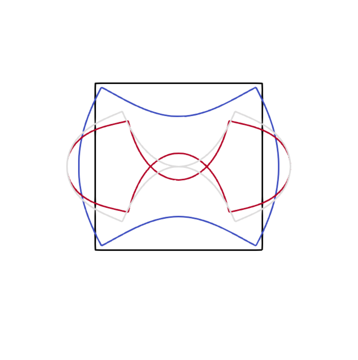
Consider first the square frame shown in Fig. 9. Its response under compressive loading is characterized by the load-displacement diagrams in Fig. 10a, with the red curve corresponding to the vertical deflection $w_{3}$ and the blue curve to the horizontal displacement $u_{1}$ (both normalized by $L$ ). Empty circles represent Mattiasson’s data and the crosses indicate three states for which the deformed shapes are plotted in Fig. 11a. Analogous results for the case of tensile loading are presented in Fig. 10b in terms of the load-displacement diagrams and in Fig. 11b in terms of the deformed shapes at three selected states.

(a)	(b)

Figure 10: Square frame: load-displacement curves for (a) compression loading, (b) tension loading. With reference to Fig. 9b, horizontal displacement

u

is reported at node 1 while vertical displacement

w

is reported at node 3. Dotted lines represent Mattiason’s solution. Crosses indicate three states for which the deformed shapes are plotted in Fig. 11.

The agreement of our results with Mattiasson’s solution is seen to be excellent. For compression, the response after reaching the load level $PL^{2}/EI$ =3.3942 (second cross in Fig. 10a) loses its physical meaning because of non-physical penetration of node 3 into its mirrored counterpart (see the deformed shape red colored in Fig. 11a). The present numerical results have been computed using 30 integration segments per element and with the axial stiffness parameter $EAL^{2}/EI$ set to $10^{6}$ . This value is fully sufficient to get very close to the inextensible limit. If the parameter is increased to $10^{7}$ , the relative change of the vertical displacement at the end of the simulation (i.e., at load level $PL^{2}/EI=4$ ) is only $3\cdot 10^{-6}$ . Even for $EAL^{2}/EI=10^{4}$ , the relative change with respect to the inextensible case would be $3\cdot 10^{-4}$ , which is still negligible. On the other hand, $EAL^{2}/EI=10^{2}$ would lead to a relative change of 2.9 % in the vertical displacement and 1.3 % in the horizontal displacement, which may already play some role. Still lower values of the axial stiffness parameter are not relevant because they correspond to deep beams for which the beam theory with neglected shear distortion would be inappropriate.

The choice of the axial stiffness parameter reflects the geometry of the frame (shape of the cross section and span-to-depth ratio). Let us now explore the effect of a numerical parameter—the number of integration segments per element. The “high-precision” value (i.e., the value computed with an extremely high number of integration segments) of normalized displacement $w_{3}/L$ computed at load level $PL^{2}/EI=4$ is 1.177368 for $EAL^{2}/EI=$ 10,000 and 1.211001 for $EAL^{2}/EI=100$ . The values obtained for various numbers of integration segments per element and the corresponding relative errors are summarized in Table 2. Already for 8 segments, the discretization error is below 1 %, and it decreases proportionally to the square of the segment size.

Table 2: Square frame: evaluation of errors in displacement caused by numerical integration along the beam elements.

	$EAL^{2}/EI=$ 10,000		$EAL^{2}/EI=$ 100
number of segments	displacement	error $[\%]$	displacement	error $[\%]$
8	1.221452	0.863	1.187822	0.888
10	1.217680	0.551	1.184051	0.568
20	1.212668	0.138	1.179036	0.142
40	1.211418	0.0344	1.177785	0.0354
80	1.211105	0.0086	1.177472	0.0089
160	1.211027	0.0022	1.177394	0.0022
320	1.211008	0.0006	1.177374	0.0005
$\to\infty$	1.211001	0	1.177368	0

Refer to caption — Figure 11: Square frame: deformed shapes (scale factor equal to 1) for (a) compression loading (b) tensile loading. The corresponding points in the load-displacement diagrams are indicated in Fig. 10 by ’+’ symbols.

The example of the square frame loaded in compression can further be exploited for illustration of convergence properties of the proposed numerical method. The objective is to explore how the computational procedure converges if a very large load increment is applied. The model deals with five global unknowns ( $u_{1}$ , $u_{2}$ , $w_{2}$ , $\varphi_{2}$ , and $w_{3}$ ), which are found iteratively by Newton-Raphson equilibrium iterations. In each iteration, the end forces and the tangent stiffness need to be evaluated for given values of the global unknowns, and this evaluation is also performed iteratively, using the technique described in Section 3.1. Each iterative process uses a certain error tolerance, which can influence the number of iterations needed to satisfy the underlying equations with sufficient accuracy.

It turns out that the numerical scheme is more robust for lower values of the axial stiffness parameter. For $EAL^{2}/EI=100$ (considered as low), it is possible to apply the total load $PL^{2}/EI=4$ in one single step, starting from the undeformed configuration. The error (defined as the norm of the unbalanced forces normalized by the same factor $EI/L^{2}$ as the actual load) first increases from 4.0 to 43.9, but after 6 iterations it is below $10^{-3}$ and after 8 iterations below $10^{-9}$ . For $EAL^{2}/EI=1000$ , the maximum step size is $\Delta PL^{2}/EI=1.99$ , and for $EAL^{2}/EI=$ 10,000, it is $\Delta PL^{2}/EI=0.6$ , which means that the whole diagram depicted in Fig. 10a can be covered respectively in 3 or 7 incremental steps. Of course, larger steps require more global Newton-Raphson iterations.

For comparison, Table 3 shows the average numbers of global iterations per step needed to increase the load to $PL^{2}/EI=4$ , depending on the step size, axial stiffness parameter and relative tolerance (maximum allowed norm of unbalanced forces normalized by $EI/L^{2}$ ). In each row, the step size is indicated in the first column and the other columns contain the average numbers of iterations per step for various combinations of parameters $(EAL^{2}/EI,\varepsilon_{\rm tol})$ , in each case specified in the column heading. For sufficiently short steps, convergence is very regular. For instance, for $EAL^{2}/EI=100$ and step size $\Delta PL^{2}/EI=0.25$ , the whole curve is covered in 16 steps and, in each step, 2 iterations are sufficient to bring the error below $10^{-3}$ and 2 additional iterations bring the error below $10^{-9}$ . On the other hand, for larger steps or higher axial stiffness, more iterations are needed in the initial part of the iterative process, during which the evolution of error is typically less regular. Once the computed approximation gets close to the exact solution, quadratic convergence is observed and the error is easily reduced from $10^{-3}$ to $10^{-9}$ in at most two iterations.

Table 3: Square frame loaded by compression: average numbers of global iterations per step, depending on

(EAL^{2}/EI,\varepsilon_{\rm tol})

where

EAL^{2}/EI=100

or 10,000 is the axial stiffness parameter and

\varepsilon_{\rm tol}=10^{-3}

10^{-9}

is the tolerance.

$\mathbf{\Delta PL^{2}/EI}$	$\mathbf{(100}$ , $\mathbf{10^{-3})}$	$\mathbf{(100}$ , $\mathbf{10^{-9})}$	$\mathbf{(10000}$ , $\mathbf{10^{-3})}$	$\mathbf{(1000}$ , $\mathbf{10^{-9})}$
4	6	8
2	4	5.5
1	4	5
0.5	3	4	5.125	6.75
0.25	2	4	4	5.438

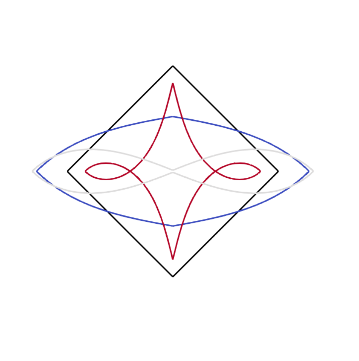
Let us now proceed to the diamond frame shown in Fig. 12. The corresponding load-displacement diagrams are plotted in Fig. 13 and the deformed shapes are shown in Fig. 14. Red color in Fig. 12 corresponds to the deflection $w_{2}$ and blue color to the horizontal displacement $u_{1}$ . The agreement of the present numerical results with Mattiason’s solution is again excellent.

(a)	(b)

Figure 12: Diamond frame: (a) Geometry and applied loads (case of compression), (b) one-quarter model that exploits symmetry, leading to three global unknowns.

(a)	(b)

Figure 13: Diamond frame: load-displacement curves for (a) compression loading, (b) tension loading. With reference to Fig. 12b, horizontal displacement

u

is reported at node 1 while vertical displacement

w

is reported at node 2. Dotted lines represent Mattiason’s solution. Crosses indicate three states for which the deformed shapes are plotted in Fig. 14.

4.5 Honeycomb lattice

4.5.1 Problem description

In the last example we consider a material with internal microstructure that corresponds to a two-dimensional elastic honeycomb lattice. Samples of such material will be subjected to prescribed displacements that would induce uniaxial tension or compression if the material behaved as a homogeneous continuum. The objective is to study the size effect, i.e., to investigate how the macroscopic response of a finite sample deviates from the limit behavior of an infinite lattice, which can be under certain conditions described using a hexagonal unit cell with imposed periodicity conditions.

The unit cell is a regular hexagon consisting of six beam elements of length $a$ , as shown in Fig. 15a. Larger assemblies are obtained by stacking the cells horizontally and vertically in a honeycomb pattern. For instance, the assembly in Fig. 15b will be referred to as the $3\times 3$ pattern. It can be considered as consisting of 3 layers; the odd layers contain 3 cells each while the even layer contains 2 full cells and 2 half-cells. Similarly, the assembly in Fig. 15c represents the $11\times 11$ pattern.

(a)	(b)	(c)

Figure 15: Honeycomb lattices: (a) regular hexagonal cell with numbering of nodes and global coordinate system, (b)

3\times 3

lattice, (c)

11\times 11

lattice.

The projected dimensions of the unit cell are $B_{1}=a\sqrt{3}$ horizontally and $H_{1}=2a$ vertically. In general, an $n\times n$ lattice has width $B_{n}=na\sqrt{3}$ and height $H_{n}=(3n+1)a/2$ . The lattices are loaded by tension or compression in the vertical direction. The loading is applied by prescribed monotonically increasing vertical displacements $\bar{w}$ at $n$ bottom nodes with coordinate $z=H_{n}$ , while the $n$ top nodes with coordinate $z=0$ are constrained vertically (prescribed displacements $w=0$ ). All nodes are free to move horizontally, only one node (an arbitrary one) is fixed horizontally in order to suppress rigid body translations.

4.5.2 Hexagonal unit cell with periodic conditions

For uniaxial tension or compression of an infinite lattice in the vertical direction, the solution can be expected to exhibit periodicity and symmetry with respect to the horizontal and vertical axes of each hexagonal cell (unless it is disturbed by instabilities, which are currently disregarded). Periodicity conditions combined with symmetry lead to zero rotations of all joints. Moreover, due to symmetry, vertical beams 1-6 and 3-4 deform only axially, and the deformation of the four inclined beams can be obtained by mirroring the deformation pattern of one of them (Fig. 16a). Consequently, it is sufficient to analyze only one selected inclined beam with one end clamped and the other forced to displace vertically and allowed to move horizontally (Fig. 16b). Once the forces in this beam are computed, the axial force in vertical beams is obtained from equilibrium and the macroscopic strain and stress can be evaluated.

In the incompressible limit, the behavior of the inclined beam in Fig. 16b can be described analytically. One can even further reduce the problem to a cantilever of length $a/2$ shown in Fig. 16c, because the inflexion point must be located at midspan of the original beam of length $a$ . When the cantilever is analyzed in its local coordinate system, the problem is equivalent to the one solved in Appendix A.5 and depicted in Fig. 20, with the direction of the applied force inclined by $\alpha=2\pi/3$ with respect to the beam axis in the undeformed state (Fig. 16d). Formulae (189)–(192) derived in the appendix are directly applicable, with cantilever length $L$ set to $a/2$ .

(a)	(b)	(c)	(d)

Figure 16: Hexagonal unit cell with periodic conditions: (a) deformed cell under tension, (b) upper left inclined beam with boundary conditions that follow from periodicity and double symmetry, (c) upper half of the inclined beam, (d) rotated cantilever (the straight dashed line is the undeformed shape).

The end-point displacements $u_{a}$ and $w_{a}$ given by (190)–(191) refer to the local beam coordinates, but their projection onto the direction of the applied force, $u_{F}$ , which can be evaluated from (192), corresponds to one half of the difference between global vertical displacements of nodes 5 and 6 of the unit cell. Since the vertical displacements of nodes 6 and 1 are the same (due to inextensibility of the vertical beam that connects these nodes), the difference between global vertical displacements of nodes 5 and 1 is $2\,u_{F}$ , and the corresponding macroscopic normal strain in the periodic lattice in the vertical direction is

\varepsilon_{z}=\frac{2u_{F}}{3H_{1}/4}=\frac{4u_{F}}{3\,a}

(119)

The force $F$ evaluated from (189) can be converted into the macroscopic normal stress

\sigma_{z}=\frac{F}{tB_{1}/2}=\frac{2F}{ta\sqrt{3}}

(120)

Here, $t$ denotes the out-of-plane thickness.

Based on formulae (189) and (192) and on the transformation of displacement and force into strain and stress given by (119)–(120), it is possible to construct the stress-strain diagram. In (189) and (192), the force and the displacement are expressed as functions of the rotation of the free end, which plays the role of a parameter. In the analysis presented in Appendix A.5, $F$ is considered as a positive quantity that represents the magnitude of the force, and the oriented direction is taken into account by an appropriate choice of angle $\alpha$ . For tension, $\alpha$ needs to be set to $2\,\pi/3$ . Since the analytical solution derived in Appendix A.5 is valid for $\alpha$ between 0 and $\pi$ , vertical compression of the honeycomb lattice needs to be handled by setting $\alpha=\pi/3$ and adding negative signs in front of the fractions in (119)–(120).

The macroscopic stress-strain curves extracted from the results obtained for one hexagonal cell with imposed periodicity are plotted in both parts of Fig. 17. The dashed black curve represents the analytical solution derived for axially inextensible beams and the red curve has been obtained by a numerical simulation of the inclined beam 5-6 considered as extensible, with the contribution of the vertical (also extensible) beam 6-1 added in closed form. The dimensionless stress plotted in Fig. 17 is the actual macroscopic stress divided by the normalizing factor $EI/(ta^{3})$ . The simulations have been performed with a relatively high normal stiffness characterized by the dimensionless parameter $EAa^{2}/EI=10,000$ . The numerical and analytical results are in very good agreement and the red and dashed black curves slightly differ only in the regime of high tension, as seen more clearly in Fig. 18.

(a)	(b)

Figure 17: Honeycomb lattice, complete stress-strain curves: (a) raw results, (b) results with compensation for missing stiff layer.

(a)	(b)

Figure 18: Honeycomb lattice, stress-strain curves for tension: (a) raw results, (b) results with compensation for missing stiff layer.

4.5.3 Effect of lattice size

The solutions that satisfy periodicity conditions correspond to the theoretical limit of an infinite lattice filling the whole plane. To assess the effect of finite size, numerical simulations have been performed on finite $n\times n$ lattices exemplified in Fig. 15b,c, with $n=1,3,5$ and 11. The imposed vertical displacement $\bar{w}$ and the computed reactions at the bottom nodes, $R_{i}$ , $i=1,2,\ldots n$ , have been converted into the corresponding average stress and strain,

	$\displaystyle\sigma$	$\displaystyle=$	$\displaystyle\frac{\sum_{i=1}^{n}R_{i}}{tB_{n}}$		(121)
	$\displaystyle\varepsilon$	$\displaystyle=$	$\displaystyle\frac{\bar{w}}{H_{n}}$		(122)

Stress-strain curves obtained in this way are shown in Figs. 17a and 18a. A strong size effect is observed—smaller samples lead to a more compliant response, both in tension and in compression. The overall shapes of all stress-strain curves are similar. Only a slight nonlinearity is observed in compression while the tensile response is highly nonlinear, with a dramatic increase of tangent stiffness at average strains exceeding 10 %. This stiffening is caused by the fact that the inclined beams initially deform by bending but this relatively soft deformation mode has a limited capacity and as the inclined beams get aligned with the direction of applied tensile loading, their high axial stiffness is activated. This is nicely illustrated by the deformed shapes in parts (a) and (c) of Fig. 19.

The size effect exhibited by the stress-strain diagrams in Fig. 17a is to some extent caused by the fact that the finite lattices of the kind depicted in Fig. 15b,c do not represent a decomposition of the infinite lattice into periodically repeatable units. Indeed, when we stack two such lattices vertically, an additional layer of vertical beams needs to be inserted in between, and when we stack them horizontally, the vertical beams on the boundaries that are now glued together would be doubled.

The first effect turns out to be stronger than the second one. It can be eliminated by adding an extra layer of vertical beams to the nodes at the bottom of each lattice. The resulting modified lattice would not be practical for testing but its numerical treatment is straightforward. In fact, it is not even necessary to perform additional numerical simulations of the modified lattices because the effect of the added layer on the stress-strain diagram can easily be estimated. At a given stress $\sigma$ evaluated from (121), the average axial force in the vertical beams is equal to the average reaction, $\bar{R}=\sigma tB_{n}/n$ , and the contribution of the added layer of axially deformed beams to the vertical displacement on the boundary is $\Delta\bar{w}=\bar{R}a/EA$ . At the same time, the added layer increases the height of the sample by $\Delta H=a$ . The corrected average strain is then estimated as

\varepsilon+\Delta\varepsilon=\frac{\bar{w}+\Delta\bar{w}}{H_{n}+\Delta H}=\frac{\varepsilon(3n+1)a/2+\bar{R}a/EA}{(3n+1)a/2+a}=\frac{\varepsilon(3n+1)+2\sigma ta\sqrt{3}/EA}{3n+3}=\frac{3n+1}{3(n+1)}\,\varepsilon+\frac{2ta}{\sqrt{3}\,(n+1)EA}\,\sigma

(123)

from which

\Delta\varepsilon=-\frac{2}{3(n+1)}\,\varepsilon+\frac{2}{\sqrt{3}\,(n+1)}\,\frac{EI}{EAa^{2}}\,\frac{\sigma ta^{3}}{EI}

(124)

For beams with high axial stiffness, the second term on the right-hand side is usually negligible compared to the first term. It is expressed as a product of three fractions, the second of which is the reciprocal value of the dimensionless stiffness coefficient $EAa^{2}/EI$ , in our example equal to 10,000. In Fig. 17, normalized stresses $\sigma ta^{3}/EI$ do not exceed 30, and so even for $n=1$ the strain correction described by the second term on the right-hand side of (124) is $30/(10,000\cdot\sqrt{3})\approx 0.0017$ . On the other hand, the first term on the right-hand side of (124) is important, especially for small $n$ . The strain correction $\Delta\varepsilon$ has the opposite sign than the originally evaluated strain $\varepsilon$ , which means that the correction leads to stiffer response.

Stress-strain diagrams for the modified lattices with an added layer of vertical beams are shown in . The size effect is reduced, but it is still present, especially for small lattices. The residual size effect originates from softer response of cells located near the lateral (vertical) boundaries of the sample. For a large lattice, cells that are far from the lateral boundaries deform in a pattern similar to the periodic cell, i.e., with negligible rotations. On the other hand, cells located in boundary layers are less constrained and deform more easily. Images of deformed lattices in Fig. 19 indicate that nodes on the lateral boundaries rotate and the deformation is more equally distributed among the vertical and inclined beams, which reduces the apparent macroscopic stiffness of the sample. Since the affected boundary layers occupy a relatively larger area fraction in a small sample than in a large one, smaller samples behave as if the material were softer.

5 Concluding remarks

The geometrically nonlinear formulation of a beam element developed in this paper is based on kinematic equations valid for arbitrarily large rotations of cross sections. These equations are combined with the integrated form of equilibrium equations and with generalized material equations that link the internal forces to the deformation variables (curvature and centerline stretch). The resulting fundamental equations have the form of a set of three first-order ordinary differential equations for two displacements and one rotation as basic unknowns. Instead of approximating these functions by apriori selected shape functions, it is proposed to convert the boundary value problem into an initial value problem using a technique inspired by the shooting method, and then to adopt a finite difference scheme. The advantage is that accuracy of the numerical approximation can be conveniently increased by refining the integration scheme on the element level while the number of global degrees of freedom is kept constant.

A number of examples have been presented to illustrate the flexibility and efficiency of the proposed approach and to assess its accuracy and robustness. In all examples, the number of global degrees of freedom has been kept as low as possible. Spatial refinement has been taken care of by reducing the spacing between auxiliary grid points used for finite-difference approximation of the fundamental equations. The results have been shown to be in excellent agreement with previously published numerical results or analytical solutions. For the Williams toggle frames, a good agreement with experimental data has been observed.

It has been shown that when the integration grid is refined, the error decreases in proportion to the square of the grid spacing. The accuracy is comparable to results obtained when the beam is discretized by standard finite elements of the same size as the grid spacing. However, the present approach has the big advantage that no additional global degrees of freedom need to be introduced when the grid is refined. In the context of an incremental iterative analysis on the global (structural) level, relatively large increments of nodal displacements and rotations can be handled. The shooting method adopted on the element level at the same time permits to set up the element tangent stiffness matrix, which is then processed by a standard assembly procedure to construct the structural tangent stiffness. Linearization of the global equations is consistent, as confirmed by quadratic convergence of the global Newton-Raphson iteration procedure. This process is more robust for low values of the axial stiffness (reflected by the dimensionless stiffness parameter $EAL^{2}/EI$ ), and for higher values it works fine provided that the increment size is not extreme.

To keep the paper focused and its size limited, we have presented a basic version of the proposed approach, with a number of simplifying assumptions. For instance, the stress-strain law has been assumed to be linear elastic, and the beam element has been considered as two-dimensional and initially straight. This relatively simple setting permits to explain the main ideas and highlight the essence of the numerical procedure. However, extensions and generalizations are possible and some of them are currently being explored. In particular, an extension to beam elements with initial curvature seems to be potentially attractive and powerful, and it will be reported on in a follow-up publication.

Acknowledgments

The authors acknowledge the support of the Czech Science Foundation (project No. 19-26143X).

Conflict of interest

The authors declare no potential conflict of interests.

Appendix A Nonlinear elastic beam – analytical treatment

A.1 Solution of second-order equation for sectional rotation

The problem described by equations (37)–(39), which were derived in Section 2.3.1 and form the basis of the algorithms used in this paper, can be handled analytically. It is convenient to start from the transformed version of these equations given in (40), because it contains the rotation function $\varphi$ as the only unknown. Equation (40) is a nonlinear second-order differential equation in a special form

\varphi^{\prime\prime}+g(\varphi)=0

(125)

and it always allows for a formal “analytical” solution. The usefulness of the result depends on the existence of closed-form expressions for integrals that are arise in the solution process.

To derive a formal analytical solution, let us first multiply (125) by $2\varphi^{\prime}$ and then express the resulting equation as

\left(\varphi^{\prime 2}+2G(\varphi)\right)^{\prime}=0

(126)

where $G$ is the indefinite integral (antiderivative) of $g$ . The resulting first-order equation

\varphi^{\prime 2}+2G(\varphi)=C

(127)

can be handled by separation of variables, which leads to

\pm\frac{{\textrm{d}}\varphi}{\sqrt{C-2G(\varphi)}}={\textrm{d}}x

(128)

and finally to the implicit formula for the solution,

\pm\int_{\varphi_{0}}^{\varphi(x)}\frac{{\textrm{d}}\bar{\varphi}}{\sqrt{C-2G(\bar{\varphi})}}=x-x_{0}

(129)

Here, $C$ is an arbitrary integration constant, and $\varphi_{0}$ is the value of $\varphi$ at $x=x_{0}$ . The sign to be used in front of the integral corresponds to the sign of the first derivative of $\varphi$ in the interval of interest.

When this technique is applied to equation (40), the corresponding function $g$ is given by

	$\displaystyle g(\varphi)$	$\displaystyle=$	$\displaystyle\frac{1}{EI}\left(1+\frac{-X_{ab}\cos\varphi+Z_{ab}\sin\varphi}{EA}\right)\left(X_{ab}\sin\varphi+Z_{ab}\cos\varphi\right)=$		(130)
		$\displaystyle=$	$\displaystyle\frac{X_{ab}}{EI}\sin\varphi+\frac{Z_{ab}}{EI}\cos\varphi+\frac{Z_{ab}^{2}-X_{ab}^{2}}{2EIEA}\sin 2\varphi-\frac{Z_{ab}X_{ab}}{EIEA}\cos 2\varphi$		(130)

Integration with respect to $\varphi$ is easy and the antiderivative of $g$ can be selected as

G(\varphi)=\frac{X_{ab}}{EI}\left(1-\cos\varphi\right)+\frac{Z_{ab}}{EI}\sin\varphi+\frac{Z_{ab}^{2}-X_{ab}^{2}}{4EIEA}\left(1-\cos 2\varphi\right)-\frac{Z_{ab}X_{ab}}{2EIEA}\sin 2\varphi

(131)

For initial conditions

	$\displaystyle\varphi(0)$	$\displaystyle=$	$\displaystyle\varphi_{a}$		(132)
	$\displaystyle\varphi^{\prime}(0)$	$\displaystyle=$	$\displaystyle\kappa_{a}$		(133)

we obtain integration constant

C=\kappa_{a}^{2}+2G(\varphi_{a})

(134)

expressed in terms of the left-end rotation, $\varphi_{a}$ , and left-end curvature, $\kappa_{a}$ .

Up to here, everything has been quite straightforward. However, in the next step we need to evaluate the integral on the left-hand side of (129), which is given by

\int\frac{{\rm d}\bar{\varphi}}{\sqrt{\kappa_{a}^{2}+2G(\varphi_{a})-2G(\bar{\varphi})}}=\int\frac{{\rm d}\bar{\varphi}}{\sqrt{c_{1}+c_{2}\cos\bar{\varphi}+c_{3}\sin\bar{\varphi}+c_{4}\cos 2\bar{\varphi}+c_{5}\sin 2\bar{\varphi}}}

(135)

In general, this would be very difficult. In the special case of an axially inextensible beam, the problem is simplified because coefficients $c_{4}$ and $c_{5}$ , which multiply the terms with $\cos 2\bar{\varphi}$ and $\sin 2\bar{\varphi}$ , vanish (they contain $EA$ in the denominator). The remaining coefficients are given by

$\displaystyle c_{1}$	$\displaystyle=$	$\displaystyle\kappa_{a}^{2}-\frac{2X_{ab}}{EI}\cos\varphi_{a}+\frac{2Z_{ab}}{EI}\sin\varphi_{a}=\kappa_{a}^{2}+\frac{2N_{ab}}{EI}$	(136)
$\displaystyle c_{2}$	$\displaystyle=$	$\displaystyle\frac{2X_{ab}}{EI}$	(137)
$\displaystyle c_{3}$	$\displaystyle=$	$\displaystyle-\frac{2Z_{ab}}{EI}$	(138)

in which

N_{ab}=-X_{ab}\cos\varphi_{a}+Z_{ab}\sin\varphi_{a}

(139)

is the normal force at the left end section. Let us introduce auxiliary constants,

$\displaystyle F_{ab}$	$\displaystyle=$	$\displaystyle\sqrt{X_{ab}^{2}+Z_{ab}^{2}}$	(140)
$\displaystyle A$	$\displaystyle=$	$\displaystyle\sqrt{c_{2}^{2}+c_{3}^{2}}=\frac{2}{EI}\sqrt{X_{ab}^{2}+Z_{ab}^{2}}=\frac{2F_{ab}}{EI}$	(141)
$\displaystyle\alpha$	$\displaystyle=$	$\displaystyle-\arctan\frac{c_{3}}{c_{2}}=\arctan\frac{Z_{ab}}{X_{ab}}$	(142)

and a transformed variable,

\tilde{\varphi}=\frac{\bar{\varphi}+\alpha}{2}

(143)

Their purpose is to replace $c_{2}\cos\bar{\varphi}+c_{3}\sin\bar{\varphi}$ by $A\cos 2\tilde{\varphi}=A(1-2\sin^{2}\tilde{\varphi})$ . Then we can proceed to the integral

	$\displaystyle\int_{\varphi_{a}}^{\varphi}\frac{{\rm d}\bar{\varphi}}{\sqrt{c_{1}+c_{2}\cos\bar{\varphi}+c_{3}\sin\bar{\varphi}}}$	$\displaystyle=$	$\displaystyle\int_{(\varphi_{a}+\alpha)/2}^{(\varphi+\alpha)/2}\frac{2\,{\rm d}\tilde{\varphi}}{\sqrt{c_{1}+A(1-2\sin^{2}\tilde{\varphi})}}=\frac{2}{\sqrt{c_{1}+A}}\int_{(\varphi_{a}+\alpha)/2}^{(\varphi+\alpha)/2}\frac{{\rm d}\tilde{\varphi}}{\sqrt{1-\displaystyle\frac{2A}{c_{1}+A}\sin^{2}\tilde{\varphi}}}=$		(144)
		$\displaystyle=$	$\displaystyle\frac{2}{\sqrt{c_{1}+A}}\int_{(\varphi_{a}+\alpha)/2}^{(\varphi+\alpha)/2}\frac{{\rm d}\tilde{\varphi}}{\sqrt{1-k^{2}\sin^{2}\tilde{\varphi}}}$		(144)

where

k=\sqrt{\frac{2A}{c_{1}+A}}=\sqrt{\frac{4F_{ab}}{2(F_{ab}+N_{ab})+EI\kappa_{a}^{2}}}

(145)

Recall that $F_{ab}$ given by (140) is the magnitude of the end force, which is by definition non-negative. It is worth noting that the denominator of the fraction under the square root in (145), given by $2(F_{ab}+N_{ab})+EI\kappa_{a}^{2}$ , is also non-negative because $N_{ab}\geq-F_{ab}$ . This denominator could be zero only if $N_{ab}=-F_{ab}$ and $\kappa_{a}=0$ (equivalent to $M_{ab}=0$ ), which is the case of uniaxial tension, leading to the trivial solution $\varphi(x)=0$ .

Now we can substitute the right-hand side of (144) into (129), setting $x_{0}=0$ and $\varphi_{0}=\varphi_{a}$ and selecting the sign in front of the integral as ${\rm sgn}\,\kappa_{a}$ , so that it agrees with the sign of $\varphi^{\prime}$ at $x=0$ . If the curvature at the left end, $\kappa_{a}$ , happens to be zero (in cases when the end moment $M_{ab}$ vanishes), the sign should correspond to the expected sign of the curvature for small positive values of $x$ , which can be deduced from $\alpha$ and $\varphi_{a}$ .

The integral on the left-hand side of (129) is evaluated for function

G(\varphi)=\frac{X_{ab}}{EI}\left(1-\cos\varphi\right)+\frac{Z_{ab}}{EI}\sin\varphi

(146)

which is the reduced version of (131) valid for an axially inextensible beam ( $EA\to\infty$ ). Constant $C$ is substituted from (134) and the integral is expressed based on (144). The resulting equation

\frac{2\,{\rm sgn}\,\kappa_{a}}{\sqrt{c_{1}+A}}\int_{(\varphi_{a}+\alpha)/2}^{(\varphi(x)+\alpha)/2}\frac{{\rm d}\tilde{\varphi}}{\sqrt{1-k^{2}\sin^{2}\tilde{\varphi}}}=x

(147)

implicitly defines function $\varphi(x)$ that describes the sectional rotation.

A.2 Mathematical tools – elliptic integrals and elliptic functions

The integral on the right-hand side of (147) is recognized as one of the elliptic integrals. Before we proceed with the solution, let us recall the definitions of elliptic integrals and elliptic functions, which will later be used in analytical expressions describing the rotation and displacement functions. A systematic overview can be found in standard mathematical literature, e.g., in [17].

The incomplete elliptic integral of the first kind is given by

{\rm F_{J}}(\varphi,k)=\int_{0}^{\varphi}\frac{{\rm d}t}{\sqrt{1-k^{2}\sin^{2}t}}

(148)

If the upper bound in the integral is set to $\pi/2$ , we obtain the complete elliptic integral of the first kind,

{\rm K}(k)={\rm F_{J}}(\pi/2,k)=\int_{0}^{\pi/2}\frac{{\rm d}t}{\sqrt{1-k^{2}\sin^{2}t}}

(149)

The Jacobi amplitude function ${\rm am}(x,k)$ is the inverse of ${\rm F_{J}}$ with respect to $\varphi$ , with $k$ considered as a fixed parameter (again, usually in the range between 0 and 1). This means that

{\rm am}(x,k)=\varphi

(150)

is equivalent with

x={\rm F_{J}}(\varphi,k)

(151)

The elliptic sine and elliptic cosine are defined as

	$\displaystyle{\rm sn}(x,k)$	$\displaystyle=$	$\displaystyle\sin({\rm am}(x,k))$		(152)
	$\displaystyle{\rm cn}(x,k)$	$\displaystyle=$	$\displaystyle\cos({\rm am}(x,k))$		(153)

and belong to the family of Jacobi elliptic functions. Another useful member of this family is the so-called delta amplitude

{\rm dn}(x,k)=\sqrt{1-k^{2}\,{\rm sn}^{2}(x,k)}

(154)

Finally, the incomplete and complete elliptic integrals of the second kind are defined as

	$\displaystyle{\rm E_{J}}(\varphi,k)$	$\displaystyle=$	$\displaystyle\int_{0}^{\varphi}\sqrt{1-k^{2}\sin^{2}t}\,{\rm d}t$		(155)
	$\displaystyle{\rm E}(k)$	$\displaystyle=$	$\displaystyle{\rm E_{J}}(\pi/2,k)=\int_{0}^{\pi/2}\sqrt{1-k^{2}\sin^{2}t}\,{\rm d}t$		(156)

In the above expressions, parameter $k$ is usually considered in the range between 0 and 1. The integrals in (148) and (155) are well defined even for $k>1$ as long as $\varphi$ remains below $\arcsin(1/k)$ . However, some implementations of incomplete elliptic integrals and elliptic functions consider the case of $k>1$ as inadmissible, for any $\varphi$ . One can then exploit the transformation

{\rm F_{J}}(\varphi,k)=\int_{0}^{\varphi}\frac{{\rm d}t}{\sqrt{1-k^{2}\sin^{2}t}}=\frac{1}{k}\int_{0}^{\arcsin(k\sin\varphi)}\frac{{\rm d}s}{\sqrt{1-k^{-2}\sin^{2}s}}=\frac{1}{k}{\rm F_{J}}(\arcsin(k\sin\varphi),1/k)

(157)

and use function ${\rm F_{J}}$ with parameter $k>1$ replaced by its reciprocal value, $\tilde{k}=1/k<1$ . Based on (157), we can also write

{\rm am}(x,k)=\arcsin\frac{\sin{\rm am}(kx,1/k)}{k}

(158)

In terms of the elliptic sine function, formula (158) can be rewritten in an elegant form

{\rm sn}(x,k)=\frac{1}{k}\,{\rm sn}\left(kx,\frac{1}{k}\right)

(159)

Analogous expressions can be derived for the other elliptic functions and for the incomplete elliptic integral of the second kind. In summary, the expressions useful for conversion of $k$ into its reciprocal value read

$\displaystyle{\rm am}(x,k)$	$\displaystyle=$	$\displaystyle\arcsin(\tilde{k}\,{\rm sn}(x/\tilde{k},\tilde{k}))$	(160)
$\displaystyle{\rm sn}(x,k)$	$\displaystyle=$	$\displaystyle\tilde{k}\,{\rm sn}(x/\tilde{k},\tilde{k})$	(161)
$\displaystyle{\rm cn}(x,k)$	$\displaystyle=$	$\displaystyle{\rm dn}(x/\tilde{k},\tilde{k})$	(162)
$\displaystyle{\rm dn}(x,k)$	$\displaystyle=$	$\displaystyle{\rm cn}(x/\tilde{k},\tilde{k})$	(163)
$\displaystyle{\rm F_{J}}(\varphi,k)$	$\displaystyle=$	$\displaystyle\tilde{k}\,{\rm F_{J}}(\tilde{\varphi},\tilde{k})$	(164)
$\displaystyle{\rm E_{J}}(\varphi,k)$	$\displaystyle=$	$\displaystyle{\rm E_{J}}(\tilde{\varphi},\tilde{k})/\tilde{k}+(\tilde{k}-1/\tilde{k})\,{\rm F_{J}}(\tilde{\varphi},\tilde{k})$	(165)

in which $k=1/\tilde{k}$ and $k\sin\varphi=\sin\tilde{\varphi}$ .

A.3 Expressions for rotation and displacement functions

Let us get back to the beam deformation problem. Making use of the definition of the incomplete elliptic integral of the first kind, ${\rm F_{J}}$ , equation (147) can be written as

\frac{2\,{\rm sgn}\,\kappa_{a}}{\sqrt{c_{1}+A}}\left({\rm F_{J}}\left(\frac{\varphi(x)+\alpha}{2},k\right)-{\rm F_{J}}\left(\frac{\varphi_{a}+\alpha}{2},k\right)\right)=x

(166)

from which

\varphi(x)=2\,{\rm am}\left(a+bx,k\right)-\alpha

(167)

where

	$\displaystyle a$	$\displaystyle=$	$\displaystyle{\rm F_{J}}\left(\frac{\varphi_{a}+\alpha}{2},k\right)$		(168)
	$\displaystyle b$	$\displaystyle=$	$\displaystyle\frac{\sqrt{c_{1}+A}}{2}\,{\rm sgn}\,\kappa_{a}$		(169)

This is the analytical solution for the sectional rotation $\varphi$ as function of the local coordinate $x$ . Auxiliary constants $\alpha$ , $k$ , $c_{1}$ and $A$ depend on the end forces and moment at the left end of the beam and on the rotation of the left end section (note that $\kappa_{a}=-M_{ab}/EI$ ). Of course, not all of these variables are prescribed in advance and they need to be determined from appropriate boundary conditions.

Based on expression (167) for the sectional rotation, it is possible to evaluate

	$\displaystyle\sin\varphi(x)$	$\displaystyle=$	$\displaystyle 2\cos\alpha\,{\rm sn}(a+bx,k)\,{\rm cn}(a+bx,k)-\sin\alpha\,(1-2\,{\rm sn}^{2}(a+bx,k))$		(170)
	$\displaystyle\cos\varphi(x)$	$\displaystyle=$	$\displaystyle 2\sin\alpha\,{\rm sn}(a+bx,k)\,{\rm cn}(a+bx,k)+\cos\alpha\,(1-2\,{\rm sn}^{2}(a+bx,k))$		(171)

When this is substituted into the right-hand sides of (35)–(36) with $\lambda_{s}$ set to 1 (in accordance with the assumption of axial inextensibility), integration of the resulting equations leads to analytical expressions for displacement functions,

	$\displaystyle u_{s}(x)$	$\displaystyle=$	$\displaystyle C_{u}-x-\frac{2}{bk^{2}}\,{\rm dn}(a+bx,k)\sin\alpha+\left(\frac{2}{bk^{2}}{\rm E_{J}}({\rm am}(a+bx,k),k)+x-\frac{2x}{k^{2}}\right)\cos\alpha$		(172)
	$\displaystyle w_{s}(x)$	$\displaystyle=$	$\displaystyle C_{w}+\frac{2}{bk^{2}}\,{\rm dn}(a+bx,k)\cos\alpha+\left(\frac{2}{bk^{2}}{\rm E_{J}}({\rm am}(a+bx,k),k)+x-\frac{2x}{k^{2}}\right)\sin\alpha$		(173)

in which $C_{u}$ and $C_{w}$ are integration constants that need to be determined from the boundary conditions.

In cases when $k>1$ , the derived formulae for the sectional rotation and centerline displacements can be transformed into expressions that use parameter $\tilde{k}=1/k$ . It is worth noting that the case of $k>1$ arises if $A>c_{1}$ , which is equivalent to $2F_{ab}(1+\cos(\varphi_{a}+\alpha))>M_{ab}^{2}/EI$ . Making use of identities (160), (163) and (165), we obtain

$\displaystyle\varphi(x)$	$\displaystyle=$	$\displaystyle 2\,\arcsin(\tilde{k}\,{\rm sn}(\tilde{a}+\tilde{b}x,\tilde{k}))-\alpha$	(174)
$\displaystyle u_{s}(x)$	$\displaystyle=$	$\displaystyle C_{u}-x-\frac{2\tilde{k}}{\tilde{b}}\,{\rm cn}(\tilde{a}+\tilde{b}x,\tilde{k})\sin\alpha+\left(\frac{2}{\tilde{b}}\,{\rm E_{J}}({\rm am}(\tilde{a}+\tilde{b}x,\tilde{k}),\tilde{k})-x\right)\cos\alpha$	(175)
$\displaystyle w_{s}(x)$	$\displaystyle=$	$\displaystyle C_{w}+\frac{2\tilde{k}}{\tilde{b}}\,{\rm cn}(\tilde{a}+\tilde{b}x,\tilde{k})\cos\alpha+\left(\frac{2}{\tilde{b}}\,{\rm E_{J}}({\rm am}(\tilde{a}+\tilde{b}x,\tilde{k}),\tilde{k})-x\right)\sin\alpha$	(176)

where

$\displaystyle\tilde{k}$	$\displaystyle=$	$\displaystyle\frac{1}{k}=\sqrt{\frac{c_{1}+A}{2A}}=\sqrt{\frac{2(F_{ab}+N_{ab})+EI\kappa_{a}^{2}}{4F_{ab}}}=\sqrt{\sin^{2}\frac{\varphi_{a}+\alpha}{2}+\frac{M_{ab}^{2}}{4EIF_{ab}}}$	(177)
$\displaystyle\tilde{a}$	$\displaystyle=$	$\displaystyle ka=\sqrt{\frac{2A}{c_{1}+A}}{\rm F_{J}}\left(\frac{\varphi_{a}+\alpha}{2},k\right)={\rm F_{J}}\left(\arcsin\left(\frac{1}{\tilde{k}}\sin\frac{\varphi_{a}+\alpha}{2}\right),\tilde{k}\right)$	(178)
$\displaystyle\tilde{b}$	$\displaystyle=$	$\displaystyle kb=\sqrt{\frac{2A}{c_{1}+A}}\frac{{\rm sgn}\,\kappa_{a}}{2}\sqrt{c_{1}+A}=\sqrt{\frac{A}{2}}\,{\rm sgn}\,\kappa_{a}=\sqrt{\frac{F_{ab}}{EI}}\,{\rm sgn}\,\kappa_{a}$	(179)

It is worth noting that the solution described by (167) or (174) is valid only as long as the sign of the curvature does not change. If the sign changes inside the interval of interest $(0,L)$ that represents the analyzed beam of length $L$ , formula (167) can be used only up to the inflexion point of the deformed centerline. A systematic treatment of deformed shapes with inflexion points is presented in Appendix A.6 and leads to formula (207).

A.4 Special cases – straight beam and uniformly curved beam

The special case with zero denominator in (145) needs to be treated separately. This happens only if $M_{ab}=0$ and $N_{ab}=-F_{ab}$ , the latter condition leading to $\sin(\varphi_{a}+\alpha)=0$ . Inspection of the original equation (40) with initial conditions $\varphi(0)=-\alpha$ and $\varphi^{\prime}(0)=0$ shows that, in this particular case, the solution is $\varphi(x)=-\alpha$ , i.e., it is constant. The first derivative, $\varphi^{\prime}(x)$ , identically vanishes, which explains why the general solution procedure developed in Section A.1 is not applicable to this particular case (recall that the procedure started by multiplying both sides of the original equations by function $\varphi^{\prime}(x)$ ).

Another special case arises when $M_{ab}\neq 0$ and $X_{ab}=Z_{ab}=0$ , because then $c_{1}=\kappa_{a}^{2}$ , $A=0$ , $\alpha$ is undetermined and $k=0$ . For $k=0$ , functions ${\rm F_{J}}$ and “am” reduce to identities, i.e., ${\rm F_{J}}(\varphi,0)=\varphi$ and ${\rm am}(x,0)=x$ . Formulae (168)–(169) yield $a=\varphi_{a}/2$ and $b=\kappa_{a}/2$ , and the rotation function is according to (167) given by

\varphi(x)=2a+2bx=\varphi_{a}+\kappa_{a}x

(180)

This is the case of a beam with constant curvature, loaded at its end sections only by two moments of the same magnitude but opposite orientations.

A.5 Example – cantilever loaded by an inclined force

As a more challenging example, consider a cantilever fixed at its right end and loaded at its left end by a force of magnitude $F$ along an inclined line. The horizontal and vertical components of the applied force correspond to the left-end forces $X_{ab}$ and $Z_{ab}$ , and formula (142) indicates that parameter $\alpha$ used by the analytical solution is equal to the angle by which the oriented direction of the force deviates from the $x$ -axis, measured clockwise. Therefore, this angle can be directly denoted as $\alpha$ and considered as a given quantity, as shown in Fig. 20. The left-end moment, $M_{ab}$ , is set equal to zero.

(a)	(b)

Figure 20: Cantilever fixed at its right end and loaded at its left end by an inclined force: (a) Geometry in the undeformed state, (b) deformed state with

\alpha

denoting the inclination angle of the applied force (positive clockwise) and

\varphi_{a}

denoting the left-end rotation (positive anti-clockwise)

Without loss of generality, we can assume that $\alpha\in[0,\pi)$ , and it is reasonable to expect that the curvature $\kappa(x)$ has a negative sign for $x\in(0,L]$ and that $\alpha+\varphi_{a}\in[0,\pi]$ . Auxiliary constants needed to construct the analytical solution are now evaluated as follows:

$\displaystyle\tilde{k}$	$\displaystyle=$	$\displaystyle\sin\frac{\alpha+\varphi_{a}}{2}$	(181)
$\displaystyle\tilde{a}$	$\displaystyle=$	$\displaystyle{\rm F_{J}}\left(\arcsin 1,\tilde{k}\right)={\rm F_{J}}(\pi/2,\tilde{k})={\rm K}(\tilde{k})$	(182)
$\displaystyle\tilde{b}$	$\displaystyle=$	$\displaystyle-\sqrt{\frac{F}{EI}}$	(183)

Note that $\alpha$ is a given angle while the value of the left-end rotation, $\varphi_{a}$ , is related to the applied force $F$ and increases from 0 to positive values that never exceed $\pi-\alpha$ (unless $\alpha=\pi$ , in which case the beam is under axial tension and $\varphi_{a}$ remains equal to 0). Parameter $\tilde{k}$ given by (181) never exceeds 1, and so it is preferable to use elliptic functions and elliptic integrals with parameter $\tilde{k}$ and not $k$ . In the evaluation of parameter $\tilde{b}$ according to formula (179), we have replaced ${\rm sgn}\;\kappa_{a}$ , which would be zero, by the signum of the curvature in the neighborhood of the left end, which is expected to be $-1$ if $\alpha\in(0,\pi)$ . This explains the negative sign in (183).

The analytical solution for the rotation function is given in (174), and substitution into boundary condition $\varphi(L)=0$ leads to

2\,\arcsin(\tilde{k}\,{\rm sn}(\tilde{a}+\tilde{b}L,\tilde{k}))-\alpha=0

(184)

which is satisfied if

\tilde{a}+\tilde{b}L={\rm F_{J}}\left(\arcsin\left(\frac{1}{\tilde{k}}\sin\frac{\alpha}{2}\right),\tilde{k}\right)

(185)

Based on expressions (181)–(183) for $\tilde{k}$ , $\tilde{a}$ and $\tilde{b}$ , it is possible to rewrite (185) as an equation linking the applied force, $F$ , to the left-end rotation, $\varphi_{a}$ :

L\sqrt{\frac{F}{EI}}=K\left(\sin\frac{\alpha+\varphi_{a}}{2}\right)-{\rm F_{J}}\left(\arcsin\sqrt{\frac{1-\cos\alpha}{1-\cos(\alpha+\varphi_{a})}},\sin\frac{\alpha+\varphi_{a}}{2}\right)

(186)

Instead of solving this nonlinear equation numerically for each given value of $F$ , one can use a parametric description with $\varphi_{a}$ considered as a control parameter that varies in a suitable range. It is convenient to introduce auxiliary functions

	$\displaystyle B(\varphi)$	$\displaystyle=$	$\displaystyle K\left(\sin\frac{\alpha+\varphi}{2}\right)-{\rm F_{J}}\left(\arcsin\sqrt{\frac{1-\cos\alpha}{1-\cos(\alpha+\varphi)}},\sin\frac{\alpha+\varphi}{2}\right)$		(187)
	$\displaystyle D(\varphi)$	$\displaystyle=$	$\displaystyle{\rm E_{J}}\left(\arcsin\sqrt{\frac{1-\cos\alpha}{1-\cos(\alpha+\varphi)}},\sin\frac{\alpha+\varphi}{2}\right)$		(188)

Function $B(\varphi_{a})$ represents the right-hand side of (186), and $D(\varphi_{a})$ will prove to be useful in the formulae for displacements.

For a given series of values of $\varphi_{a}$ , the corresponding forces

F=\frac{EI}{L^{2}}\,B^{2}(\varphi_{a})

(189)

can be evaluated from (186). The displacement functions are then given by (175)–(176), in which integration constants $C_{w}$ and $C_{u}$ are determined from boundary conditions $u_{s}(L)=0$ and $w_{s}(L)=0$ . The resulting displacements at the left end of the cantilever turn out to be

	$\displaystyle u_{a}$	$\displaystyle=$	$\displaystyle u_{s}(0)=L(1+\cos\alpha)-\frac{L\sin\alpha}{B(\varphi_{a})}\sqrt{2\cos\alpha-2\cos(\alpha+\varphi_{a})}-\frac{2L\cos\alpha}{B(\varphi_{a})}\,\left({\rm E}\left(\sin\frac{\alpha+\varphi_{a}}{2}\right)-D(\varphi_{a})\right)$		(190)
	$\displaystyle w_{a}$	$\displaystyle=$	$\displaystyle w_{s}(0)=L\sin\alpha+\frac{L\cos\alpha}{B(\varphi_{a})}\sqrt{2\cos\alpha-2\cos(\alpha+\varphi_{a})}-\frac{2L\sin\alpha}{B(\varphi_{a})}\,\left({\rm E}\left(\sin\frac{\alpha+\varphi_{a}}{2}\right)-D(\varphi_{a})\right)$		(191)

The end displacement projected onto the direction of applied force is then easily evaluated as

u_{F}=u_{a}\cos\alpha+w_{a}\sin\alpha=L(1+\cos\alpha)-\frac{2L}{B(\varphi_{a})}\,\left({\rm E}\left(\sin\frac{\alpha+\varphi_{a}}{2}\right)-D(\varphi_{a})\right)

(192)

As a special case, consider an axially compressed cantilever, characterized by $\alpha=0$ . For $\varphi>0$ , the auxiliary functions defined in (187)–(188) simplify to

	$\displaystyle B(\varphi)$	$\displaystyle=$	$\displaystyle{\rm K}\left(\sin\frac{\varphi}{2}\right)$		(193)
	$\displaystyle D(\varphi)$	$\displaystyle=$	$\displaystyle 0$		(194)

and thus formulae (189)–(191) yield

$\displaystyle F$	$\displaystyle=$	$\displaystyle\frac{EI}{L^{2}}K^{2}\left(\sin\frac{\varphi_{a}}{2}\right)$	(195)
$\displaystyle u_{a}$	$\displaystyle=$	$\displaystyle 2L\left(1-\frac{E\left(\sin\displaystyle\frac{\varphi_{a}}{2}\right)}{K\left(\sin\displaystyle\frac{\varphi_{a}}{2}\right)}\right)$	(196)
$\displaystyle w_{a}$	$\displaystyle=$	$\displaystyle\frac{2L\sin\displaystyle\frac{\varphi_{a}}{2}}{K\left(\sin\displaystyle\frac{\varphi_{a}}{2}\right)}$	(197)

We have excluded the case of $\varphi_{a}=0$ , which leads to undetermined fractions in the definitions of $B$ and $D$ . However, the derived formulae (195)–(197) have no singularity at $\varphi_{a}=0$ . Since $E(0)=\pi/2$ and $K(0)=\pi/2$ , we obtain from (195) the Euler critical force $F=EI\pi^{2}/(4L^{2})$ and from (196)–(197) zero displacements $u_{a}$ and $w_{a}$ at the onset of buckling of a perfectly straight cantilever.

The analytical solution derived for $\alpha=0$ is used as a reference in Section 4.3. Other special cases, $\alpha=\pi/3$ and $\alpha=2\pi/3$ , are exploited in the analysis of a periodic hexagonal cell in Section 4.5.

A.6 Analytical solution with an inflexion point

The solution described by (167) or (174) is valid only as long as the sign of the curvature does not change. If the sign changes inside the interval of interest $[0,L]$ representing a beam of length $L$ , these formulae can be used only up to the inflexion point of the deformed centerline. Let us denote the initial coordinate of the inflexion point by $x_{in}$ and the corresponding value of rotation by $\varphi_{in}=\varphi(x_{in})$ . The curvature sign changes from ${\rm sgn}\,\kappa_{a}$ to ${\rm sgn}\,\kappa_{b}=-{\rm sgn}\,\kappa_{a}$ at point $x=x_{in}$ characterized by the condition $\varphi^{\prime}(x_{in})=0$ , which is the case if $2G(\varphi_{in})=C$ where $C$ is the integration constant defined in (134) and $G$ is the function defined in (146).

Suppose that $x_{in}$ and $\varphi_{in}$ are known. Equations (147) and (166)–(167) are valid for $x\in[0,x_{in}]$ . By substituting $x=x_{in}$ and $\varphi=\varphi_{in}$ into (166), we get the identity

\frac{2\,{\rm sgn}\,\kappa_{a}}{\sqrt{c_{1}+A}}\left({\rm F_{J}}\left(\frac{\varphi_{in}+\alpha}{2},k\right)-{\rm F_{J}}\left(\frac{\varphi_{a}+\alpha}{2},k\right)\right)=x_{in}

(198)

For $x\in[x_{in},L]$ , equation (166) is replaced by

-\frac{2\,{\rm sgn}\,\kappa_{a}}{\sqrt{c_{1}+A}}\left({\rm F_{J}}\left(\frac{\varphi(x)+\alpha}{2},k\right)-{\rm F_{J}}\left(\frac{\varphi_{in}+\alpha}{2},k\right)\right)=x-x_{in}

(199)

The key point here is that the values of auxiliary constants $c_{1}$ , $A$ , $k$ and $\alpha$ are the same as for $x\in[0,x_{in}]$ . Therefore, it is possible to eliminate $x_{in}$ by taking the sum of (198) and (199), which leads to

\frac{2\,{\rm sgn}\,\kappa_{a}}{\sqrt{c_{1}+A}}\left(2{\rm F_{J}}\left(\frac{\varphi_{in}+\alpha}{2},k\right)-{\rm F_{J}}\left(\frac{\varphi(x)+\alpha}{2},k\right)-{\rm F_{J}}\left(\frac{\varphi_{a}+\alpha}{2},k\right)\right)=x

(200)

The formal analytical solution valid for $x\in[x_{in},L]$ thus reads

\varphi(x)=2{\rm am}\left(2{\rm F_{J}}\left(\frac{\varphi_{in}+\alpha}{2},k\right)-{\rm F_{J}}\left(\frac{\varphi_{a}+\alpha}{2},k\right)-({\rm sgn}\,\kappa_{a})\frac{\sqrt{c_{1}+A}}{2}x,k\right)-\alpha

(201)

This expression still contains the rotation at the inflexion point, $\varphi_{in}$ . We will now show how $\varphi_{in}$ could be determined, but at the same time it will turn out that its value is actually not needed, because the integral that corresponds to ${\rm F_{J}}\left((\varphi_{in}+\alpha)/2,k\right)$ can be converted into a quantity that depends only on the given parameters.

As already mentioned, $\varphi_{in}$ satisfies condition $2G(\varphi_{in})=C$ , which can be rewritten as

\frac{X_{ab}}{EI}(1-\cos\varphi_{in})+\frac{Z_{ab}}{EI}\sin\varphi_{in}=\frac{X_{ab}}{EI}(1-\cos\varphi_{a})+\frac{Z_{ab}}{EI}\sin\varphi_{a}+\mbox{$\frac{1}{2}$}\kappa_{a}^{2}

(202)

and further transformed into

\displaystyle\cos(\varphi_{in}+\alpha)

\displaystyle=

\displaystyle\cos(\varphi_{a}+\alpha)-\frac{EI}{2F_{ab}}\kappa_{a}^{2}

(203)

Therefore, the value of $\varphi_{in}$ , representing the rotation at the inflexion point (i.e., a local extreme of the rotation), can be expressed as

\varphi_{in}=\pm\arccos\left(\cos(\varphi_{a}+\alpha)-\frac{EI}{2F_{ab}}\kappa_{a}^{2}\right)-\alpha+2n\pi

(204)

where the sign before $\arccos$ and the integer $n$ are selected depending on the value of $\varphi_{a}$ and the sign of $\kappa_{a}$ such that ${\rm sgn}(\varphi_{in}-\varphi_{a})={\rm sgn}\,\kappa_{a}$ and $|\varphi_{in}-\varphi_{a}|$ is minimized among all roots satisfying this constraint.

In fact, what matters more than the precise value of $\varphi_{in}$ is that if $\tilde{\varphi}$ is set to $(\varphi_{in}+\alpha)/2$ , the denominator of the integral in (147) vanishes. In other words, $\tilde{\varphi}_{in}=(\varphi_{in}+\alpha)/2$ satisfies condition

1-k^{2}\sin^{2}\tilde{\varphi}_{in}=0

(205)

from which

\tilde{\varphi}_{in}=\pm\arcsin\frac{1}{k}

(206)

Consequently, when we evaluate the analytical solution (201), the term that depends on $\varphi_{in}$ can be according to () expressed as

\displaystyle{\rm F_{J}}\left(\frac{\varphi_{in}+\alpha}{2},k\right)

\displaystyle=

\displaystyle{\rm F_{J}}\left(\tilde{\varphi}_{in},k\right)=\frac{1}{k}{\rm F_{J}}\left(\arcsin\left(k\sin\tilde{\varphi}_{in}\right),\frac{1}{k}\right)=\frac{1}{k}{\rm F_{J}}\left(\pm\frac{\pi}{2},\frac{1}{k}\right)=\pm\frac{1}{k}{\rm K}\left(\frac{1}{k}\right)

The sign to be selected in the last expression in (A.6) corresponds to the sign of $\tilde{\varphi}_{in}$ , which is the same as the sign of $\kappa_{a}$ . Making use of (A.6) with the proper sign, formula (201) can be rewritten as

\varphi(x)=2\,{\rm am}\left(\frac{2\,{\rm sgn}\,\kappa_{a}}{k}{\rm K}\left(\frac{1}{k}\right)-{\rm F_{J}}\left(\frac{\varphi_{a}+\alpha}{2},k\right)-({\rm sgn}\,\kappa_{a})\frac{\sqrt{c_{1}+A}}{2}x,k\right)-\alpha,\hskip 14.22636ptx_{in}\leq x\leq L

(207)

in which

x_{in}=\frac{2\,{\rm sgn}\,\kappa_{a}}{\sqrt{c_{1}+A}}\left(\frac{1}{k}{\rm K}\left(\frac{1}{k}\right)-{\rm F_{J}}\left(\frac{\varphi_{a}+\alpha}{2},k\right)\right)

(208)

Appendix B Critical load for an axially compressible cantilever

Stability of an elastic equilibrium state can be evaluated based on the second variation of the potential energy functional. Formally, the second variation of a functional $\Pi(\boldsymbol{u})$ can be defined as the second Gateaux derivative, i.e., as

\delta^{2}\Pi(\boldsymbol{u},\delta\boldsymbol{u})=\frac{{\rm d}^{2}\Pi(\boldsymbol{u}+h\,\delta\boldsymbol{u})}{{\rm d}h^{2}}\Big|_{h=0}

(209)

When this definition is applied to the potential energy of a beam $E_{p}$ given by (9), considered as a functional dependent on centerline displacement functions $u_{s}$ and $w_{s}$ , a careful processing of formula (209) leads to a relatively lengthy expression. However, we are primarily interested in stability of the solution that corresponds to a beam that still remains straight but is uniformly compressed.

To be specific, consider a cantilever of length $L$ , fixed at its right end and loaded at its left end by a compressive force $P$ . The state of uniform compression is characterized by displacement functions $u_{s}(x)=(\lambda_{s}-1)(L-x)$ and $w_{s}(x)=0$ where

\lambda_{s}=1-\frac{P}{EA}

(210)

is a given positive constant that represents the (uniform) stretch of the beam axis. The load $P>0$ is considered as compressive, and so $0<\lambda_{s}<1$ . The second variation of potential energy evaluated for such a particular state turns out to be

\delta^{2}E_{p}(\delta u_{s},\delta w_{s})=\int_{0}^{L}EA\left(\delta u_{s}^{\prime 2}+\frac{\lambda_{s}-1}{\lambda_{s}}\,\delta w_{s}^{\prime 2}\right){\rm d}x+\int_{0}^{L}\frac{EI}{\lambda_{s}^{2}}\,\delta w_{s}^{\prime\prime 2}\,{\rm d}x

(211)

The dependence on the state at which the second variation is taken (i.e., on $u_{s}$ and $w_{s}$ ) is not marked explicitly on the left-hand side of (211), because the presented expression for the second variation is not valid for general $u_{s}$ and $w_{s}$ but only for the special case of a uniformly compressed beam, which is fully described by the scalar parameter $\lambda_{s}$ .

If there exist admissible variations $\delta u_{s}$ and $\delta w_{s}$ for which $\delta^{2}E_{p}<0$ , the considered equilibrium state (straight uniformly compressed beam) is unstable. To find the critical load associated with the onset of instability, we look for the minimum value of $P$ (and thus maximum value of $\lambda_{s}$ ) for which $\delta^{2}E_{p}\leq 0$ for some nonzero combination of admissible variations $\delta u_{s}$ and $\delta w_{s}$ . Since the contribution of $\delta u_{s}$ to the right-hand side of (211) is always non-negative, the most “dangerous” case occurs when $\delta u_{s}=0$ . Also, since (211) contains only the first and second derivatives of function $\delta w$ but not the function itself, we can introduce function $\delta\varphi=-\delta w_{s}^{\prime}$ and then search for nonzero $\delta\varphi$ that satisfies boundary condition $\delta\varphi(L)=0$ (clamped right end) and the inequality

\int_{0}^{L}EA\frac{\lambda_{s}-1}{\lambda_{s}}\,\delta\varphi^{2}\,{\rm d}x+\int_{0}^{L}\frac{EI}{\lambda_{s}^{2}}\,\delta\varphi^{\prime 2}\,{\rm d}x\leq 0

(212)

It is clear that if $\lambda_{s}\geq 1$ , the left-hand side of (212) is positive for any nonzero $\delta\varphi$ . Therefore, stability cannot be lost in tension (for the present model). The question is what happens in compression, when the factor $(\lambda_{s}-1)/\lambda_{s}$ multiplying $\delta\varphi^{2}$ becomes negative. Since we restrict attention to $\lambda_{s}>0$ , condition (212) can be rewritten as

\frac{EA}{EI}\lambda_{s}(1-\lambda_{s})\geq\frac{\int_{0}^{L}\delta\varphi^{\prime 2}\,{\rm d}x}{\int_{0}^{L}\,\delta\varphi^{2}\,{\rm d}x}

(213)

and finally, based on (210), it can be converted into

\frac{P}{EI}\left(1-\frac{P}{EA}\right)\geq\frac{\int_{0}^{L}\delta\varphi^{\prime 2}\,{\rm d}x}{\int_{0}^{L}\,\delta\varphi^{2}\,{\rm d}x}

(214)

To find the critical value of $P$ , we need to minimize the right-hand side of (214) over the set of all nonzero functions $\delta\varphi$ that satisfy the boundary condition $\delta\varphi(L)=0$ . Minimization of the fraction on the right-hand side of (214) can be replaced by minimization of the numerator subject to the constraint that the denominator be equal to 1. Introducing a Lagrange multiplier $\Lambda$ to enforce this constraint, we end up with the differential eigenvalue problem

\delta\varphi^{\prime\prime}+\Lambda\,\delta\varphi=0

(215)

supplemented by boundary conditions $\delta\varphi^{\prime}(0)=0$ and $\delta\varphi(L)=0$ . The smallest eigenvalue $\Lambda=\pi^{2}/(4L^{2})$ then represents the minimum value of the fraction on the right-hand side of (214), attained by setting $\delta\varphi(x)=\cos\frac{\pi x}{2L}$ . Consequently, stability of the solution that corresponds to a uniformly compressed beam is lost if the applied load satisfies condition

\frac{P}{EI}\left(1-\frac{P}{EA}\right)\geq\frac{\pi^{2}}{4L^{2}}

(216)

In the limit of $EA\to\infty$ , the left-hand side of (216) reduces to $P/EI$ and the smallest load for which the condition holds is the Euler critical load

P_{E}=\frac{EI\pi^{2}}{4L^{2}}

(217)

For a finite value of $EA$ , the critical load

P_{cr}=\frac{EA}{2}\left(1-\sqrt{1-\frac{EI\pi^{2}}{EAL^{2}}}\right)=EA\left(\frac{1}{2}-\sqrt{\frac{1}{4}-\frac{P_{E}}{EA}}\right)

(218)

is found as the smaller root of the quadratic equation

\frac{P}{EI}\left(1-\frac{P}{EA}\right)-\frac{\pi^{2}}{4L^{2}}=0

(219)

Typically, $EA\gg P_{E}$ , and the “exact” expression from formula (218) can be approximated as follows:

P_{cr}=\frac{EA}{2}\left(1-\sqrt{1-\frac{4P_{E}}{EA}}\right)\approx\frac{EA}{2}\left(1-\left(1-\frac{2P_{E}}{EA}-\frac{2P_{E}^{2}}{(EA)^{2}}\right)\right)=P_{E}\left(1+\frac{P_{E}}{EA}\right)

(220)

This confirms that $P_{cr}\to P_{E}$ as $EA\to\infty$ , which is not so obvious from (218).

It is worth noting that the largest possible critical load $P_{cr}=EA/2$ is obtained from formula (218) for $EA=4P_{E}$ and stability would never be lost if $EA<4P_{E}$ , i.e., if $EAL^{2}/EI<\pi^{2}$ . However, this is already far from the range in which the adopted assumptions are physically meaningful. The objective here is to describe slender beams, which buckle at strains that can still be considered as small. This is true only if $P_{cr}\ll EA$ or, equivalently, $EI\pi^{2}\ll 4EAL^{2}$ . The calculations in the paper have been done for $EAL^{2}/EI=100$ and 10,000, which is indeed much larger than $\pi^{2}$ .

References

[1] Kirchhoff G. Ueber das Gleichgewicht und die Bewegung eines unendlich dünnen elastischen Stabes.. Journal für die reine und angewandte Mathematik 1859; 1859(56): 285–313.
[2] Dill EH. Kirchhoff’s theory of rods. Archive for History of Exact Sciences 1992; 44(1): 1–23.
[3] Reissner E. On one-dimensional finite-strain beam theory: the plane problem. Zeitschrift für angewandte Mathematik und Physik ZAMP 1972; 23(5): 795–804.
[4] Reissner E. On finite deformations of space-curved beams. Zeitschrift für angewandte Mathematik und Physik ZAMP 1981; 32(6): 734–744.
[5] Simo JC. A finite strain beam formulation. The three-dimensional dynamic problem. I. Computer Methods in Applied Mechanics and Engineering 1985; 49(1): 55–70.
[6] Auricchio F, Carotenuto P, Reali A. On the geometrically exact beam model: A consistent, effective and simple derivation from three-dimensional finite-elasticity. International Journal of Solids and Structures 2008; 45(17): 4766-4781.
[7] Simo JC, Vu-Quoc L. A three-dimensional finite-strain rod model. Part II: Computational aspects. Computer Methods in Applied Mechanics and Engineering 1986; 58(1): 79–116.
[8] Patzák B, Bittnar Z. Design of object oriented finite element code. Advances in Engineering Software 2001; 32(10-11): 759–767.
[9] Patzák B. OOFEM—an object-oriented simulation tool for advanced modeling of materials and structures. Acta Polytechnica 2012; 52(6).
[10] Williams FW. An approach to the non-linear behaviour of the members of a rigid jointed plane framework with finite deflections. The Quarterly Journal of Mechanics and Applied Mathematics 1964; 17(4): 451-469. doi: 10.1093/qjmam/17.4.451
[11] Kerr CN. Large deflections of a square frame. Quarterly Journal of Mechanics and Applied Mathematics 1964; 17(1): 23–38.
[12] Jenkins J, Seitz T, Przemieniecki J. Large deflections of diamond-shaped frames. International Journal of Solids and Structures 1966; 2(4): 591–603.
[13] Mattiasson K. Numerical results from large deflection beam and frame problems analysed by means of elliptic integrals. International journal for numerical methods in engineering 1981; 17(1): 145–153.
[14] King LV. On the direct numerical calculation of elliptic functions and integrals. The University Press . 1924.
[15] Chorn V, Vo D, Nanakorn P. A Total Lagrangian Isogeometric Timoshenko Beam Formulation for Large Displacement Analysis of 2D Frames. In: Springer. 2021 (pp. 961–968).
[16] Wood RD, Zienkiewicz O. Geometrically nonlinear finite element analysis of beams, frames, arches and axisymmetric shells. Computers & Structures 1977; 7(6): 725–735.
[17] Byrd PF, Friedman MD. Handbook of Elliptic Integrals for Engineers and Scientists. Grundlehren der mathematischen Wissenschaften (Comprehensive Studies in Mathematics)Springer . 1971.